On-Orbit Camera Misalignment Estimation Framework and Its Application to Earth Observation Satellite

Abstract

Despite the efforts for precise alignment of imaging sensors and attitude sensors before launch, the accuracy of pre-launch alignment is limited. The misalignment between attitude frame and camera frame is especially important as it is related to the localization error of the spacecraft, which is one of the essential factors of satellite image quality. In this paper, a framework for camera misalignment estimation is presented with its application to a high-resolution earth-observation satellite—Deimos-2. The framework intends to provide a solution for estimation and correction of the camera misalignment of a spacecraft, covering image acquisition planning to mathematical solution of camera misalignment. Considerations for effective image acquisition planning to obtain reliable results are discussed, followed by a detailed description on a practical method for extracting many GCPs automatically using reference ortho-photos. Patterns of localization errors that commonly occur due to the camera misalignment are also investigated. A mathematical model for camera misalignment estimation is described comprehensively. The results of simulation experiments showing the validity and accuracy of the misalignment estimation model are provided. The proposed framework was applied to Deimos-2. The real-world data and results from Deimos-2 are presented.

1. Introduction

The alignments of sensors and actuators inside a spacecraft are measured carefully in laboratory before launch. The alignment between the attitude frame and the camera frame is called boresight alignment [1]. Since it is essential for the quality of earth-observation satellites [2], several studies have already developed various methods for the precise alignment in laboratory [3,4,5].

Despite the efforts to the precise alignment before launch, on-orbit calibration is mandatory because additional errors may be introduced after launch by launch shock, outgassing, zero-gravity, thermal effect, etc. Therefore, it is common for earth-observation satellite programs to calibrate the alignment during the initial commissioning period [2,3,6,7,8,9,10,11,12,13,14,15,16,17,18,19,20]. However, it is difficult to obtain an accurate alignment because the alignment error is measured as the sum of various error sources [6].

A common approach for on-orbit boresight alignment calibration is based on the usage of ground control points (GCPs) and a physical sensor model. Breton and Bouillon used multiple GCPs and a physical model of the spacecraft to estimate the alignment of SPOT-5 [7,8]. Radhadevi also used a similar approach for IRS-P6 [6] which requires as many data samples as possible in order to obtain reliable results. However, the number of GCPs hardly exceeded hundreds because their GCPs relied on spots or landmarks prepared beforehand [6,7,8,9,10,11].

Some researchers tried an automatic GCP extraction technique using reference ortho-photos and image-based feature matching to get a much higher number of GCPs [12,13,14,21,22]. Robertson et al. even included the automated GCP extraction step to RapidEye’s ground processing chain for alignment calibration [14]. However, the alignment was calculated for individual images, and the system’s alignment was simply taken from the average of individual measurements. This approach can cause biased measurement in case that GCPs are distributed unevenly in an image. It is also unable to consider different alignment characteristics of attitude sensors. Müller et al. proposed a processing chain for automated geo-referencing that includes automatic GCP extraction and sensor model improvement [21]. They successfully geo-referenced thousands of images from SPOT-4, SPOT-5, and IRS-P6 using automatically extracted GCPs. However, their study used thousands of images that were already taken, and they did not cover the considerations for effective on-orbit calibration. Klančar et al. suggested an image-based attitude control mechanism that correlates the spacecraft camera image and the reference image on the fly [22]. Although this approach eliminates the need of measuring the boresight alignment, it is impractical due to the limited on-board resource to have a high-resolution GCP database on-board and perform the real-time feature matching.

Several interesting approaches were proposed for Pleiades-HR, such as single-track reverse imaging and star imaging, as well as the GCP method [16,17,18]. The single-track reverse imaging method, which is called auto-reverse, utilizes the spacecraft’s high agility to rotate the spacecraft 180 degrees after imaging and to take a second image of the same spot [16]. This method looks quite promising and has several strengths over the GCP method. However, it is only applicable to high performance satellites such as Pleiades-HR. The star-imaging method is an operationally efficient method which could be performed during the eclipse period without interfering daylight imaging operation [17]. It is, however, still in a conceptual stage and not developed yet for practical applications. It also has a potential risk to measure different or unwanted error, as space imaging is different from ground imaging. Despite the proposal of new calibration methods, the baseline method for alignment calibration of Pleiades-HR was the GCP-based method [18] which used only 20 GCPs on average per site from 20 spots across the world.

The latest research on alignment calibration concerns reports on ZY1-02C [19,20]. Wang et al. provided a well-written explanation of the interior and exterior orientation error determination and an estimation model that uses many GCPs extracted from an ortho-photo [19]. Although it is essential to use multiple images to estimate misalignment from noisy data, they used a single image for estimation in the experiment. The acquisition planning to build proper estimation dataset is also important as the coverage of spacecraft attitude and attitude sensors affect the accuracy and robustness of the estimation; however, they did not consider this aspect. Jiang et al. tried to correct dynamic attitude error by correlating overlapped CCD images [20]. In their article, the GCPs were collected from ortho-photo manually, which led them to a small number of available GCPs for experiment.

Camera misalignment is the misalignment between the attitude frame and the true camera frame. The camera frame is calculated from the spacecraft attitude and pre-launch alignment measurement data, whereas the true camera frame is where the boresight vector is actually pointing. The static error between those two frames is observed as if the spacecraft has a biased error on its attitude. The boresight alignment calibration could be done by finding the camera misalignment and compensating it from the spacecraft attitude.

In this paper, a framework for on-orbit camera misalignment estimation of earth-observation satellites is presented. It provides an all-in-one solution from the planning of ground-target image acquisition to the estimation of the camera misalignment. Some of the important aspects when choosing the calibration targets are discussed, as well as the distribution of tilt angles and sensor selections for effective calibration. A proven robust automatic approach for the extraction of many GCPs from ortho-photos is explained in detail. Investigating the pattern of localization errors of GCPs is essential. Sometimes misalignments of attitude sensors are not the same, generating different error patterns depending on which set of attitude sensors were used. The images must be grouped by parameters showing similar error patterns (e.g., sensors, imaging modes, target locations), and the bias must be estimated separately for each group. The mathematical model, which was derived from colinearity to solve the camera misalignment, is explained comprehensively. Simulation tests with sophisticated simulation setup are conducted to prove validity of the framework. Finally, the application results to the Deimos-2 camera misalignment estimation during the initial commissioning phase are presented to show the effectiveness of the proposed framework.

In Section 2, the overview of the camera misalignment estimation is described, followed by the necessary background knowledge using Deimos-2 as an example. The steps of camera misalignment estimation such as image planning, automated GCP extraction, localization error pattern analysis, and the mathematical model for camera misalignment estimation are also explained. Section 3 describes the results of the experiments to evaluate the proposed framework. The accuracy of the mathematical model was evaluated using simulation data. The results of the application to Deimos-2 are demonstrated as well. In Section 4, the summary of the work is presented.

2. Camera Misalignment Estimation Framework

2.1. Overview

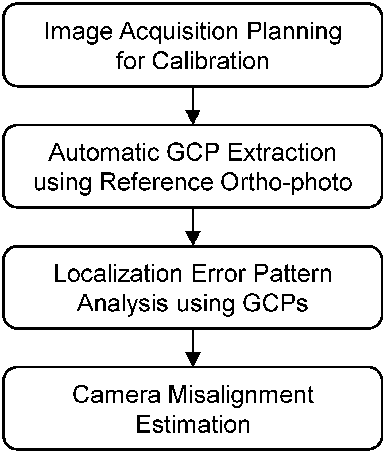
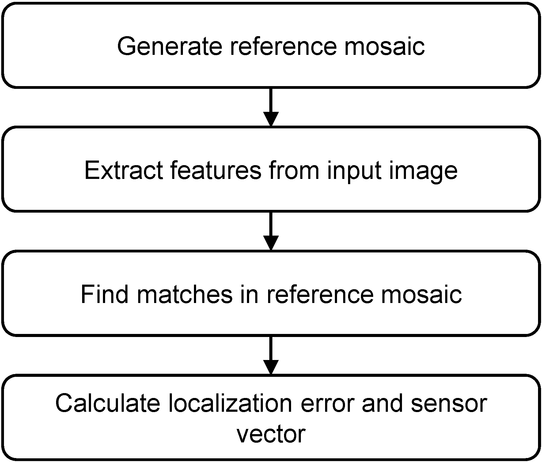
Conceptually, the estimation process of camera misalignment consists of four major steps. The first step is planning the satellite’s imaging operation to acquire image data for the camera misalignment estimation. Extracting GCPs from the images is the next step. Analyzing the error pattern of GCPs and confirming the existence of misalignment are followed. The last step is to estimate the camera misalignment using the GCPs and spacecraft ancillary, which contains spacecraft position and attitude data. Figure 1 shows the conceptual process of the camera misalignment estimation.

Figure 1. Conceptual process of camera misalignment estimation.

Figure 1. Conceptual process of camera misalignment estimation.

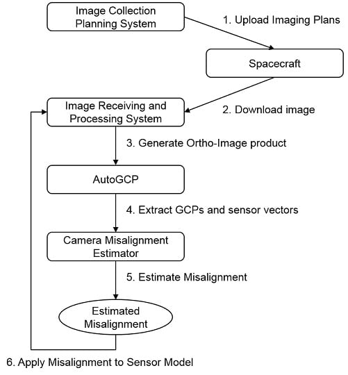
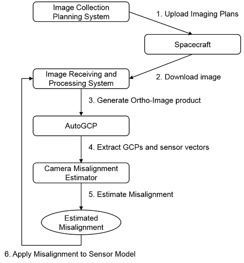
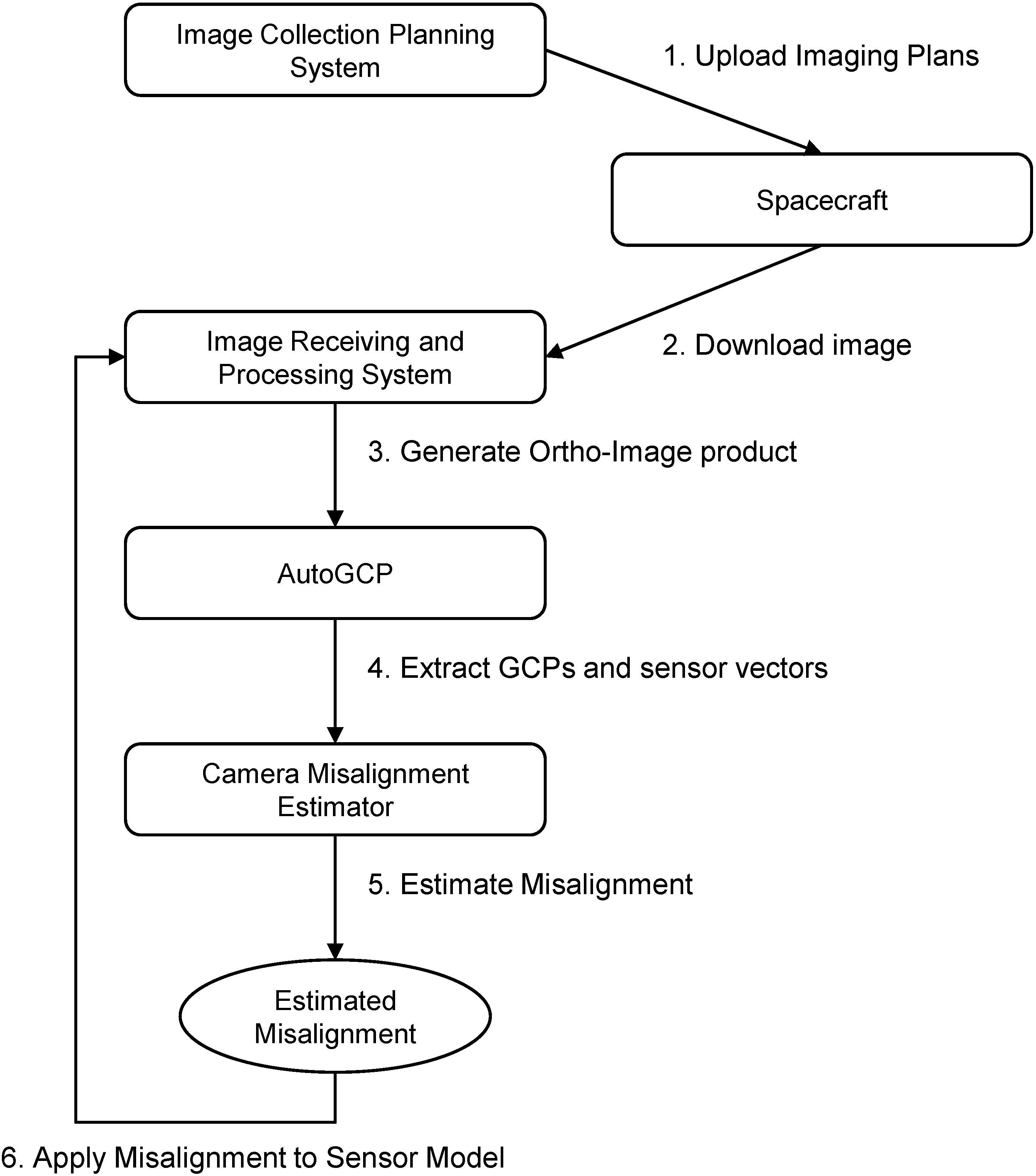
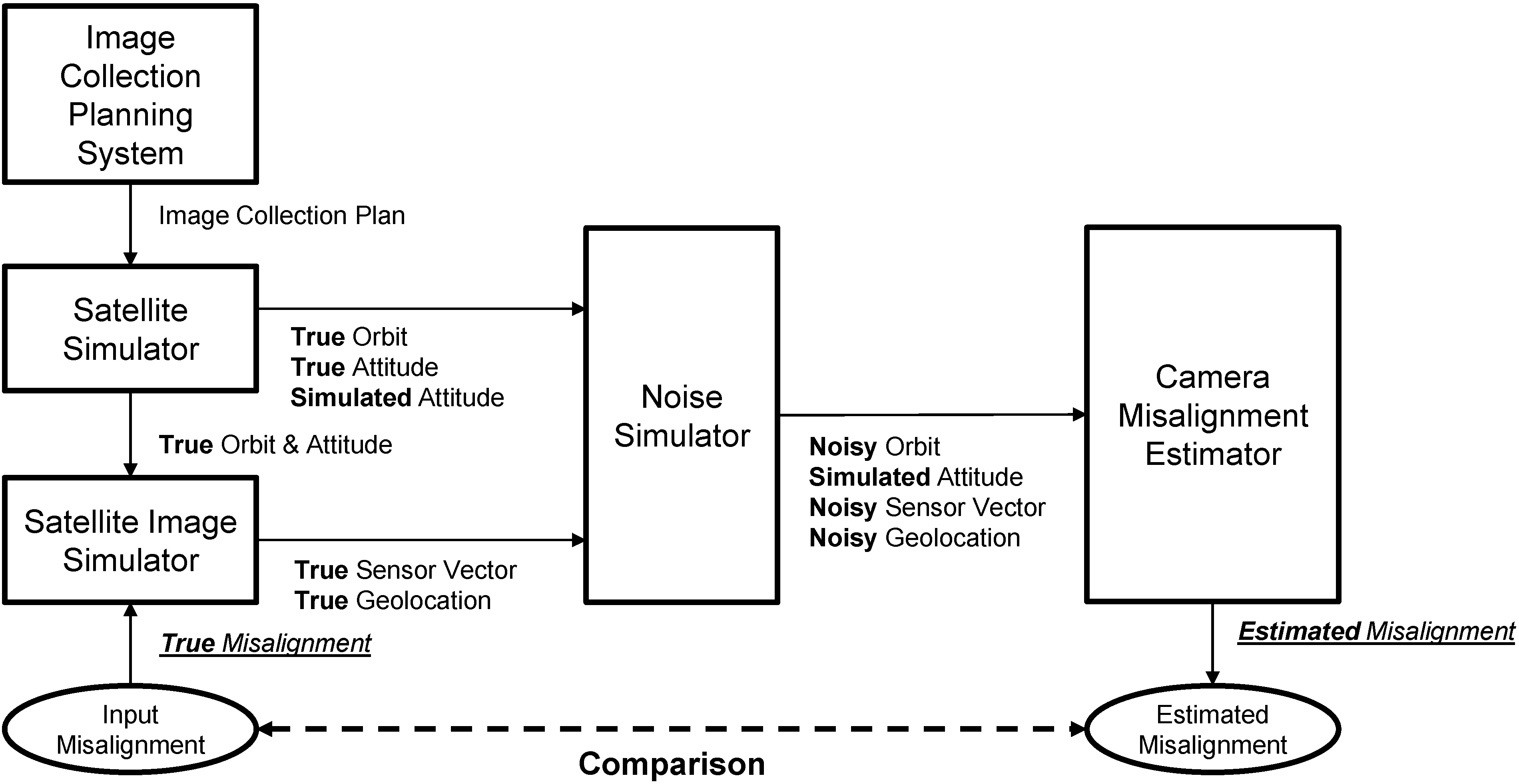
Whereas the simple four steps are provided from a conceptual view, the structural view of camera misalignment estimation involves a couple of additional steps as illustrated in Figure 2.

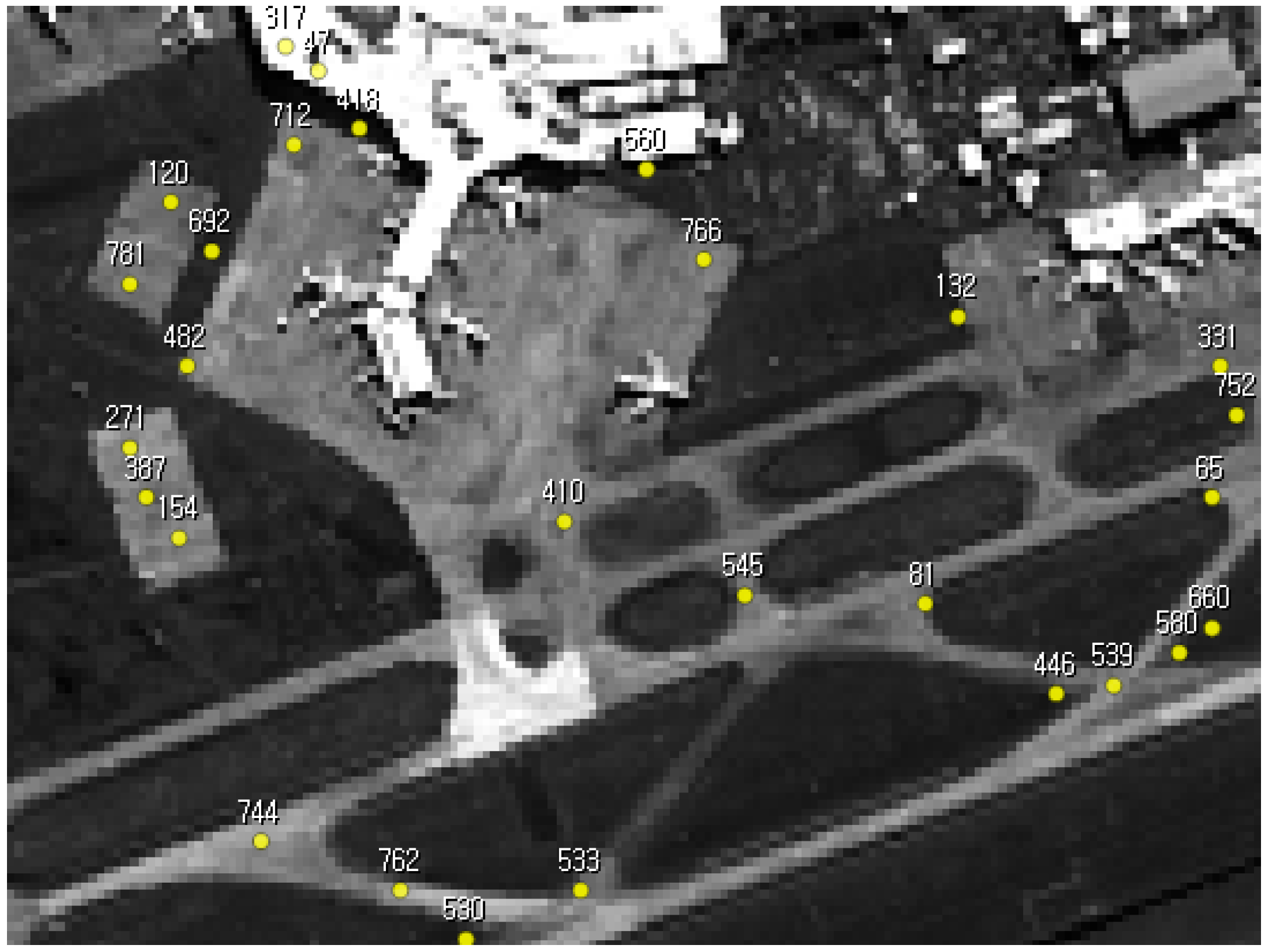
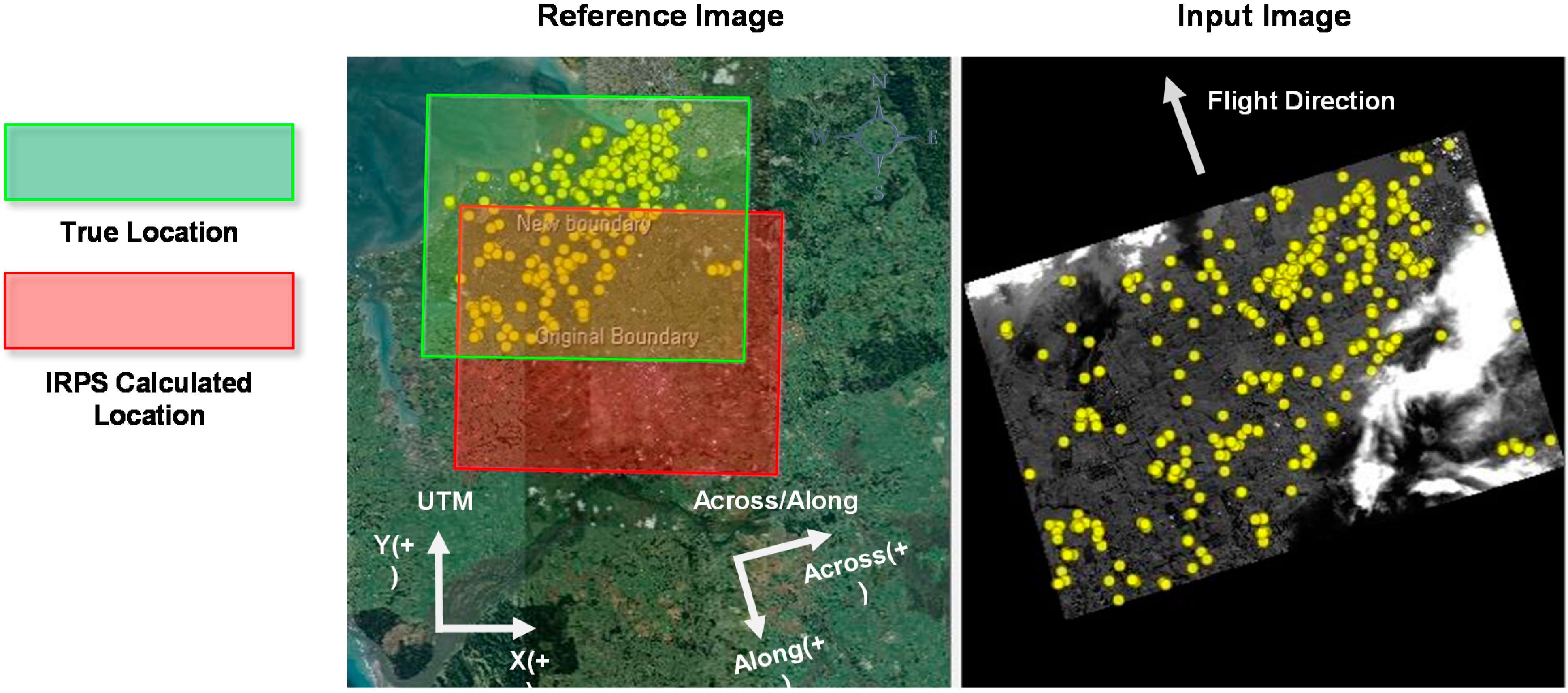
After planning imaging scenarios for calibration, the image collection planning system (ICPS) uploads the plans to the spacecraft (1). After the spacecraft takes images, the images are downloaded to the ground station from the spacecraft (2); thereafter, the image receiving and processing system (IRPS) generates ortho-image products, which consist of geometrically corrected images and spacecraft ancillary data (3). AutoGCP software correlates the images with a reference ortho-photo database and generates GCPs and sensor vectors (4). Camera Misalignment Estimator estimates the camera misalignment by using the results of AutoGCP and spacecraft ancillary data (5). The estimated camera misalignment is then set to IRPS in order to adjust the sensor model (6).

It is recommended to iterate the process (3)–(6) at least a couple of times, because large camera misalignment can make the IRPS use a wrong location for the DEM for geometric correction, which influences the accuracy of the calculated geo-location. Therefore, the camera misalignment needs to be re-estimated after applying the misalignment estimate. The iteration may stop when the change of misalignment estimate is less than the desired accuracy.

Figure 2. Structural process of camera misalignment estimation.

Figure 2. Structural process of camera misalignment estimation.

2.2. Background: Deimos-2

The proposed framework was applied to Deimos-2 which is a high-resolution earth observation satellite equipped with push-broom type CCD sensors providing 1.0 m resolution panchromatic band (PAN) and 4.0 m resolution multispectral band images (blue, green, red, and near-infrared) with 12 km swath width. Since the estimation is done using attitude measurement and image GCPs, it is important to understand the target system’s camera geometry, attitude determination mechanism, and the definitions of attitude and camera frames.

2.2.1. Attitude Sensors

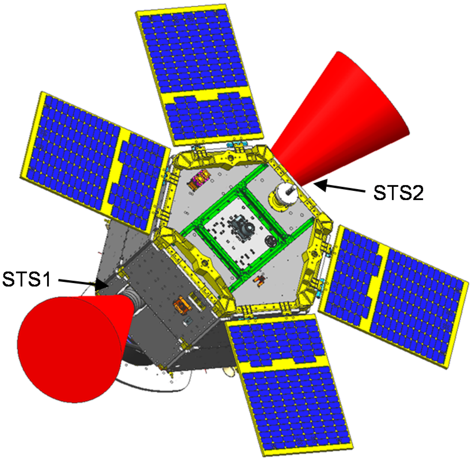
Deimos-2 has two star-trackers for absolute attitude sensing, as well as four gyroscopes for relative attitude sensing. Figure 3 illustrates the exterior configuration of Deimos-2. The red cones are the field-of-view of star-trackers. The gyroscopes are internally equipped. Because the star-trackers are embedded at the opposite side to each other, one of or both star-trackers are selected for the absolute attitude sensing depending on the position and attitude of the satellite during imaging. The electro-optical camera, which is the main payload of Deimos-2, is at the opposite side of the solar panels.

Figure 3. Mounting configuration of Deimos-2 star trackers.

Figure 3. Mounting configuration of Deimos-2 star trackers.

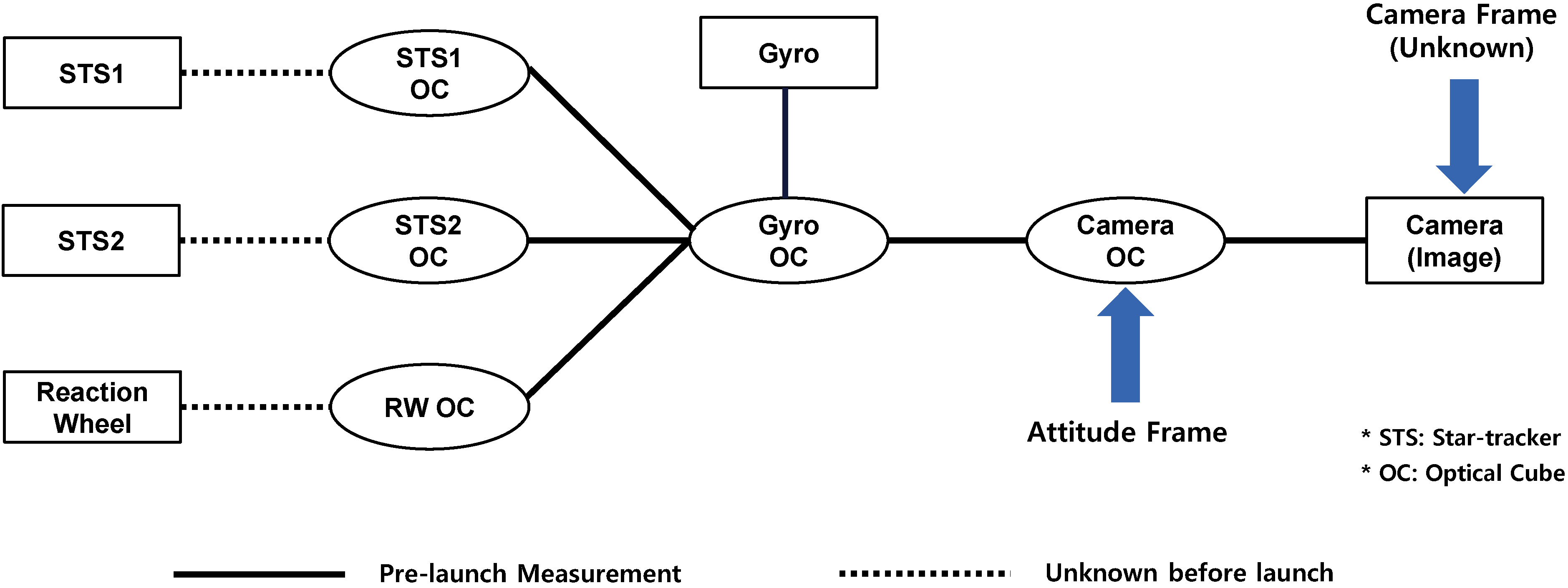
Figure 4 shows the relationship of sensors/actuators and the optical cubes. The sensors and actuators for attitude determination and control are aligned by using optical cubes (OC) before launch. Optical cubes are used as a reference object for precision alignment in satellite manufacturing. The components that need inter-alignment such as imaging sensors and attitude sensors have their own optical cubes that are carefully aligned with them. The alignment between optical cubes are precisely measured using theodolites. Although pre-launch measurement was done for some components, the alignment needs to be calibrated after launch due to launch shock, outgassing, zero-gravity, thermal effect, etc. The alignment between the star-trackers and their optical cubes were unknown due to difficulty in ground measurement. The measurement of angles between optical cubes is used to build a rotation matrix that converts a vector of one component’s frame to the vector of another component’s frame. For Deimos-2, the attitude data in spacecraft ancillary which IRPS uses is based on Camera OC frame, which is also known as Attitude frame. The attitude measured using star-trackers is converted to Camera OC frame. The camera misalignment estimation that described in this paper estimates the discrepancy between this attitude and the GCPs acquired from the image that is in the unknown Camera frame. Hence, the combined error between the attitude sensor and the camera is estimated.

Figure 4. Alignment map of attitude sensors and camera.

Figure 4. Alignment map of attitude sensors and camera.

The alignments between sensors/actuators and optical cubes are calibrated after launch by space-level calibration. Space-level calibration is a series of operations performed during early operation phase, which consists of attitude calibration maneuver and stellar imaging for alignment calibration.

2.2.2. Camera Geometry

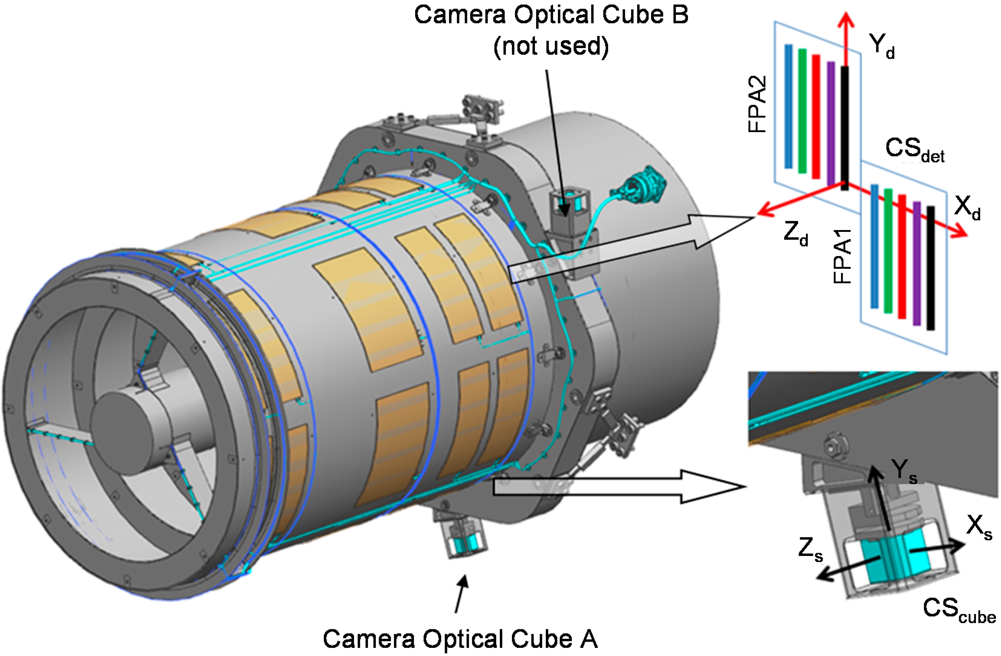
Figure 5 shows the sensor geometry of Deimos-2 camera system. The alignment of the camera system is aligned with the spacecraft body using the Camera OC (Optical Cube) A. The alignment between the coordinates system of Camera OC A, CS_cube, and the coordinates system of the camera focal plane, CS_det, is measured before launch. Two focal plane assemblies (FPA1, FPA2) are aligned to have ground footprints perpendicular to the flight direction with a small overlap (100 panchromatic pixels). The linear TDI CCD arrays are positioned with the order of panchromatic, blue, green, red, and near-infrared in along-track direction. The 6115-th pixel in panchromatic FPA2 is the reference detector that defines the origin and Z-axis direction of the camera frame, which is CS_det.

Figure 5. Geometry of Deimos-2 camera.

Figure 5. Geometry of Deimos-2 camera.

2.2.3. Reference Frames

In this section, the reference frames (a.k.a. reference coordinate systems) used in this paper are defined in detail. For well-known frames such as Earth-centered inertial (ECI) and earth-centered earth-fixed (ECEF), J2000 and WGS-84 are used respectively. The definitions of the Deimos-2 attitude frame and camera frame are presented in Table 1.

The attitude frame is the basis of attitude information in spacecraft ancillary data. It is defined by Camera OC in Deimos-2 as shown in Figure 4. Note that the definitions of the camera system and attitude reference system in Table 1 are the same for Deimos-2. Other spacecrafts may employ different definitions, requiring a rotation matrix to calculate the camera frame from a spacecraft attitude. It is represented by the rotation matrix ${\text{R}}_{\text{Cam}}^{\text{Att}}$ and its inverse ${\text{R}}_{Att}^{Cam}$ in this paper. They are identity matrices for Deimos-2.

Table 1. Definitions of Attitude Frame and Camera Frame.

	Attitude Frame	Camera Frame
Origin	Spacecraft center of mass	Reference detector
Z	Boresight vector of the reference detector	Boresight vector of the reference detector
Y	Longitudinal direction of linear CCD (along with Geometric Y axis direction)	Longitudinal direction of linear CCD (along with Geometric Y axis direction)
X	Y × Z (right hand rule)	Y × Z (right hand rule)

Table 1. Definitions of Attitude Frame and Camera Frame.

	Attitude Frame	Camera Frame
Origin	Spacecraft center of mass	Reference detector
Z	Boresight vector of the reference detector	Boresight vector of the reference detector
Y	Longitudinal direction of linear CCD (along with Geometric Y axis direction)	Longitudinal direction of linear CCD (along with Geometric Y axis direction)
X	Y × Z (right hand rule)	Y × Z (right hand rule)

The camera frame is used by sensor vectors, which point at the corresponding detector cells. IRPS and AutoGCP use sensor vectors to convert image coordinates to geographic coordinates and vice versa.

2.3. Image Planning

The first step is planning imaging scenarios for camera misalignment estimation. It is important to cover all of the possible imaging scenarios that can occur during normal operation. The criteria that needs to be considered for a reliable and accurate estimation are as below.

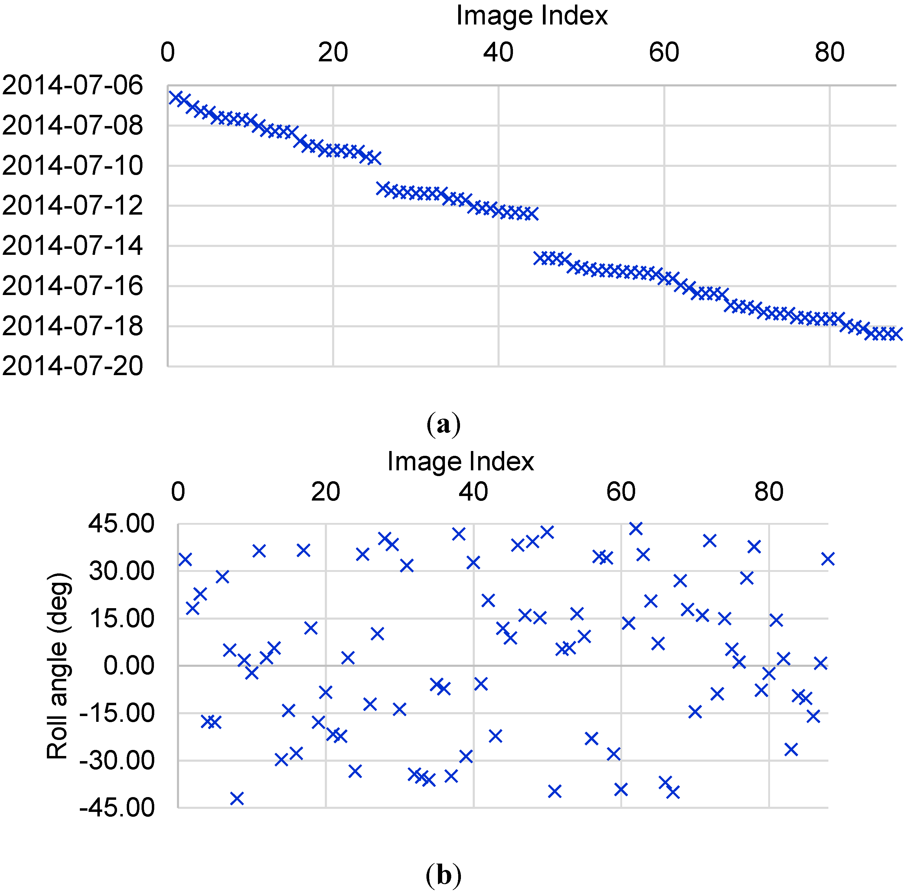
• Tilt angle coverage
• Attitude sensor coverage
• Global coverage
• Terrain variation
• Visual distinctiveness

Tilt angle coverage: The image dataset for camera misalignment estimation needs to use various tilt angles that the spacecraft provides to get a reliable estimation result.

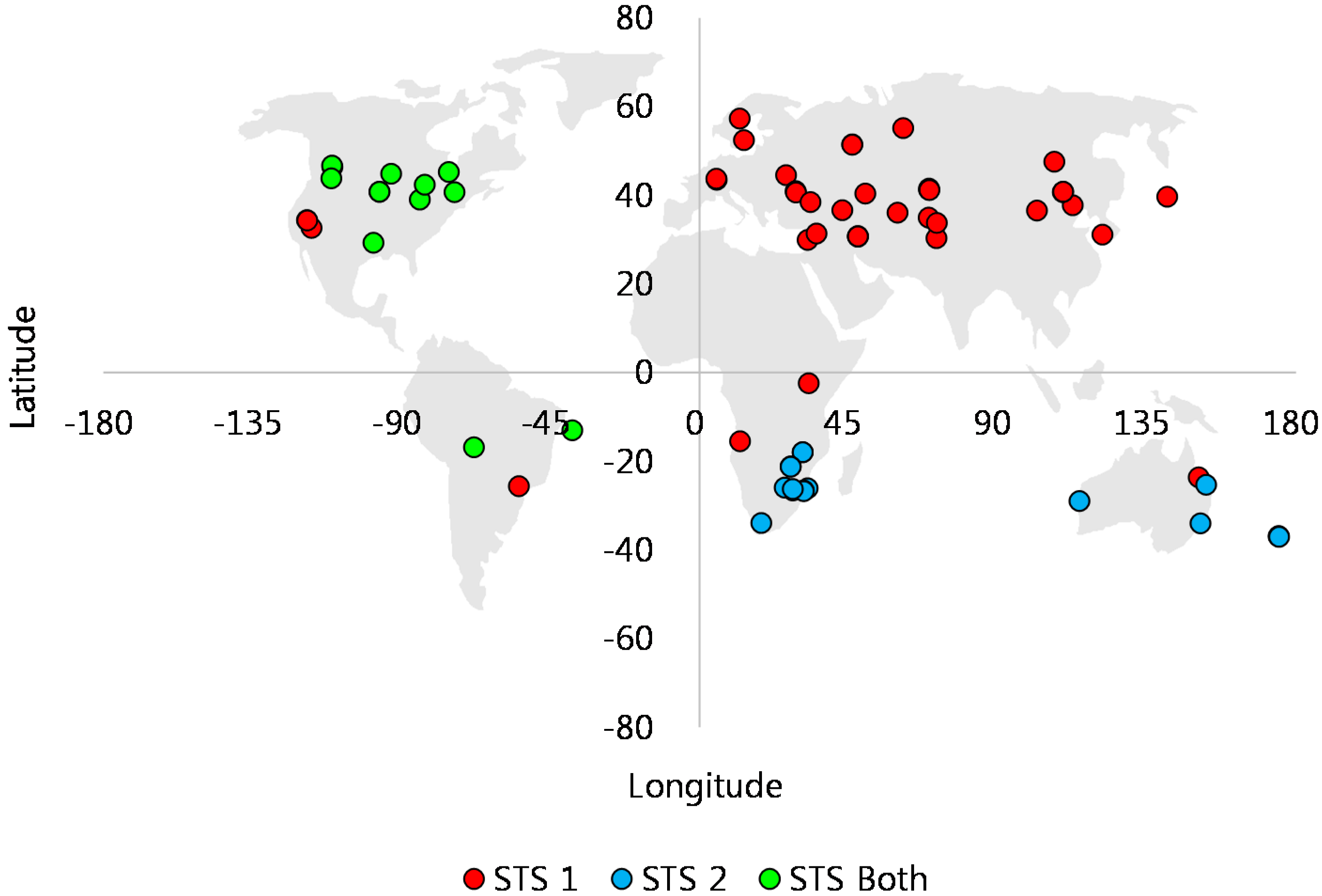
Attitude sensor coverage: If the spacecraft has multiple attitude sensors, those sensors are likely to have different misalignment toward the attitude frame. Since the attitude misalignment also introduces localization error like the camera misalignment, the estimation of the camera misalignment is influenced by the misalignment of attitude sensors. Therefore, the camera misalignment needs to be estimated separately for each sensor group. Deimos-2 is equipped with two star-trackers, and one or both of them are selected depending on the position and attitude of the spacecraft at the time of imaging.

Global coverage: Ground targets needs to be distributed all over the world covering all longitude and latitude ranges. It is not only beneficial for obtaining reliable results, but it can also show a possible relationship between the localization error and the location of a target.

Terrain variation: For the characteristics of ground targets, flat terrain is preferred in order to avoid possible discrepancy of digital elevation model (DEM) and real terrain.

Visual distinctiveness: Area with many visual features are also preferred. However, downtown areas with sky-scrappers are not recommended as tall buildings may add additional localization error, especially at a high tilt angle.

2.4. Automated GCP Extraction

The process of the camera misalignment estimation requires the comparison of the calculated localization with the true localization for GCPs in the images. However, it is exhausting work to obtain a large number of GCPs from many images manually.

Automated GCP extraction software generates GCPs from a geo-coded ortho-image and the corresponding reference dataset and measures the localization error between them. The reference dataset could be geo-coded ortho-rectified images such as LandSat-5 imagery or publicly available satellite imagery service such as Google Maps™. Figure 6 illustrates the process of the automated GCP extraction.

Figure 6. Process of automatic GCP extraction.

Figure 6. Process of automatic GCP extraction.

The first step is to generate a reference image mosaic. The search region is determined by the geo-location information embedded in the input image. The input image before the camera misalignment correction can be located at a different place from the actual location. In order to cover all possible areas, the search region is set to an expansion of the original input image boundary by a certain ratio. A reference mosaic image for the search region is then generated from the reference image database.

In order to extract image features from the input image, GFTT (Good Feature To Track) feature detector in OpenCV, which is based on Shi and Tomoshi’s method [23], is used for corner detection. To ensure features are distributed all over the image, the minimum distance between features $d$ is enforced as follows,

$$d=\text{α}{\left(\frac{w\cdot h}{N}\right)}^{0.5}$$

(1)

where $N$ is the maximum number of features to be extracted, $w$ and $h$ are image width and height, $\text{α}$ is a flexibility parameter which is decided empirically to be 0.5.

The corresponding features in the reference mosaic are found by using a Template Matching method. A comparison region, which is as large as the input image boundary, is chosen from the search region. The features in the input image are searched from the comparison region. Finding the related features within a comparison region reduces the chance of false matches, in comparison to searching in the whole search region. Normalized cross-correlation metric is used as a similarity measure. Each feature of the input image is searched within the comparison region for the similar feature by template matching. The size of search window for template matching is large (e.g., 150 pixels), and the search offset for matching is (0, 0) at the beginning. They are optimized as the number of matches increases as follows,

$$\begin{gathered} e_i=u_i-v_i, i=1\dots N \\ p=median(e_i) \\ s=\beta \times stdev(e_i-p) \end{gathered}$$

(2)

where the offset error $e_i$ is the difference between the input image feature $v_i$ and the comparison region feature $u_i$. $N$ is the total number of features. The search offset $p$ is the median of offset errors of matches, eliminating outliers. The search window size $s$ is the standard deviation of median-centered offset times margin factor $\text{β}$. In this paper, 3.0 is used for $\text{β}$.

When the searching for matches is completed, a homography matrix is estimated by using RANSAC method, so that the outliers are filtered out and inliers are reprojected. The comparison region is moved to another location within the search region to find better matches. The simulated annealing method was used to choose the next location of the comparison region. It chooses a random location at first, but it reduces its randomness as the iteration goes on, so that it can search near the last successful region. The iteration stops when the number of matches is the same as that of the last iteration. Figure 7 shows an example of feature matching results.

Figure 7. Correspondences between reference ortho-photo and input ortho-image.

Figure 7. Correspondences between reference ortho-photo and input ortho-image.

Since the reference mosaic image is geo-referenced, the input image coordinates and the corresponding true geographic locations for each matched pair can be extracted, as well as the localization error of each pair. In order to use GCPs for camera misalignment estimation, the image coordinates need to be converted to sensor vectors.

A sensor vector is a unit direction vector in the camera frame pointing to the detector cell that corresponds with the image coordinates. In order to get a sensor vector from the image coordinates of the input image, the physical camera model that generated the input image performs the inverse mapping.

For each GCP, its IRPS-calculated geo-location, which differs from the true geo-location, could be re-projected onto the focal plane using the spacecraft position and attitude. Since, it is a push-broom sensor, it is not straightforward because the spacecraft takes an image over a certain period. The position and attitude of the moment that the GCP was imaged are necessary for re-projection, however, the time of that moment is unknown. In order to find the time t, an iterative method is used. Firstly, the center time of the imaging duration is used as the initial value of t, and the position and attitude of it is used for re-projection. The re-projected point on the focal plane shall not fall on the sensor because the position and attitude of the wrong time were used. The flight-direction distance between the sensor and the re-projected point is converted to time, and update t with it to move the point to the sensor. The ground point is re-projected with the position and attitude of the new time t. It requires a few iterations until the re-projected point falls on a detector cell. When the point is pointing a detector of the sensor, the vector pointing the re-projected point from the origin of the camera frame is the sensor vector of the GCP. Leprince et al. [24] presented a similar inverse mapping algorithm, however, our approach provide less time-complexity as it uses only one inverse mapping per iteration while theirs require two forward mappings per iteration to use the gradient minimization method.

The results of this process (i.e., GCP geo-location, sensor vector, time t, localization error of GCPs) are stored for camera misalignment estimation.

Figure 8 and Figure 9 show the output of AutoGCP software, which performs the work described in this section. The localization error $\text{ε}$ of each GCP is calculated as follows,

$$\text{ε}=x_{irps}-x_{ref}$$

(3)

where $x_{irps}$ is the UTM coordinate calculated by IRPS using the spacecraft ancillary, and $x_{ref}$ is the UTM coordinate of the reference image.

Figure 8. Measured localization error.

Figure 8. Measured localization error.

An important coordinates system for localization error analysis is spacecraft across/along-track coordinates system, which is defined by increasing column/line number direction. The analysis of localization errors in across/along-track direction makes it possible to analyze the errors in comparison with other imaging parameters such as tilt angles and target locations. Since the reference image and input ortho-image are generally in UTM projection, the localization error in UTM projection could be easily calculated. The conversion to spacecraft across/along-track direction from UTM X/Y direction could be done using the flight direction vector. Figure 10 shows the comparison of UTM X/Y direction and spacecraft across/along-track direction. Note that the along-track (+) direction is defined as the opposite of the flight direction in this paper, even though it is customary to set them to the same direction.

Figure 9. Extracted GCPs.

Figure 9. Extracted GCPs.

Figure 10. Comparison of UTM and across/long-track direction.

Figure 10. Comparison of UTM and across/long-track direction.

2.5. Error Pattern Analysis

Analyzing the pattern of localization error helps to find the existence of camera misalignment as well as other issues such as time drift. The estimation and correction of camera misalignment is meaningful when there is an obvious pattern of camera misalignment. It also is useful to know what type and amount of camera misalignment are there before estimation.

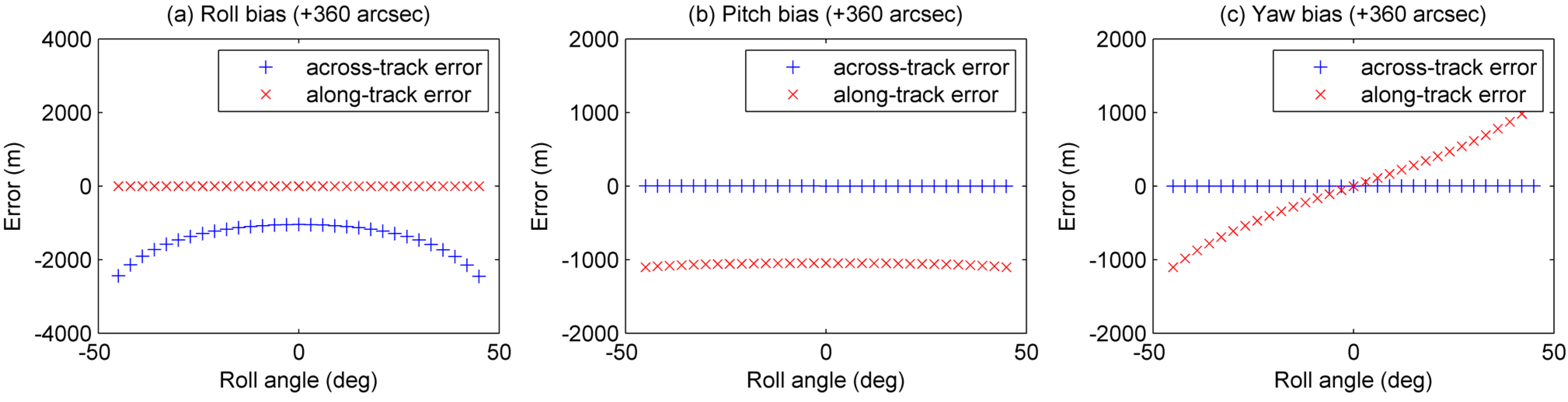
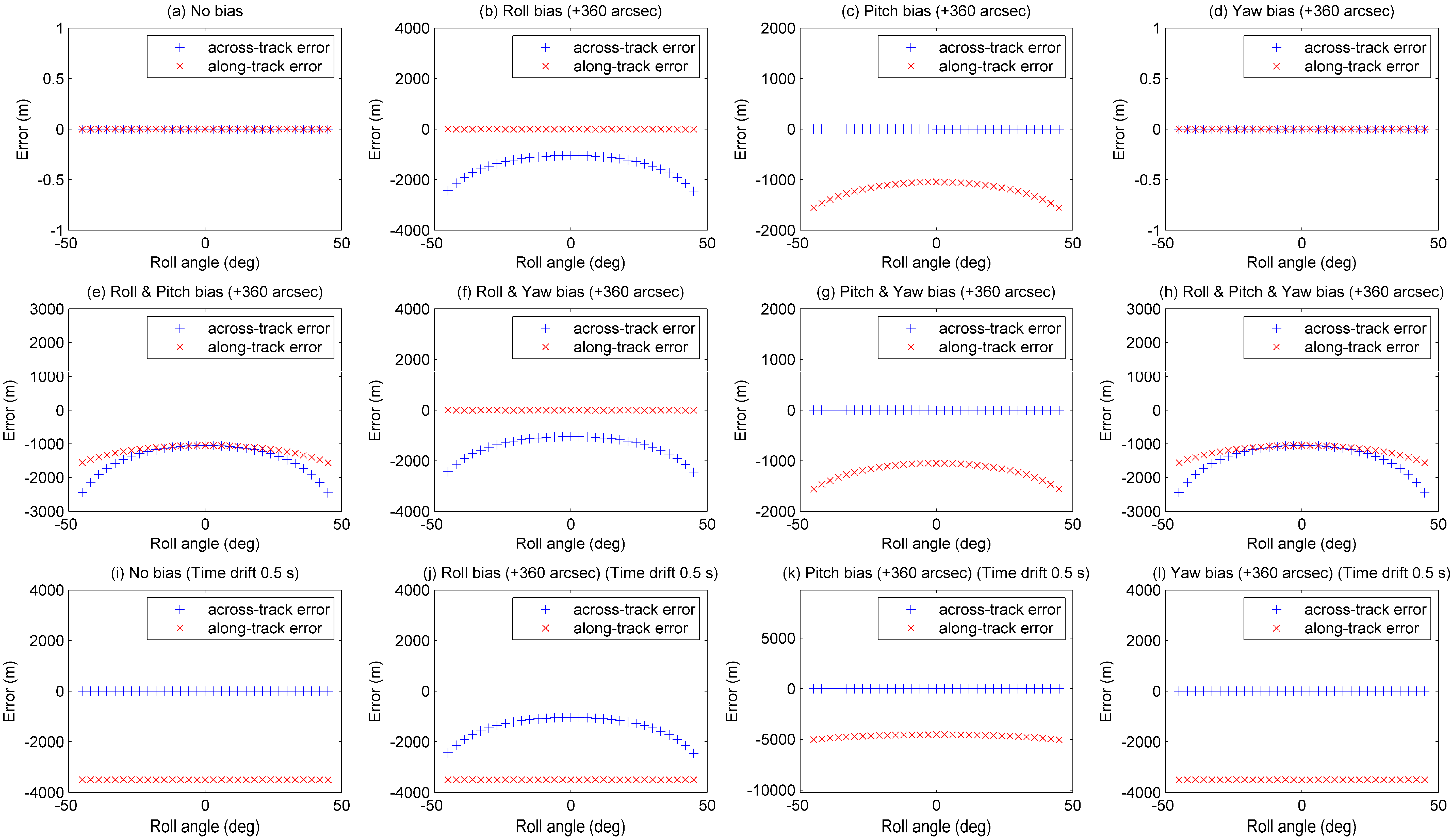
If a camera misalignment exists, a correlation between the tilt angle and localization error can be observed. Figure 11 shows the plots of localization error on various camera misalignments. Note that changing the sign of the misalignment will create localization errors of the opposite sign.

Figure 11. Localization errors by camera misalignment: (a) No bias, (b) Roll bias (+360 arcsec), (c) Pitch bias (+360 arcsec), (d) Yaw bias (+360 arcsec), (e) Roll & Pitch bias (+360 arcsec), (f) Roll & Yaw bias (+360 arcsec), (g) Pitch & Yaw bias (+360 arcsec), (h) Roll & Pitch & Yaw bias (+360 arcsec), (i) No bias (Time drift 0.5 s),(j) Roll bias (+360 arcsec) (Time drift 0.5 s), (k) Pitch bias (+360 arcsec) (Time drift 0.5 s), (l) Yaw bias (+360 arcsec) (Time drift 0.5 s).

Figure 11. Localization errors by camera misalignment: (a) No bias, (b) Roll bias (+360 arcsec), (c) Pitch bias (+360 arcsec), (d) Yaw bias (+360 arcsec), (e) Roll & Pitch bias (+360 arcsec), (f) Roll & Yaw bias (+360 arcsec), (g) Pitch & Yaw bias (+360 arcsec), (h) Roll & Pitch & Yaw bias (+360 arcsec), (i) No bias (Time drift 0.5 s),(j) Roll bias (+360 arcsec) (Time drift 0.5 s), (k) Pitch bias (+360 arcsec) (Time drift 0.5 s), (l) Yaw bias (+360 arcsec) (Time drift 0.5 s).

Whilst roll and pitch biases display distinct patterns, yaw bias does not show a strong pattern in Figure 11d. It is because the yaw angle of the camera misalignment has small effect in localization error. The localization error $\text{ε}$ that is generated by the yaw error at the end of the CCD array can be calculated as follows,

$$\text{ε}=\frac{1}{2}{\text{ϑ}}_{z}LD$$

(4)

where ${\text{ϑ}}_z$ is the yaw-bias in radian, $L$ is the CCD array length, and D is the pixel GSD. Because of its relatively small error even with high tilt angles, it is difficult to estimate the yaw bias.

Sometimes, the ancillary data, which contains position and attitude, can have time offset or drift error. If time offset exists, along-track error has an offset as depicted in Figure 11i–l. In this case, it is difficult to relate to one of the biases in Figure 11b–h. In case of time drift, it should be corrected before estimating the camera misalignment. Since there are many sources that can cause time drift phenomena, the estimation of time drift is not discussed in this paper.

Another major source of localization error that can be confused with camera misalignment is attitude misalignment. The misalignment in the attitude frame affects the control and determination of the spacecraft attitude, resulting localization errors. Figure 12 shows the plots of localization error on various attitude misalignments. While the localization error induced by the yaw bias in the camera frame is hardly observable due to narrow field of view as shown in Figure 11d, it is clearly visible in Figure 12c that the yaw bias in the attitude frame generates large error as the tilt-angle increases.

Figure 12. Localization errors by attitude misalignment: (a) Roll bias (+360 arcsec), (b) Pitch bias (+360 arcsec), (c) Yaw bias (+360 arcsec).

Figure 12. Localization errors by attitude misalignment: (a) Roll bias (+360 arcsec), (b) Pitch bias (+360 arcsec), (c) Yaw bias (+360 arcsec).

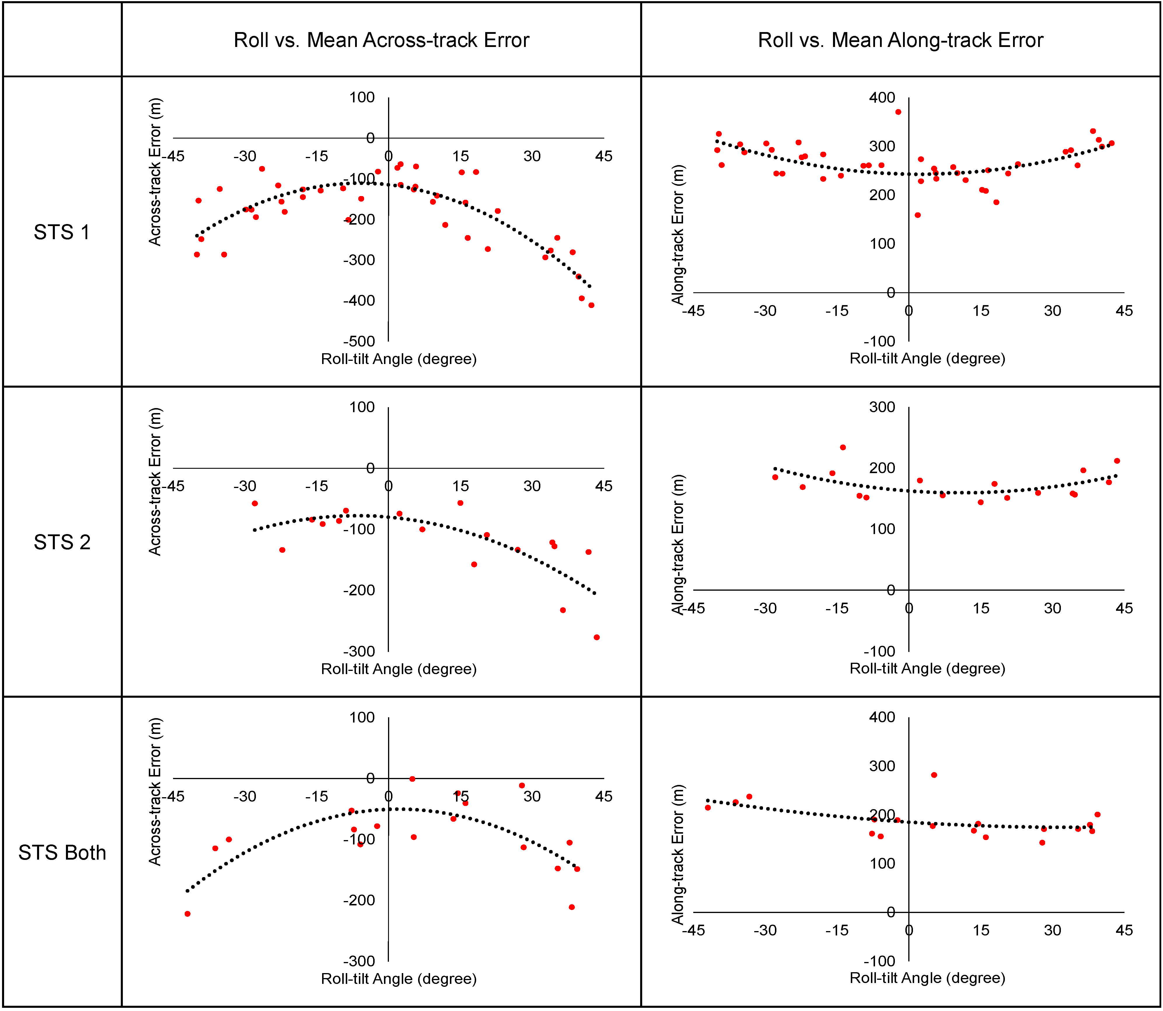
There are many other error sources of localization error such as star-trackers, gyroscopes, focal plane assemblies, sensor arrays, or somewhere between them. Only the sum of all misalignments from the attitude sensors to the camera image plane could be observed from image GCPs and attitude data. It is important to categorize datasets that can have different misalignment for effective analysis. In Section 3.2, Since Deimos-2 has two star-trackers and they are selected depending on the spacecraft attitude, its localization errors were analyzed for star-tracker selections.

In case that localization errors and tilt angles cannot be correlated, the cause of error may not be camera misalignment. They can be sensor malfunctioning, on-board software errors, or inconsistency of ancillary data. It is also recommended to analyze the relationship between the localization errors and target locations (longitude, latitude). Depending on the thermo-elastic characteristics of the spacecraft or the orbit design, the location of the target can affect the localization error.

2.6. Camera Misalignment Estimation

This section describes a mathematical model for camera misalignment estimation. The model describes the relationship between spacecraft position, attitude, sensor vector, and GCP. The key idea of the proposed estimation model is to calculate the boresight misalignment, which is the angular error between the camera frame and the true camera frame, using GCPs and spacecraft positions/attitudes. In order to simplify the problem, the origins of the attitude frame and the camera frame are assumed to be the same.

Assuming that there is no camera misalignment, the geometrical relationship can be modelled as follows:

$$p_S^{Cam}=R_{Att}^{Cam}{R_t}_{ECI}^{Att}{p}_G^{ECI}$$

(5)

where,

$$p_S^{Cam}=\left[\frac{T_S^{Cam}}{\Vert T_S^{Cam}\Vert }\right],T_S^{Cam}=\left[\begin{array}{c}x\\ y\\ -f\end{array}\right],p_G^{ECI}=\left[\frac{T_G^{ECI}-{T_t}_S^{ECI}}{\Vert T_G^{ECI}-{T_t}_S^{ECI}\Vert }\right]$$

(6)

$p_S^{Cam}$ is a sensor vector, which is a unit vector of the vector $T_S^{Cam}$, which points the detector pixel on the focal plane at which a GCP is located. $R_{Att}^{Cam}$ and ${R_t}_{ECI}^{Att}$ are rotation matrices from attitude frame to camera frame, and from ECI frame to attitude frame, respectively, at time $t$. $p_G^{ECI}$ is an object vector in ECI frame pointing the GCP from the spacecraft. $T_G^{ECI}$ is a position vector of ground object G in ECI frame. ${T_t}_S^{ECI}$ is a position vector of spacecraft in ECI frame at time $t$. Since the geo-locations of GCPs are generally in LLH or ECEF, it is important to convert the coordinate system to ECI to get $p_G^{ECI}$.

In order to take account for the camera misalignment, a bias-correction matrix $R_{Cam}^{TrueCam}$ is added:

$$p_S^{TrueCam}=R_{Cam}^{TrueCam}{R}_{Att}^{Cam}{R_t}_{ECI}^{Att}{p}_G^{ECI}$$

(7)

In practice, the amount of misalignment is less than one degree (i.e., 3600 arcsec). Therefore, an approximation for infinitesimal rotations can be used to solve Equation (7). Supposed that the misalignment is an Euler-angle rotation ${\text{ϑ}}_{TrueCam}$,

$${\text{ϑ}}_{TrueCam}=\left[\begin{array}{c}{\text{ϑ}}_x\\ {\text{ϑ}}_y\\ {\text{ϑ}}_z\end{array}\right]$$

(8)

where ${\text{ϑ}}_{\mathrm{x}}$, ${\text{ϑ}}_{\mathrm{y}}$, ${\text{ϑ}}_{\mathrm{z}}$ are roll, pitch, yaw bias respectively, it can be approximated as follows [25,26]:

$$R_{Cam}^{TrueCam}\approx I+\left[{\text{ϑ}}_{TrueCam}\times \right]$$

(9)

$$\left[{\text{ϑ}}_{TrueCam}\times \right]=\left[\begin{array}{ccc}0& -{\text{ϑ}}_z& {\text{ϑ}}_y\\ {\text{ϑ}}_z& 0& -{\text{ϑ}}_x\\ -{\text{ϑ}}_y& {\text{ϑ}}_x& 0\end{array}\right]$$

(10)

The error of the small angle approximation of sine and cosine function is less than 1% for angles smaller than 14 degrees (≈50,000 arcsec).

In consequence, the equation for a sensor vector and a unit object vector in the Equation (7) can be expanded as below.

$$p_S^{TrueCam}\approx \left(I+\left[{\text{ϑ}}_{TrueCam}\times \right]\right)R_{ECI}^{Cam}{p}_G^{ECI}$$

(11)

$$=R_{ECI}^{Cam}{p}_G^{ECI}+\left[{\text{ϑ}}_{TrueCam}\times \right]R_{ECI}^{Cam}{p}_G^{ECI}$$

(12)

$$=R_{ECI}^{Cam}{p}_G^{ECI}-\left[R_{ECI}^{Cam}{p}_G^{ECI}\times \right]{\text{ϑ}}_{TrueCam}$$

(13)

Equation (13) can be rewritten as follows, which forms a normal equation for linear least squares (Ax = b):

$$\left[R_{ECI}^{Cam}{p}_G^{ECI}\times \right]{\vartheta }_{TrueCam}=R_{ECI}^{Cam}{p}_G^{ECI}-p_S^{TrueCam}(\text{Ax}=\text{b})$$

(14)

In addition to the Equation (14), a weight matrix $W$ is introduced to adjust weight of each observation and to force pre-defined bias to certain axes as below:

$$WAx=Wb$$

(15)

where the weight matrix $W$ is defined as:

$$\begin{gathered} W_{\left(3\left(N+1\right)\times 3\left(N+1\right)\right)}=\left[\begin{array}{cccc}{W}_1& & & \\ & \ddots & & \\ & & W_N& \\ & & & r\end{array}\right], \\ {W}_{i=1\dots N}=diag\left(\begin{array}{ccc}\frac{1}{{\sigma }_i^2}& \frac{1}{{\sigma }_i^2}& \frac{1}{{\sigma }_i^2}\end{array}\right), r_{(3\times 3)} =\left[\begin{array}{ccc}\frac{1}{r_x^2}& & \\ & \frac{1}{r_y^2}& \\ & & \frac{1}{r_z^2}\end{array}\right] \end{gathered}$$

(16)

Other elements (i.e., $A$, $b$, $x$) in the Equation (15) are also extended as follows,

$$\begin{gathered} x={\text{ϑ}}_{TrueCam}, A=\left[\begin{array}{c}\begin{array}{c}{H}_i\end{array}\\ I_{\left(3\times 3\right)}\end{array}\right], b=\left[\begin{array}{c}{M}_i\\ V\end{array}\right] \\ {H}_{i=1\dots N}=\left[\begin{array}{c}{R_i}_{ECI}^{Cam}{p_i}_G^{ECI}\times \end{array}\right] \\ {M}_{i=1\dots N}=\left[{R_i}_{ECI}^{Cam}{p_i}_G^{ECI}-{p_i}_S^{TrueCam}\right] \\ V={\left[\begin{array}{ccc}{\text{θ}}_x& {\text{θ}}_y& {\text{θ}}_z\end{array}\right]}^T \end{gathered}$$

(17)

$W_{i=1\dots N}$ sets the weight for each observation in accordance with the accuracy of observation. In case that every observation has the same accuracy, the weight is set to 1.0. However, it can also be set to a certain weight calculated from the accuracy of observation, such as the geo-accuracy of a GCP, sensor vector, and position/attitude knowledge.

$V$ and $r$ could be used to set the bias of some axes to given values. $r$ is a parameter for choosing whether the pre-assigned bias will be enforced or not. Setting the element of $r$ to a very small number (e.g., 10⁻¹°) forces the assigned angle in $V$ to be the bias of the given axis, whereas setting it to a very large number (e.g., 10¹°) means $V$ is ignored. It is useful when the visibility of a certain axis is expected to be very low due to narrow field of view; for instance, the yaw axis of high-resolution push-broom imaging sensors.

Solving Equation (15) gives a least squares solution of ${\vartheta }_{TrueCam}$, which contains estimated camera misalignment angles in radian. In order to compensate the camera misalignment during ortho-image generation, the alignment of camera frame from attitude frame needs to be updated using ${\text{ϑ}}_{TrueCam}$. The new rotation matrix $R{´}_{Att}^{Cam}$ is calculated as follows,

$$R{´}_{Att}^{Cam}=DCM({\text{ϑ}}_{TrueCam})R_{Att}^{Cam}$$

(18)

where $DCM({\text{ϑ}}_{TrueCam})$ is a direction cosine matrix for ${\text{ϑ}}_{TrueCam}$, and $R_{Att}^{Cam}$ is the original rotation matrix. The order of rotations is irrelevant for infinitesimal angles [25,26].

3. Experimental Section

3.1. Simulation

3.1.1. Data

The objectives of simulation tests are to prove the validity of the estimation model and obtain expected accuracy before the application to real image data. The test environment was set up as illustrated in Figure 13. Three additional components were used to simulate an actual spacecraft, compared to Figure 2.

Figure 13. Environment setup for simulation test.

Figure 13. Environment setup for simulation test.

Satellite Simulator simulated the spacecraft system in space environment. It ran the same on-board software emulating all the position/attitude sensors and actuators of Deimos-2. As it complied the design specification of Deimos-2 hardware, it could simulate realistic behavior of a spacecraft on orbit. Image Simulator generated simulated imagery taken by the simulated spacecraft. It also generated sensor vectors and their corresponding geo-locations, which were the output of AutoGCP. Noise Simulator added noise to orbit data, sensor vectors, and geo-locations for realistic simulation.

Table 2 shows the categories of the experiments. The first category is the no noise category, which verifies if the proposed estimation model is capable of estimating camera misalignment in ideal cases. The second category is the noise category, which provides the estimated accuracy for real cases.

Table 2. Image Simulation Setting.

	No Noise			Noise
Number of images	1			Same
Size of image	6000 × 6000			Same
Attitude (deg.)	Roll	Pitch	Yaw	Same
	−4.243	+0.109	0
Number of GCPs per image	270			Same
Spacing between GCPs	350 m			Same
Position Error (Gaussian) (meter)	0 m			Along	Across	Radial
				30	5	5
Attitude Knowledge (3σ) (arcsec)	0			Roll	Pitch	Yaw
				360	360	360
Planimetric GCP Error (Gaussian)	0 m			30 m

Table 2. Image Simulation Setting.

	No Noise			Noise
Number of images	1			Same
Size of image	6000 × 6000			Same
Attitude (deg.)	Roll	Pitch	Yaw	Same
	−4.243	+0.109	0
Number of GCPs per image	270			Same
Spacing between GCPs	350 m			Same
Position Error (Gaussian) (meter)	0 m			Along	Across	Radial
				30	5	5
Attitude Knowledge (3σ) (arcsec)	0			Roll	Pitch	Yaw
				360	360	360
Planimetric GCP Error (Gaussian)	0 m			30 m

Image Simulator is capable of setting alignment biases to simulate camera misalignment. In the experiments, eight cases with different combinations of bias values were tested. Camera misalignment Estimator estimated the bias for each case. The assigned bias values and estimated bias values were compared.

3.1.2. Results

Table 3 shows the results of the no noise category. The error of estimation model was up to 0.054 arcsec for all test cases. As 1 arcsec error corresponds to approximately 3.3 m on ground, it is proven that the model provides sub-meter accuracy for ideal cases. The error of 0.054 arcsec residual under zero noise seems like numerical error, since 0.01 arcsec is 2.61799398e⁻⁷ radian.

Table 3. Misalignment Estimation Results of No Noise Case.

True Bias (arcsec)			Estimated Bias (arcsec)			Error (arcsec)
Roll	Pitch	Yaw	Roll	Pitch	Yaw	Roll	Pitch	Yaw
0	0	0	−0.001	0.006	−0.001	0.001	−0.006	0.001
100	0	0	99.999	0.006	−0.001	0.001	−0.006	0.001
0	100	0	−0.001	100.006	−0.001	0.001	−0.006	0.001
0	0	100	−0.001	0.006	99.999	0.001	−0.006	0.001
100	0	100	99.999	0.054	99.999	0.001	−0.054	0.001
0	100	100	−0.049	100.006	99.999	0.049	−0.006	0.001
100	100	0	99.999	100.006	−0.049	0.001	−0.006	0.049
100	100	100	99.951	100.054	99.951	0.049	−0.054	0.049

Table 3. Misalignment Estimation Results of No Noise Case.

True Bias (arcsec)			Estimated Bias (arcsec)			Error (arcsec)
Roll	Pitch	Yaw	Roll	Pitch	Yaw	Roll	Pitch	Yaw
0	0	0	−0.001	0.006	−0.001	0.001	−0.006	0.001
100	0	0	99.999	0.006	−0.001	0.001	−0.006	0.001
0	100	0	−0.001	100.006	−0.001	0.001	−0.006	0.001
0	0	100	−0.001	0.006	99.999	0.001	−0.006	0.001
100	0	100	99.999	0.054	99.999	0.001	−0.054	0.001
0	100	100	−0.049	100.006	99.999	0.049	−0.006	0.001
100	100	0	99.999	100.006	−0.049	0.001	−0.006	0.049
100	100	100	99.951	100.054	99.951	0.049	−0.054	0.049

Table 4 shows the results of noise category. The errors were around 30 arcsec in roll and pitch biases and around 400 arcsec in yaw bias. In comparison with the sensor accuracy in Table 2, which is 360–432 arcsec, the accuracy of the roll/pitch biases estimation is better than the hardware specification. Given that the attitude error is mainly made of bias and random error, the influence of sensor’s random error in camera misalignment estimation is reduced as more and more data samples are used. However, the yaw bias might still be difficult to estimate accurately, because of the narrow field-of-view of a high-resolution push-broom type sensor. It is not problematic in practice, because it also means that the influence of the yaw bias in the camera frame is relatively low.

Table 4. Misalignment Estimation Results of Noise Case.

True Bias (arcsec)			Estimated Bias (arcsec)			Error (arcsec)
Roll	Pitch	Yaw	Roll	Pitch	Yaw	Roll	Pitch	Yaw
0	0	0	−13.466	13.466	23.545	−23.545	0.659	−0.659
100	0	0	87.880	12.120	29.495	−29.495	−397.391	397.391
0	100	0	−12.542	12.542	129.351	−29.351	259.387	−259.387
0	0	100	−14.160	14.160	20.218	−20.218	132.343	−32.343
100	0	100	86.432	13.568	22.535	−22.535	−140.799	240.799
0	100	100	−14.090	14.090	119.881	−19.881	152.769	−52.769
100	100	0	86.035	13.965	120.356	−20.356	−129.372	129.372
100	100	100	86.431	13.569	123.715	−23.715	190.704	−90.704

Table 4. Misalignment Estimation Results of Noise Case.

True Bias (arcsec)			Estimated Bias (arcsec)			Error (arcsec)
Roll	Pitch	Yaw	Roll	Pitch	Yaw	Roll	Pitch	Yaw
0	0	0	−13.466	13.466	23.545	−23.545	0.659	−0.659
100	0	0	87.880	12.120	29.495	−29.495	−397.391	397.391
0	100	0	−12.542	12.542	129.351	−29.351	259.387	−259.387
0	0	100	−14.160	14.160	20.218	−20.218	132.343	−32.343
100	0	100	86.432	13.568	22.535	−22.535	−140.799	240.799
0	100	100	−14.090	14.090	119.881	−19.881	152.769	−52.769
100	100	0	86.035	13.965	120.356	−20.356	−129.372	129.372
100	100	100	86.431	13.569	123.715	−23.715	190.704	−90.704

In case that the observability of yaw bias is expected to be low, the estimation model could be set to fixate the yaw bias to zero. Table 5 shows there was no noticeable change in the accuracy of roll and pitch bias when the yaw bias was not estimated.

Table 5. Misalignment Estimation Results of Noise Case with Yaw Bias = 0.

True Bias (arcsec)			Estimated Bias (arcsec)			Error (arcsec)
Roll	Pitch	Yaw	Roll	Pitch	Yaw	Roll	Pitch	Yaw
0	0	0	−12.816	12.816	26.028	−26.028	0.000	0.000
100	0	0	86.396	13.604	22.465	−22.465	0.000	0.000
0	100	0	−14.029	14.029	120.620	−20.620	0.000	0.000
0	0	100	−11.551	11.551	32.314	−32.314	0.000	100.000
100	0	100	87.897	12.103	30.500	−30.500	0.000	100.000
0	100	100	−13.540	13.540	123.005	−23.005	0.000	100.000
100	100	0	86.711	13.289	123.092	−23.092	0.000	0.000
100	100	100	87.545	12.455	128.657	−28.657	0.000	100.000

Table 5. Misalignment Estimation Results of Noise Case with Yaw Bias = 0.

True Bias (arcsec)			Estimated Bias (arcsec)			Error (arcsec)
Roll	Pitch	Yaw	Roll	Pitch	Yaw	Roll	Pitch	Yaw
0	0	0	−12.816	12.816	26.028	−26.028	0.000	0.000
100	0	0	86.396	13.604	22.465	−22.465	0.000	0.000
0	100	0	−14.029	14.029	120.620	−20.620	0.000	0.000
0	0	100	−11.551	11.551	32.314	−32.314	0.000	100.000
100	0	100	87.897	12.103	30.500	−30.500	0.000	100.000
0	100	100	−13.540	13.540	123.005	−23.005	0.000	100.000
100	100	0	86.711	13.289	123.092	−23.092	0.000	0.000
100	100	100	87.545	12.455	128.657	−28.657	0.000	100.000

In conclusion, the estimation model is capable of estimating the camera misalignment to sub-meter accuracy under ideal conditions. With realistic simulation data, the estimation accuracy is better than the accuracy of hardware while the yaw estimation does not affect the overall accuracy much.

3.2. Real Image

3.2.1. Data

The estimation framework presented in this paper was applied to Deimos-2 to measure and correct its camera misalignment. It began with listing up candidate targets in the world. Figure 14 shows the distribution of the ground target images used in the experiments.

The targets were focused on populated area containing rich features to obtain enough number of GCPs. The colors of markers (red, green, blue) in the figure represent which star-tracker was selected for on-board attitude determination. Deimos-2 has three star-tracker selection modes (STS 1, STS 2, STS Both) and the figure shows that all selections are included for the test images. Note that the selection is based generally on the location of the ground target as shown in the figure as well as the off-nadir tilt angle.

Figure 14. Ground target distribution of Deimos-2.

Figure 14. Ground target distribution of Deimos-2.

In order to investigate the difference between imaging modes, the images were taken in two imaging modes; Strip and Fast Multi-strip (FMS). In Strip mode, the spacecraft returns to house-keeping mode after imaging, whereas in FMS mode, it performs a maneuver and takes successive images before returning to house-keeping mode. Table 6 shows the number of images collected for camera misalignment estimation.

Table 6. Number of Images Collected For Deimos-2 Calibration.

Imaging Mode	# Images
Strip	37
FMS	51
Total	88

Table 6. Number of Images Collected For Deimos-2 Calibration.

Imaging Mode	# Images
Strip	37
FMS	51
Total	88

Figure 15a shows the distribution of imaging dates. The images were taken over a two-week period. There are gaps at 10 and 14 July 2014 because the spacecraft was dedicated to other priority tasks.

Figure 15b shows the distribution of roll-tilt angles. The images cover all of the roll angle range that Deimos-2 is capable. The pitch angle and yaw angle were all set to zero, since Deimos-2 does not provide pitch and yaw tilt in Strip and FMS imaging mode.

The images were processed to ortho-image products after download. The SRTM DEM which has 90 m accuracy was used for geometric rectification. AutoGCP software extracted GCPs and the corresponding sensor vectors from the ortho-images, and calculated the localization errors. The spatial resolution of reference mosaic for GCP extraction was set to 15 m, which corresponds to the geo-location accuracy of resulting GCPs, accounting for the accuracy of Deimos-2 attitude sensors.

Figure 15. Distribution of (a) imaging dates and (b) roll-tilt angles.

Figure 15. Distribution of (a) imaging dates and (b) roll-tilt angles.

In order to inspect the localization error, the mean ${\text{μ}}_{error}$ and standard deviation ${\text{σ}}_{error}$ of across-track and along-track errors are defined as follows,

$$\begin{gathered} {\mu }_{error}=\frac{1}{m}{\displaystyle {\sum }_{i=0}^m}{e}_i \\ {\sigma }_{error}=\sqrt{\frac{1}{m}{\displaystyle {\sum }_{i=0}^m}{\left(e_i-{\mu }_{error}\right)}^2} \\ {e}_i=\left[\begin{array}{c}mean across-track error of GCPs in the i-th image\\ mean along-track error of GCPs in the i-th image\end{array}\right] \end{gathered}$$

(19)

where $m$ is the number of images, $e_i$ is the mean across-track and mean along-track error of i-th image. The mean error shows how much the localization errors of the images are biased, while the standard deviation represents the variance of localization errors of different images.

The localization error is presented in Table 7. For both Strip and FMS modes, the mean error was significantly larger than the standard deviation of error. As camera misalignment causes biased error, it is assumable that there was a camera misalignment. There was no significant difference for the mean errors between imaging modes, meaning that it was unnecessary to estimate the camera misalignment for each imaging mode separately.

Table 7. Localization Error of Deimos-2 before Camera Misalignment Update.

		Across-Track Error (m)	Along-Track Error (m)	CE90 (m)
Strip	Mean	−158.73	235.12	402.10
	Std. Dev.	76.25	81.04
FMS	Mean	−134.56	224.86	405.97
	Std. Dev.	111.53	91.86
All	Mean	−144.72	229.18	405.97
	Std. Dev.	98.13	87.81

Table 7. Localization Error of Deimos-2 before Camera Misalignment Update.

		Across-Track Error (m)	Along-Track Error (m)	CE90 (m)
Strip	Mean	−158.73	235.12	402.10
	Std. Dev.	76.25	81.04
FMS	Mean	−134.56	224.86	405.97
	Std. Dev.	111.53	91.86
All	Mean	−144.72	229.18	405.97
	Std. Dev.	98.13	87.81

Figure 16 shows the localization errors for different star-tracker selections. The X-axis is roll-tilt angles and the Y-axis is mean across-track error and mean along-track error. The observation of the localization errors between star-trackers separately led to a conclusion that the error pattern showed meaningful differences depending on the star-tracker selection. Therefore, it was necessary to estimate the camera misalignment for each star-tracker selection mode separately. The plots in Figure 16 also displays the patterns of roll bias and pitch bias shown in Figure 11.

Figure 16. Localization error of Deimos-2 before camera misalignment estimation.

Figure 16. Localization error of Deimos-2 before camera misalignment estimation.

Among 88 images, 41 unsuitable images were eliminated by the following criteria.

• Position/attitude/imaging sensors were not properly working
• Number of GCPs is less than 200
• GCPs are located partially in the image
• Localization error does not follows the trend of other images
• Standard deviation of localization error within the image is high

Since Deimos-2 was in the initial commissioning phase, the sensors had some functionality issues. Twenty-three images out of 88 images were dropped due to sensor malfunctioning. The standard deviation of the localization errors of GCPs which belong to one image contains various meanings. A higher standard deviation is, however, largely due to the high elevation variation within the imaged area. Although DEM was used for ortho-image generation, the inaccuracy of DEM degrades the estimation accuracy. In this experiment, the SRTM DEM that has 90 m special resolution was used. Table 8 shows the number of images and GCPs which were used for the camera misalignment estimation for each star-tracker selection mode.

Table 8. Number of images and GCPs for camera misalignment estimation.

	# Images	# GCPs
STS 1	17	25,137
STS 2	18	18,956
STS Both	12	15,124

Table 8. Number of images and GCPs for camera misalignment estimation.

	# Images	# GCPs
STS 1	17	25,137
STS 2	18	18,956
STS Both	12	15,124

The camera misalignment was estimated for each star-tracker selection mode by using the corresponding GCPs and the satellite position and attitude data as described in Section 2.6. Because of the narrow field-of-view and limited accuracy of attitude knowledge of Deimos-2, the yaw bias estimation was excluded by setting the estimator to fixate the yaw misalignment to zero to avoid overfitting. The estimated misalignment was applied to the ground image processing software to regenerate all 88 ortho-image products by using the updated camera model.

3.2.2. Results

Table 9 shows the results of the camera misalignment estimation. The residual RMSE is about 1/5 of the original RMSE, showing that the localization errors could be well corrected by the estimated camera misalignment.

Table 9. Estimated Camera Misalignment of Deimos-2.

	Estimated Misalignment		RMSE
	Roll (arcsec)	Pitch (arcsec)	Original (arcsec)	Residual (arcsec)
STS 1	47.93	−78.85	93.34	14.07
STS 2	27.98	−49.72	58.29	11.93
STS Both	22.97	−52.43	58.05	9.61

Table 9. Estimated Camera Misalignment of Deimos-2.

	Estimated Misalignment		RMSE
	Roll (arcsec)	Pitch (arcsec)	Original (arcsec)	Residual (arcsec)
STS 1	47.93	−78.85	93.34	14.07
STS 2	27.98	−49.72	58.29	11.93
STS Both	22.97	−52.43	58.05	9.61

The localization errors were recalculated using the reprocessed ortho-images in order to compare them to the original errors. Table 10 shows the improvement of the localization accuracy after applying the estimated camera misalignment. “All” rows in the STS Selection column shows the statistics calculated using all images; STS 1, STS 2, and STS Both.

Table 10. Changes of Average Localization Error.

	STS Selection	Across-Track Error		Along-Track Error
		Mean (m)	Std. Dev. (m)	Mean (m)	Std. Dev. (m)
Original	STS 1	−174.32	97.64	263.38	84.12
	STS 2	−121.51	54.97	188.34	66.91
	STS Both	−95.59	59.22	187.91	33.52
	All	−144.72	87.81	229.18	80.65
After Update	STS 1	13.66	73.92	-3.44	76.28
	STS 2	−10.69	42.02	22.21	69.66
	STS Both	−4.06	52.05	16.35	68.15
	All	4.02	63.53	6.95	73.18

Table 10. Changes of Average Localization Error.

	STS Selection	Across-Track Error		Along-Track Error
		Mean (m)	Std. Dev. (m)	Mean (m)	Std. Dev. (m)
Original	STS 1	−174.32	97.64	263.38	84.12
	STS 2	−121.51	54.97	188.34	66.91
	STS Both	−95.59	59.22	187.91	33.52
	All	−144.72	87.81	229.18	80.65
After Update	STS 1	13.66	73.92	-3.44	76.28
	STS 2	−10.69	42.02	22.21	69.66
	STS Both	−4.06	52.05	16.35	68.15
	All	4.02	63.53	6.95	73.18

Figure 17 illustrates the localization error of each image before and after applying the estimated camera misalignment, where X-axis is image index and Y-axis is across/along-track error. It can be seen that the bias of the localization errors was eliminated effectively by applying the estimated camera misalignment.

Figure 17. Changes of localization error per image.

Figure 17. Changes of localization error per image.

Table 11 summarizes the results of the proposed technique including the CE90 geo-location accuracy achieved by using the proposed framework. Considering that the geo-location accuracy of GCPs was 15 m, the bias of images was well compensated to the GCP’s accuracy level. The residual localization error for each image is due to the inaccuracy of spacecraft position/attitude knowledge and the inaccuracy of DEM. Deimos-2 is a cost-effective high-resolution spacecraft that equips attitude sensors that are less accurate than those of IKONOS, WorldView-1, or Pleiades-1A/1B. It limits the accuracy of camera misalignment estimation as well as the localization accuracy after misalignment update.

Table 11. Changes of Average Localization Error of All Images.

		# Images	Across-Track Error (m)	Along-Track Error (m)	CE90 (m)
Original	Strip	37	−158.73	235.12	402.10
	FMS	51	−134.56	224.86	405.97
	All	88	−144.72	229.18	405.97
After Update	Strip	37	1.16	0.86	116.09
	FMS	51	6.11	11.38	119.33
	All	88	4.02	6.95	119.33

Table 11. Changes of Average Localization Error of All Images.

		# Images	Across-Track Error (m)	Along-Track Error (m)	CE90 (m)
Original	Strip	37	−158.73	235.12	402.10
	FMS	51	−134.56	224.86	405.97
	All	88	−144.72	229.18	405.97
After Update	Strip	37	1.16	0.86	116.09
	FMS	51	6.11	11.38	119.33
	All	88	4.02	6.95	119.33

4. Conclusions

This paper presented a framework for camera misalignment estimation and supporting results. The proposed framework consists of four steps: image planning, automated GCP extraction, error pattern analysis, and camera misalignment estimation.

A set of simulation experiments was performed to verify the validity of the proposed mathematical model. A satellite simulator and an image simulator were used for the generation of realistic simulation data. Various camera misalignment settings were simulated and compared with the estimation results. In this simulation experiments, it was proven that the proposed estimation model can achieve a sub-meter geo-location accuracy in ideal cases and respond to the characteristics of sensor noise specifications very well.

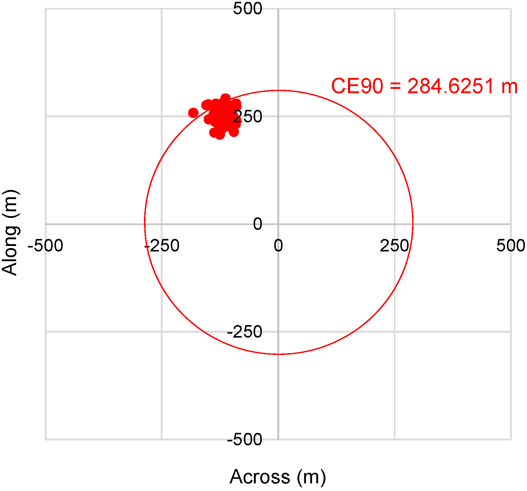
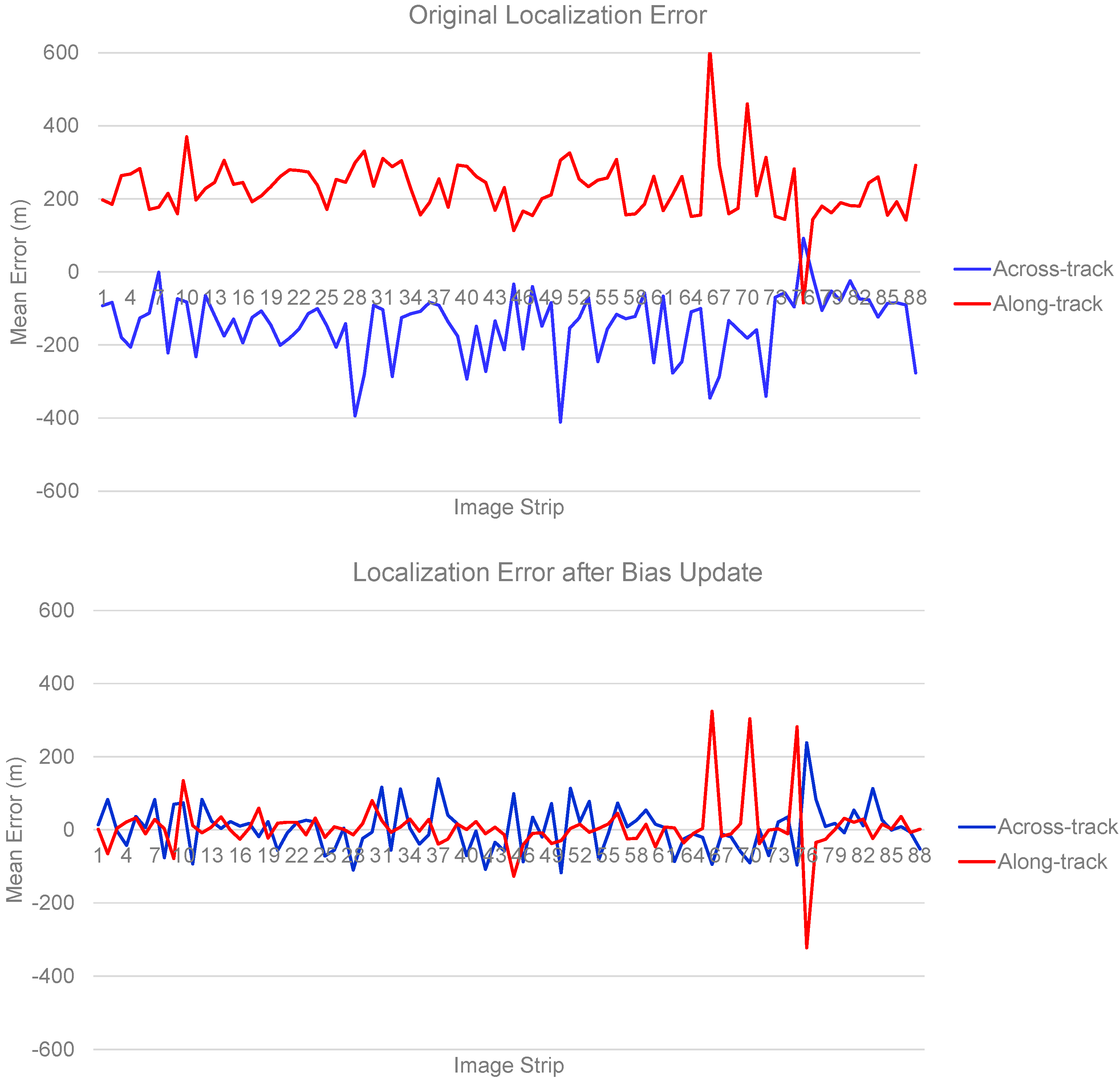
The application of the entire framework was demonstrated by using several tens of real image data covering all operational cases of the satellite in order to prove the feasibility of the proposed framework. The imaging planning decisions and the pattern analysis schemes in the proposed framework provided a guideline for the camera misalignment estimation activity during the initial commissioning period of a high-resolution satellite program. Hundreds of GCPs per image were extracted automatically for camera misalignment estimation. The estimated misalignment was applied to the ground image processor so that the localization error was reduced from 405.97 to 119.33 m in CE90.

The proposed framework is an effective and efficient method to estimate an accurate camera misalignment during a post-launch calibration and validation phase. As it provides precise and reliable measurements and estimation results, it may also reduce the efforts to pre-launch calibration activities. Although this paper focused on the camera misalignment estimation, the presented ideas can be applied to a wide range of applications. The presented GCP extraction algorithm provides many GCPs automatically which can be used for the calibration of other parameters such as focal length, line rate, and image distortion. It can also be attached to the image processing chain to improve the geo-location accuracy of images through a systematic geo-correction using GCPs. The analysis of localization error patterns is useful to discover many other errors such as telemetry error, time drift, gyro scale factor error, and other hardware or software errors of the satellite.

References

1. Müller, R.; Lehner, M.; Reinartz, P. Evaluation of spaceborne and airborne line scanner images using a generic Ortho image processor. In Proceedings of High Resolution Earth Imaging for Geospatial Information, Hannover, Germany, 17–20 May 2005.
2. Tang, X.; Xie, J. Overview of the key technologies for high-resolution satellite mapping. Int. J. Digit. Earth 2012, 5, 228–240. [Google Scholar] [CrossRef]
3. Chen, T.; Shibasaki, R.; Lin, Z. A rigorous laboratory calibration method for interior orientation of an airborne linear push-broom camera. Photogramm. Eng. Remote Sens. 2007, 73, 369–374. [Google Scholar] [CrossRef]
4. Burner, A.W.; Snow, W.L.; Shortis, M.R.; Goad, W.K. Laboratory calibration and characterization of video cameras. Proc. SPIE 1990, 1395, 664–671. [Google Scholar]
5. Liu, T.; Burner, A.W.; Jones, T.W.; Barrows, D.A. Photogrammetric techniques for aerospace applications. Prog. Aerosp. Sci. 2012, 54, 1–58. [Google Scholar] [CrossRef]
6. Radhadevi, P.V.; Solanki, S.S. In-flight geometric calibration of different cameras of IRS-P6 using a physical sensor model. Photogramm. Rec. 2008, 23, 69–89. [Google Scholar] [CrossRef]
7. Bouillon, A.; Bernard, M.; Gigord, P.; Orsoni, A.; Rudowski, V.; Baudoin, A. SPOT 5 HRS geometric performances: Using block adjustment as a key issue to improve quality of DEM generation. ISPRS J. Photogramm. Remote Sens. 2006, 60, 134–146. [Google Scholar] [CrossRef]
8. Breton, E.; Bouillon, A.; Gachet, R.; Delussy, F. Pre-flight and in-flight geometric calibration of SPOT5 HRG and HRS images. ISPRS Int. Arch. Photogramm. Remote Sens. Spat. Inf. Sci. 2002, 34, 20–25. [Google Scholar]
9. Dial, G.; Bowen, H.; Gerlach, F.; Grodecki, J.; Oleszczuk, R. IKONOS satellite, imagery, and products. Remote Sens. Environ. 2003, 88, 23–36. [Google Scholar] [CrossRef]
10. Zhang, C.; Fraser, C.S.; Liu, S. Interior orientation error modelling and correction for precise georeferencing of satellite imagery. Int. Arch. Photogramm. Remote Sens. Spat. Inf. Sci. 2012, 39B1, 285–290. [Google Scholar] [CrossRef]
11. Mulawa, D. On-orbit geometric calibration of the OrbView-3 high resolution imaging satellite. Int. Arch. Photogramm. Remote Sens. Spat. Inf. Sci. 2004, 35, 1–6. [Google Scholar]
12. Leprince, S.; Musé, P.; Avouac, J.-P. In-flight CCD distortion calibration for pushbroom satellites based on subpixel correlation. IEEE Trans. Geosci. Remote Sens. 2008, 46, 2675–2683. [Google Scholar] [CrossRef]
13. Moorthi, S.M.; Kayal, R.; Krishnan, R.R.; Srivastava, P.K. RESOURCESAT-1 LISS-4 MX bands onground co-registration by in-flight calibration and attitude refinement. Int. J. Appl. Earth Obs. Geoinf. 2008, 10, 140–146. [Google Scholar] [CrossRef]
14. Robertson, B.; Beckett, K.; Rampersad, C.; Putih, R. Quantitative geometric calibration & validation of the RapidEye constellation. In Proceeding of the 2009 IEEE International Geoscience and Remote Sensing Symposium, Cape Town, South Africa, 12–17 July 2009.
15. Takaku, J.; Tadono, T. PRISM on-orbit geometric calibration and DSM performance. IEEE Trans. Geosci. Remote Sens. 2009, 47, 4060–4073. [Google Scholar] [CrossRef]
16. Delevit, J.M.; Greslou, D.; Amberg, V.; Dechoz, C.; de Lussy, F.; Lebegue, L.; Latry, C.; Artigues, S.; Bernard, L. Attitude assessment using Pleiades-HR capabilities. Int. Arch. Photogramm. Remote Sens. Spat. Inf. Sci. 2012, 39B1, 525–530. [Google Scholar] [CrossRef]
17. Greslou, D.; de Lussy, F.; Delvit, J.M.; Dechoz, C.; Amberg, V. Pleiades-Hr Innovative Techniques for Geometric Image Quality Commissioning. Int. Arch. Photogramm. Remote Sens. Spat. Inf. Sci. 2012, 39B1, 543–547. [Google Scholar] [CrossRef]
18. De Lussy, F.; Greslou, D.; Dechoz, C.; Amberg, V.; Delvit, J.M.; Lebegue, L.; Blanchet, G.; Fourest, S. Pleiades HR in flight geometrical calibration: Location and mapping of the focal plane. Int. Arch. Photogramm. Remote Sens. Spat. Inf. Sci. 2012, 39, 519–523. [Google Scholar]
19. Wang, M.; Yang, B.; Hu, F.; Zang, X. On-Orbit geometric calibration model and its applications for high-resolution optical satellite imagery. Remote Sens. 2014, 6, 4391–4408. [Google Scholar] [CrossRef]
20. Jiang, Y.; Zhang, G.; Tang, X.; Li, D.; Huang, W. Detection and correction of relative attitude errors for ZY1-02C. IEEE Trans. Geosci. Remote Sens. 2014, 52, 7674–7683. [Google Scholar] [CrossRef]
21. Müller, R.; Krauß, T.; Schneider, M.; Reinartz, P. Automated georeferencing of optical satellite data with integrated sensor model improvement. Photogramm. Eng. Remote Sens. 2012, 78, 61–74. [Google Scholar] [CrossRef]
22. Klančar, G.; Blažič, S.; Matko, D.; Mušič, G. Image-based attitude control of a remote sensing satellite. J. Intell. Robot. Syst. 2011, 66, 343–357. [Google Scholar] [CrossRef]
23. Shi, J.; Tomasi, C. Good features to track. In Proceedings of the IEEE Conference on Computer Vision and Pattern Recognition, Seattle, WA, USA, 21–23 June 1994.
24. Leprince, S.; Barbot, S.; Avouac, J.-P. Automatic and precise orthorectification, coregistration, and subpixel correlation of satellite images, application to ground deformation measurements. IEEE Trans. Geosci. Remote Sens. 2007, 45, 1529–1558. [Google Scholar] [CrossRef]
25. Shuster, M.D. Survey of attitude representations. J. Astronaut. Sci. 1993, 41, 439–517. [Google Scholar]
26. Infinitesimal Rotation. Available online: http://rotations.berkeley.edu/?page_id=1682 (accessed on 15 September 2014).