
An ASIFT-Based Local Registration Method for Satellite Imagery

Abstract
:
1. Introduction
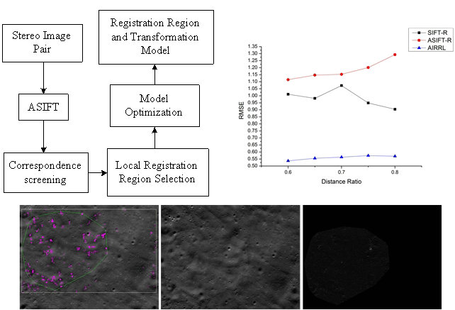
2. Methodology

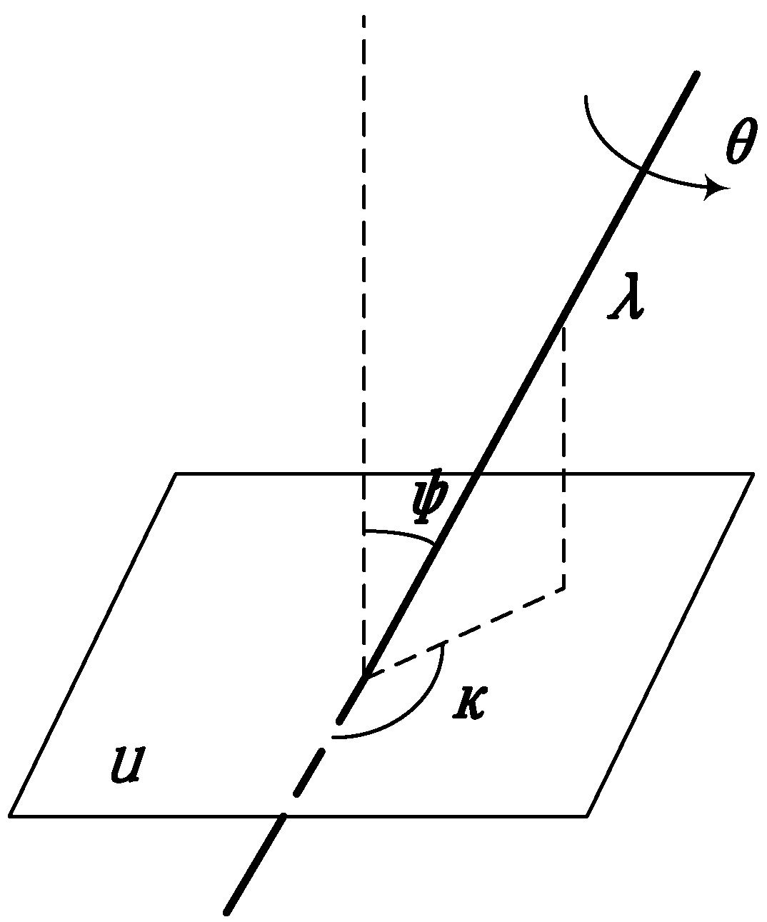
2.1. A Brief Introduction to ASIFT


2.2. Proposed Algorithm
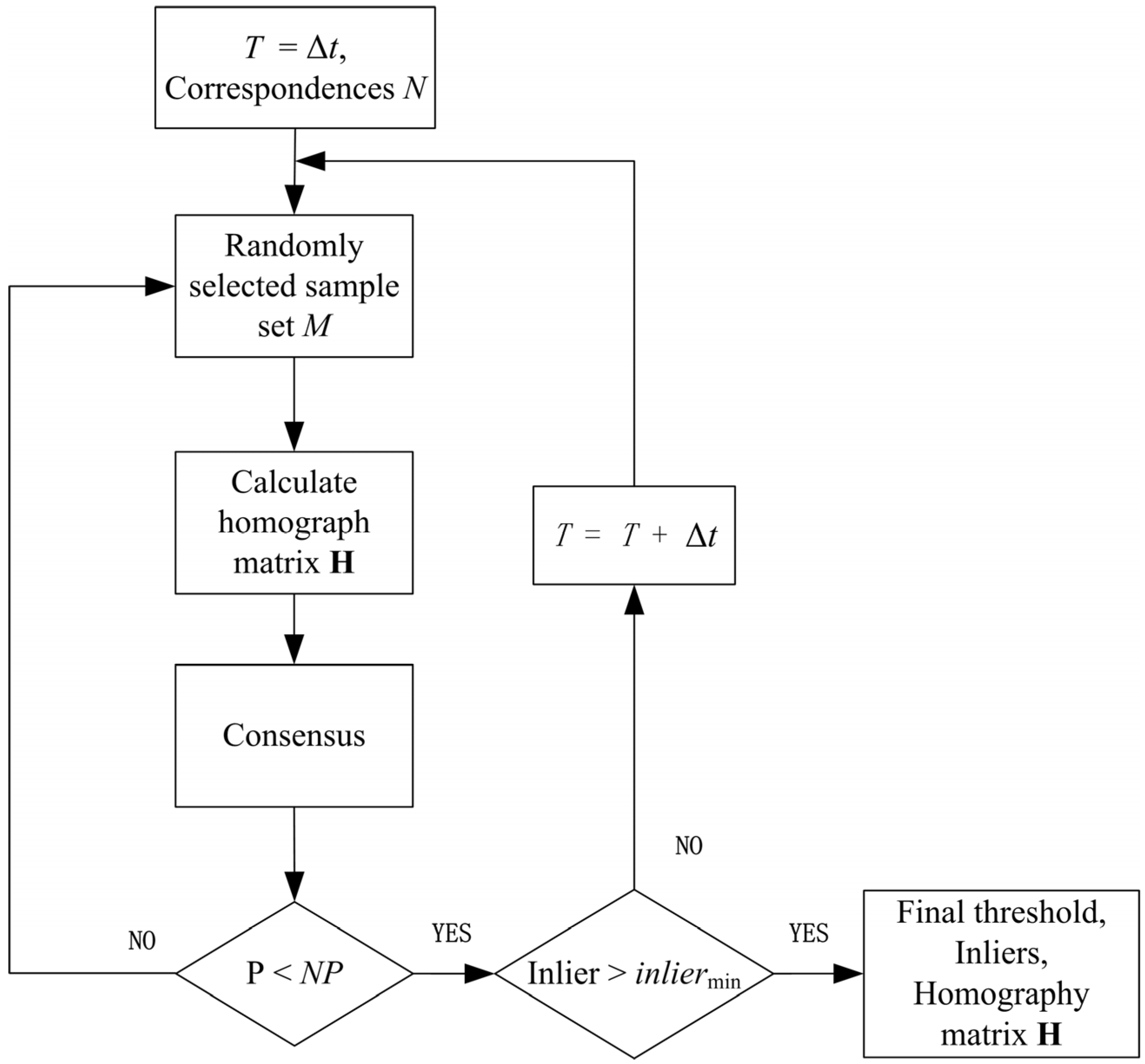
2.2.1. Improved RANSAC

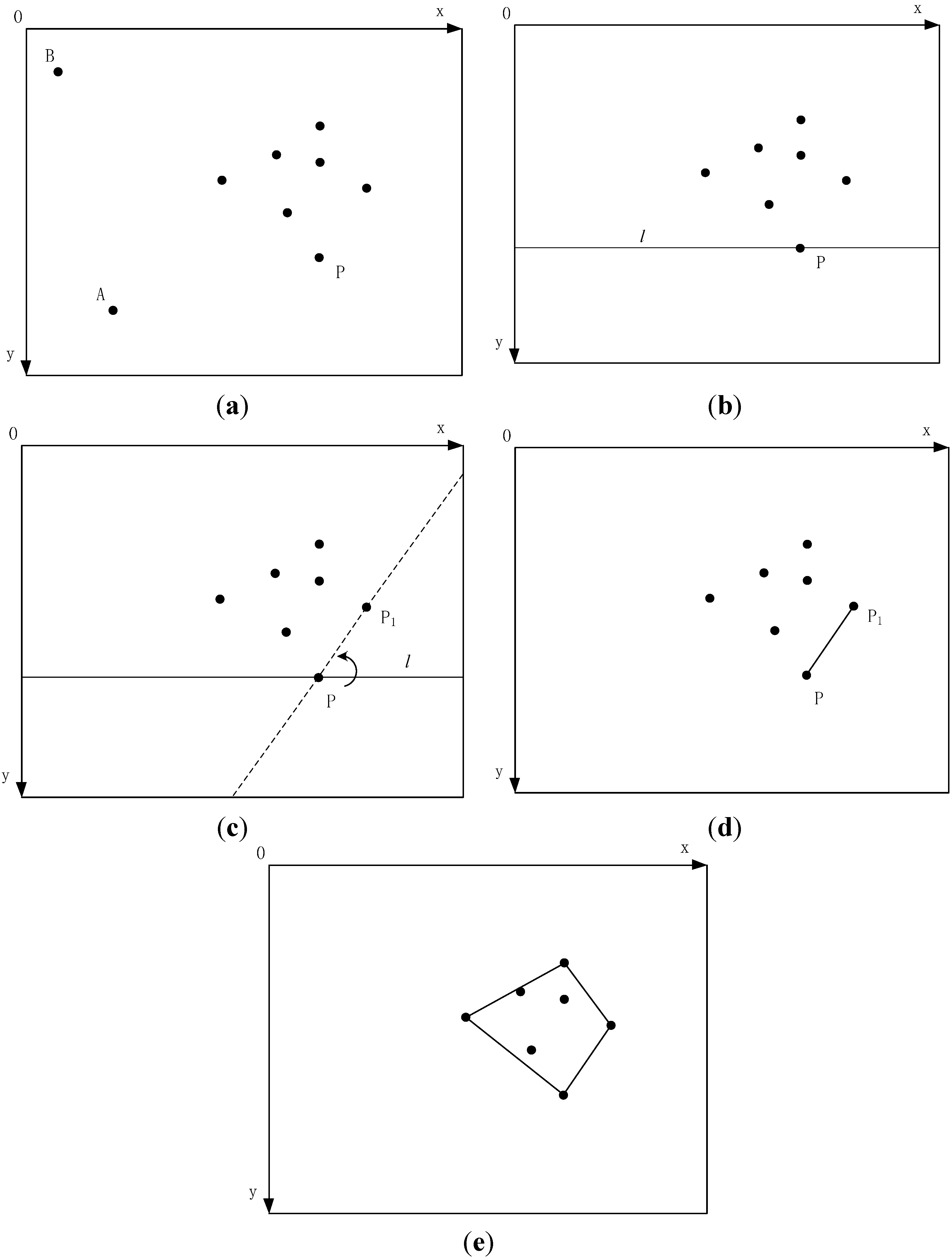
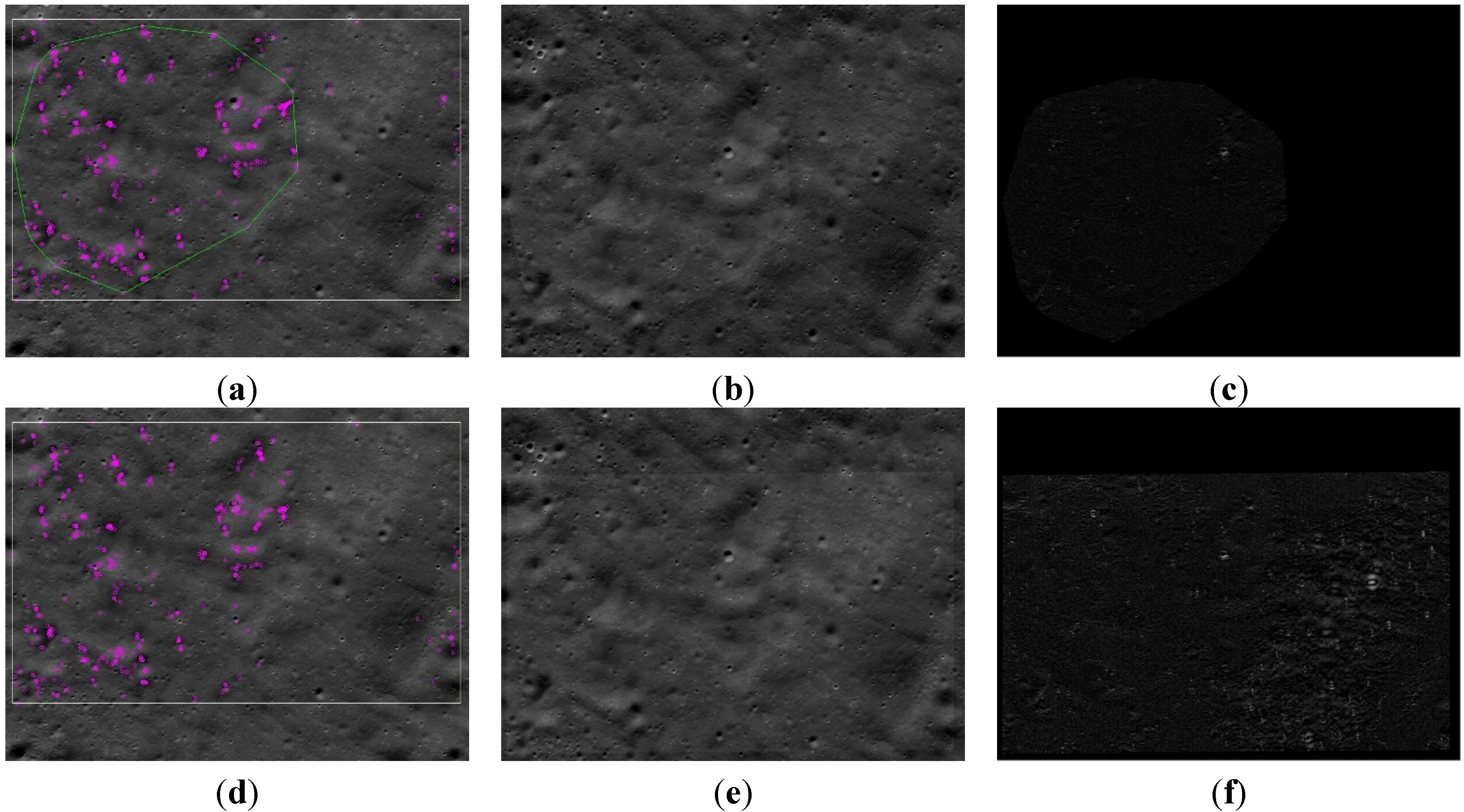
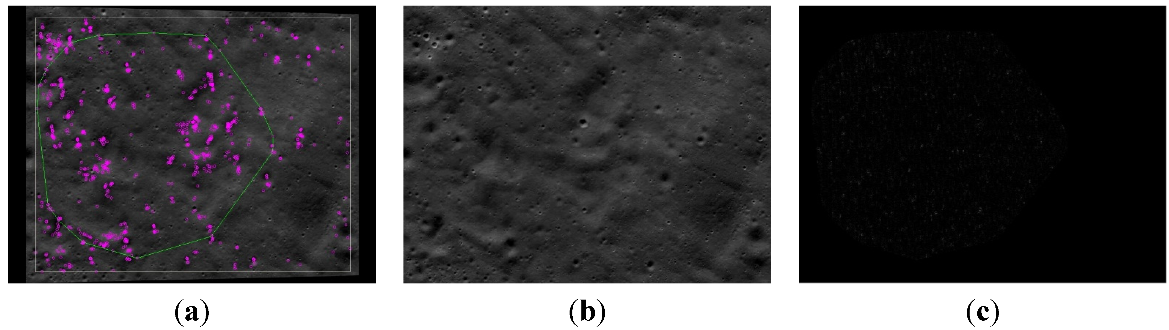
2.2.2. Automatic Selection of Registration Area

2.2.3. LM Optimization
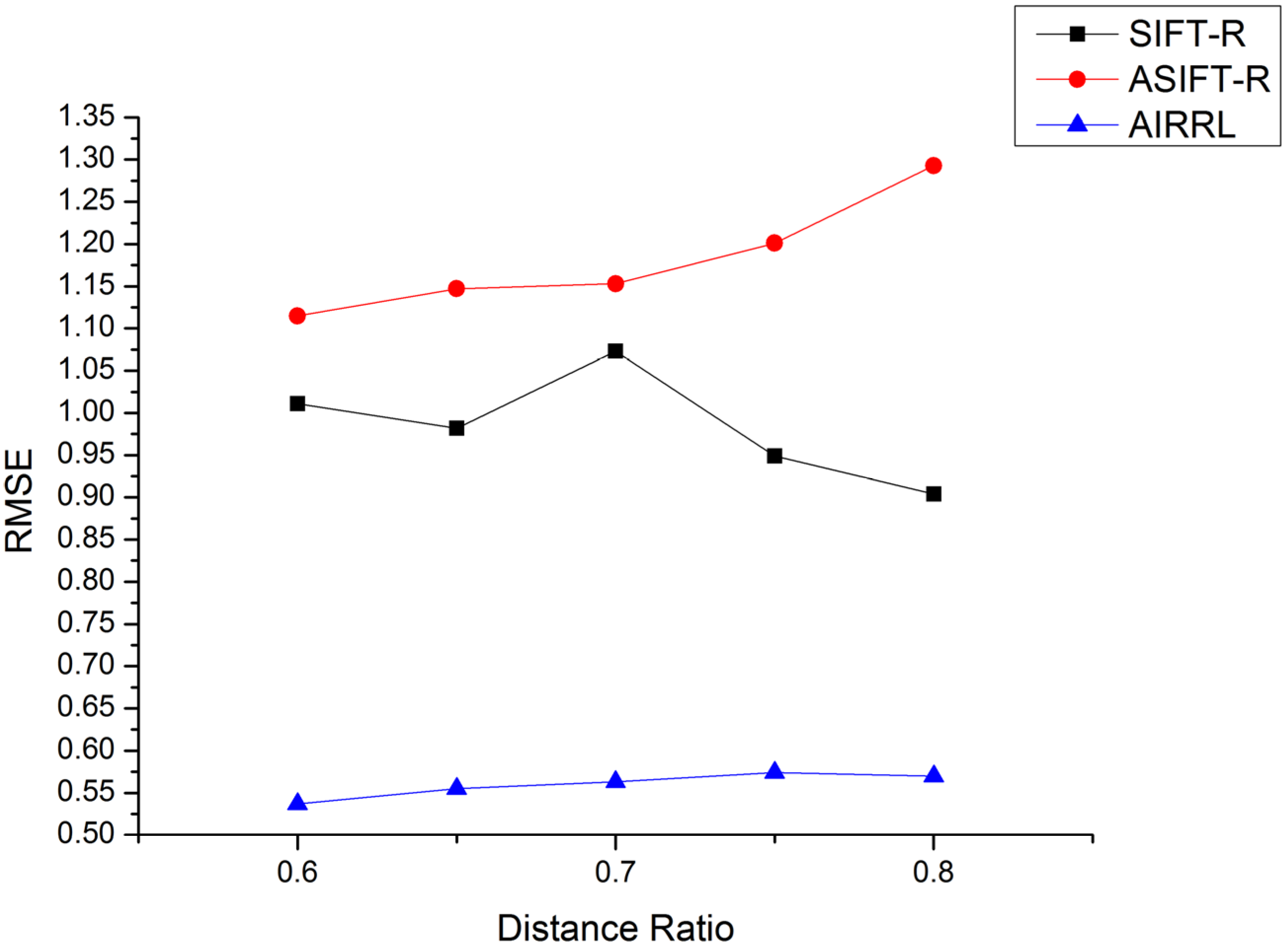
3. Experimental Result and Discussion
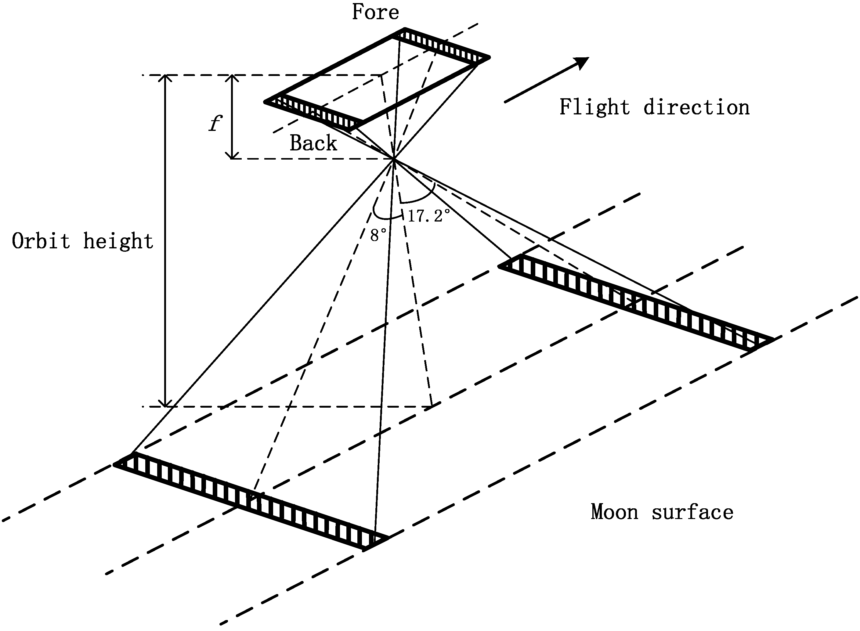
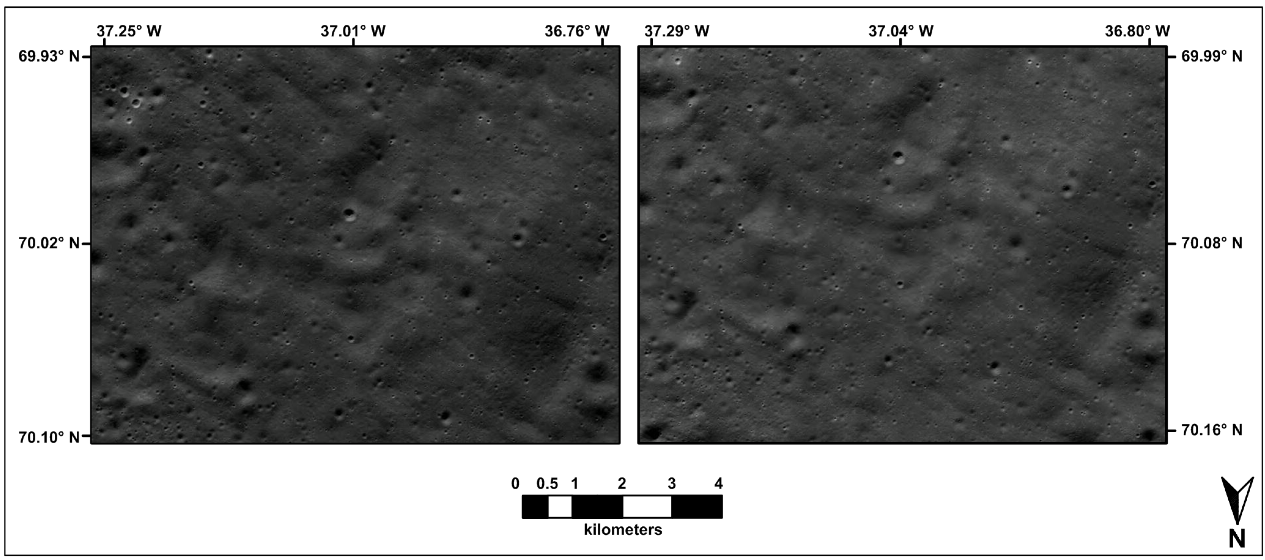
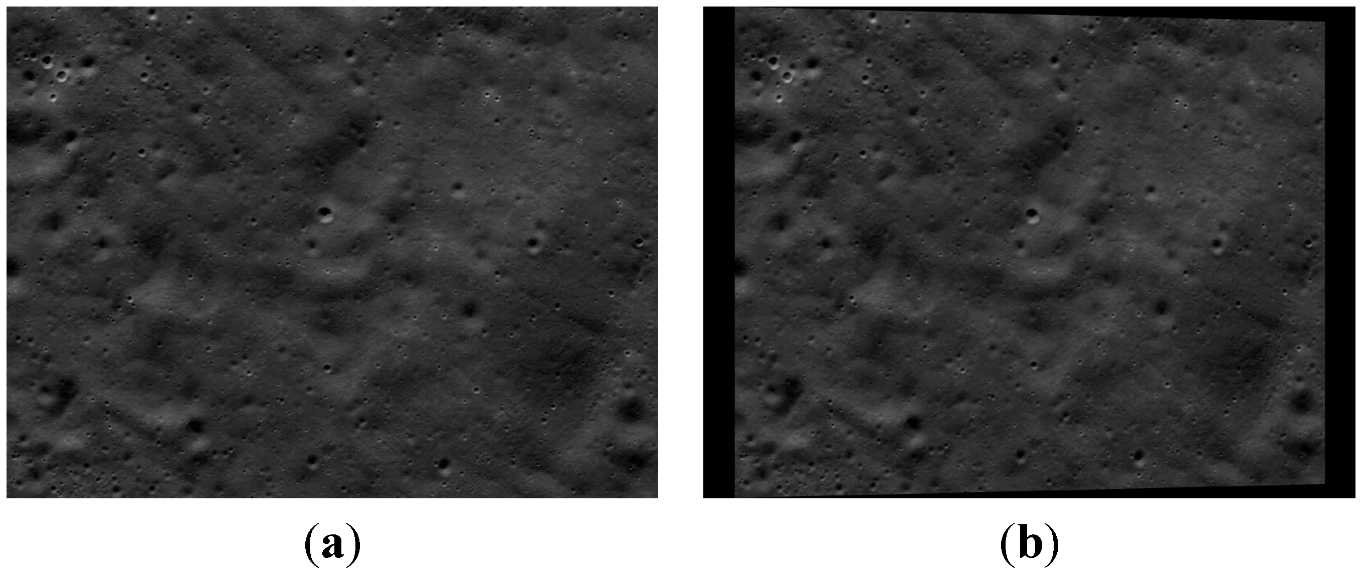
3.1. Source Data Used in the Experiment


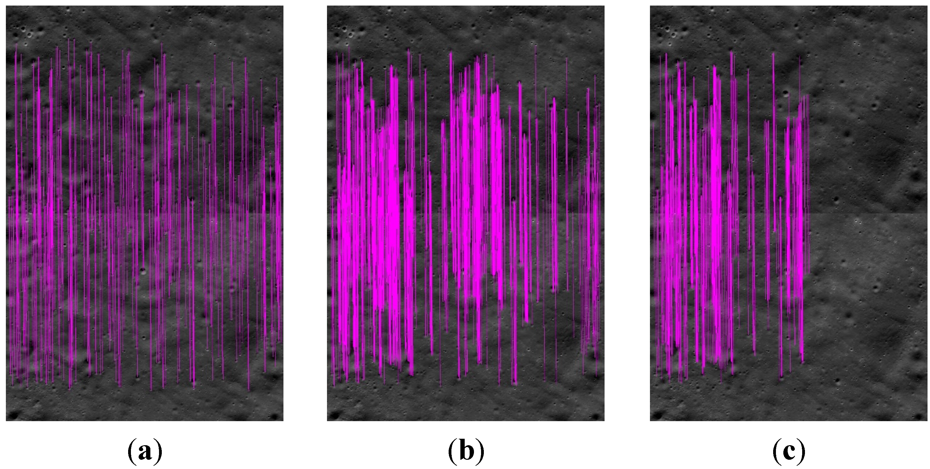
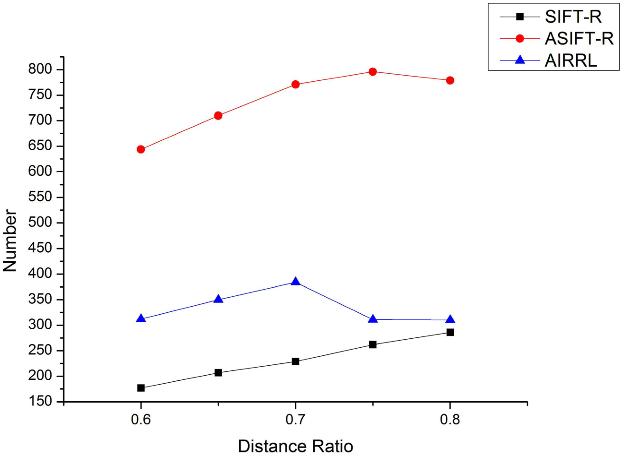
3.2. Discriminative Ability


3.3. Local Registration Region Selection


| Image | I-RMSE |
|---|---|
| Figure 11c | 7.380 |
| Figure 11f | 13.925 |


4. Conclusions
Acknowledgments
Author Contributions
Conflicts of Interest
References
- Zitová, B.; Flusser, J. Image registration methods: A survey. Image Vis. Comput. 2003, 21, 977–1000. [Google Scholar] [CrossRef]
- Lemmens, M.J.P.M. A survey on stereo matching techniques. Int. Arch. Photogramm. Remote Sens. Spat. Inf. Sci. 1988, 27, 11–23. [Google Scholar]
- Hui-Zhong, C.; Ning, J.; Jun, W.; Yong-Guang, C.; Luo, C. A novel saliency detection method for lunar remote sensing images. IEEE Geosci. Remote Sens. Lett. 2014, 11, 24–28. [Google Scholar]
- Hussain, M.; Chen, D.M.; Cheng, A.; Wei, H.; Stanley, D. Change detection from remotely sensed images: From pixel-based to object-based approaches. ISPRS J. Photogramm. Remote Sens. 2013, 80, 91–106. [Google Scholar] [CrossRef]
- Lucchese, L.; Leorin, S.; Cortelazzo, G.M. Estimation of two-dimensional affine transformations through polar curve matching and its application to image mosaicking and remote-sensing data registration. IEEE Trans. Image Process. 2006, 15, 3008–3019. [Google Scholar] [CrossRef] [PubMed]
- Dai, X.; Siamak, K. The effects of image misregistration on the accuracy of remotely sensed change detection. IEEE Trans. Geosci. Remote Sens. 1998, 36, 1566–1577. [Google Scholar]
- Townshend, J.R.G.; Justice, C.O.; Gurney, C.; McManus, J. The impact of misregistration on change detection. IEEE Trans. Geosci. Remote Sens. 1992, 30, 1054–1060. [Google Scholar] [CrossRef]
- Ton, J.; Jain, A.K. Registering landsat images by point matching. IEEE Trans. Geosci. Remote Sens. 1989, 27, 642–651. [Google Scholar] [CrossRef]
- Goshtasby, A.A. Feature selection. In 2-D and 3-D Image Registration; John Wiley & Sons, Inc.: Hoboken, NJ, USA, 2005; pp. 43–61. [Google Scholar]
- Yi, Z.; Zhiguo, C.; Yang, X. Multi-spectral remote image registration based on SIFT. Electron. Lett. 2008, 44, 107–108. [Google Scholar] [CrossRef]
- Lowe, D. Distinctive image features from scale-invariant keypoints. Int. J. Comput. Vis. 2004, 60, 91–110. [Google Scholar] [CrossRef]
- Lowe, D.G. Object recognition from local scale-invariant features. In Proceedings of the 7th IEEE International Conference on Computer Vision, Kerkyra, Greece, 20–27 Septrmber 1999; Volume 2, pp. 1150–1157.
- Goncalves, H.; Corte-Real, L.; Goncalves, J.A. Automatic image registration through image segmentation and SIFT. IEEE Trans. Geosci. Remote Sens. 2011, 49, 2589–2600. [Google Scholar] [CrossRef]
- Gong, M.; Zhao, S.; Jiao, L.; Tian, D.; Wang, S. A novel coarse-to-fine scheme for automatic image registration based on SIFT and mutual information. IEEE Trans. Geosci. Remote Sens. 2014, 52, 4328–4338. [Google Scholar]
- Cai, G.-R.; Jodoin, P.-M.; Li, S.-Z.; Wu, Y.D.; Su, S.-Z.; Huang, Z.K. Perspective-SIFT: An efficient tool for low-altitude remote sensing image registration. Signal Process. 2013, 93, 3088–3110. [Google Scholar] [CrossRef]
- Zhu, Y.; Cheng, S.; Stanković, V.; Stanković, L. Image registration using BP-SIFT. J. Vis. Commun. Image Represent. 2013, 24, 448–457. [Google Scholar] [CrossRef]
- Morel, J.-M.; Yu, G. Asift: A new framework for fully affine invariant image comparison. SIAM J. Imaging Sci. 2009, 2, 438–469. [Google Scholar] [CrossRef]
- Ting, H.; Hongyan, Z.; Huanfeng, S.; Liangpei, Z. Robust registration by rank minimization for multiangle hyper/multispectral remotely sensed imagery. IEEE J. Sel. Top. Appl. Earth Observ. Remote Sens. 2014, 7, 2443–2457. [Google Scholar]
- Fischler, M.A.; Bolles, R.C. Random sample consensus: A paradigm for model fitting with applications to image analysis and automated cartography. Commun. ACM 1981, 24, 381–395. [Google Scholar] [CrossRef]
- Hartley, R.; Zisserman, A. Multiple View Geometry in Computer Vision; Cambridge University Press: Cambridge, UK, 2003; p. 700. [Google Scholar]
- Chum, O.; Matas, J. Matching with PROSAC—Progressive sample consensus. In Proceedings of the 2005 IEEE Computer Society Conference on Computer Vision and Pattern Recognition (CVPR), San Diego, CA, USA, 20–26 June 2005; Volume 1, pp. 220–226.
- Brown, M.; Lowe, D.G. Rcognising panoramas. In Proceedings of the 9th IEEE International Conference on Computer Vision (ICCV), Nice, France, 13–16 October 2003; pp. 1218–1227.
- Marquardt, D.W. An algorithm for least-squares estimation of nonlinear parameters. J. Soc. Ind. Appl. Math. 1963, 11, 431–441. [Google Scholar] [CrossRef]
- Zhao, B.; Yang, J.; Wen, D.; Gao, W.; Chang, L.; Song, Z.; Xue, B.; Zhao, W. Overall scheme and on-orbit images of Chang’E-2 lunar satellite CCD stereo camera. Sci. China Technol. Sci. 2011, 54, 2237–2242. [Google Scholar] [CrossRef]
- Bin, F.; Chunlei, H.; Chunhong, P.; Qingqun, K. Registration of optical and sar satellite images by exploring the spatial relationship of the improved SIFT. IEEE Geosci. Remote Sens. Lett. 2013, 10, 657–661. [Google Scholar] [CrossRef]
- Hans, R. Opensift. Available online: http://robwhess.github.io/opensift/ (accessed on 12 March 2015).
- Yu, G.; Morel, J.-M. Asift: An Algorithm for Fully Affine Invariant Comparison. Available online: http://www.ipol.im/pub/art/2011/my-asift/ (accessed on 12 March 2015).
- Mikolajczyk, K.; Schmid, C. A performance evaluation of local descriptors. IEEE Trans. Pattern Anal. Mach. Intell. 2005, 27, 1615–1630. [Google Scholar] [CrossRef] [PubMed]
© 2015 by the authors; licensee MDPI, Basel, Switzerland. This article is an open access article distributed under the terms and conditions of the Creative Commons Attribution license (http://creativecommons.org/licenses/by/4.0/).
Share and Cite
Wang, X.; Li, Y.; Wei, H.; Liu, F. An ASIFT-Based Local Registration Method for Satellite Imagery. Remote Sens. 2015, 7, 7044-7061. https://0-doi-org.brum.beds.ac.uk/10.3390/rs70607044
Wang X, Li Y, Wei H, Liu F. An ASIFT-Based Local Registration Method for Satellite Imagery. Remote Sensing. 2015; 7(6):7044-7061. https://0-doi-org.brum.beds.ac.uk/10.3390/rs70607044
Chicago/Turabian StyleWang, Xiangjun, Yang Li, Hong Wei, and Feng Liu. 2015. "An ASIFT-Based Local Registration Method for Satellite Imagery" Remote Sensing 7, no. 6: 7044-7061. https://0-doi-org.brum.beds.ac.uk/10.3390/rs70607044