A Least Squares Collocation Method for Accuracy Improvement of Mobile LiDAR Systems

Abstract

In environments that are hostile to Global Navigation Satellites Systems (GNSS), the precision achieved by a mobile light detection and ranging (LiDAR) system (MLS) can deteriorate into the sub-meter or even the meter range due to errors in the positioning and orientation system (POS). This paper proposes a novel least squares collocation (LSC)-based method to improve the accuracy of the MLS in these hostile environments. Through a thorough consideration of the characteristics of POS errors, the proposed LSC-based method effectively corrects these errors using LiDAR control points, thereby improving the accuracy of the MLS. This method is also applied to the calibration of misalignment between the laser scanner and the POS. Several datasets from different scenarios have been adopted in order to evaluate the effectiveness of the proposed method. The results from experiments indicate that this method would represent a significant improvement in terms of the accuracy of the MLS in environments that are essentially hostile to GNSS and is also effective regarding the calibration of misalignment.

1. Introduction

The mobile light detection and ranging (LiDAR) system (MLS), in which positioning and orientation systems (POS) and laser scanners are integrated, has become one of the key instruments used in modern surveying and mapping engineering due to its high precision, convenience, efficiency and effectiveness. The point clouds generated by the MLS are widely applied to the construction of Digital Earth, smart cities, and so on. For these practical applications, accuracy is always paramount.

The accuracy assessment and control technologies for the MLS can be classified as data driven or model driven. Data-driven technologies directly correct the LiDAR point clouds using ground control points (GCPs). Csanyi and Toth [1] designed a kind of circular LiDAR control target that is easy to extract from point clouds. In their method, a strip adjustment procedure was adopted to correct the absolute errors. Toth et al. [2] used pavement markings as ground control for the accuracy assessment and control of LiDAR data. They adopted the iterative closest point (ICP) [3] algorithm to calculate the transformation parameters from LiDAR points to control points. Fowler and Kadatskiy [4] improved the accuracy of airborne LiDAR and ground mobile LiDAR data through the control of high-precision and high-resolution terrestrial LiDAR data. Wu et al. [5] used 12 parameter affine transformation to improve the accuracy of LiDAR data. These data-driven methods directly correct point cloud data by rigid transformation of coordinates. The performance of data-driven methods relies on many factors, such as the number of GCPs and their distribution, the properties of targets, and so on. Points with similar coordinates in the LiDAR coordinate system and similar errors with respect to control points would represent a significant improvement in terms of accuracy, but would achieve little in other respects. This feature can be found in the results of experiments conducted by Csanyi and Toth [1] and Wu et al. [5].

Some researchers have developed model-driven methods as an alternative. Model-driven technology analyses the error sources in the MLS and their impact on LiDAR points and then proposes methods for the elimination and reduction of these errors, ultimately overcoming the problems in the data-driven technology. Habib et al. [6] pointed out the error budget of LiDAR systems and analysed possible random and systematic errors and their impact on LiDAR points. In their analysis, the positioning and orientation errors were regarded as noise, and the misalignment between laser scanners and the POS was seen as a systematic error. Burman [7] proposed a strip adjustment procedure for the correction of misalignment based on the MLS error model. Although their method had no need for GCPs, it needed to scan an area with height or intensity gradients three times and in different directions. If GCPs are used to correct misalignment, the operation becomes simpler. Pothou et al. [8] used photogrammetrically-restituted buildings as “reference points” to calculate misalignment. In both [7] and [8], positioning and orientation errors were regarded as random noise. Ye et al. [9] proposed a GCP-based misalignment calibration method, in which positioning and orientation errors were regarded as constant systematic errors and corrected. However, the method of Ye et al. [9] has not been applied to POS correction in complex environments where positioning and orientation errors cannot be treated as constants.

Although model-driven technology aims to eliminate sources of error, most current model-driven methods emphasize the correction of misalignment between the POS and the laser scanner, but ignore errors in the POS. The promising results of Ye et al. [9] indicate the necessity for further research in terms of the reduction of POS errors. POS errors are, in some cases, the main source of error in the MLS. According to both the literature and experiments, LiDAR point clouds can achieve sub-decimetre and centimetre precision [1,10–17] under good GNSS visibility conditions, but this accuracy is likely to decrease dramatically in sub-meter or meter ranges [10,12,16] when the GNSS signal is blocked by buildings or areas of dense woodland and also when a severe multi-path effect occurs. The POS is composed of a set of GNSS and a set of inertial measurement units (IMU). To improve the reliability and accuracy of a POS in environments hostile to GNSS, a direct solution would be to adopt a high-grade IMU, such as a laser IMU. There are, however, two limitations to this solution. Firstly, most high-grade IMUs are too expensive for ordinary civilian applications, and secondly, it is impossible to maintain the absolute accuracy of POS with a high-grade IMU during prolonged periods in conditions unfavourable to GNSS. Thus, the maintenance of a high degree of accuracy in the MLS in all kinds of environment becomes a key problem in terms of their application. In the fields of automation and robotics, some researchers proposed simultaneous localization and mapping (SLAM)-aided GNSS/INS methods under GNSS-blockage conditions [18–20]. SLAM uses cameras or 3D laser scanners or rotating 2D laser scanners to calculate the trajectory of vehicles through four steps: data association, map matching, loop detection and global optimization. On the contrary, most of the MLS uses 2D laser scanners, which are fixed on the vehicle. There is no overlapped part between two neighbouring frames. Additionally, the localization accuracy of SLAM is usually in sub-meters or meters. Therefore, in the field of MLS, SLAM is not a proper solution, because of the sensors setup and the requirement of accuracy.

In order to improve the accuracy of the MLS in environments where GNSS visibility is poor, a novel method for the correction of POS errors using LiDAR control points is put forward in this paper. This method is based on the least squares collocation (LSC; [21,22]) theory, which has been proven to be an effective method for the handling of errors in GNSS/inertial navigation system (INS) levelling ([23]). This method is based on the MLS error model presented in [6,7] and investigates the characteristics of POS errors very thoroughly. This LSC model can also be used to handle the problem of misalignment.

The rest of the article is organized as follows: Section 2 reviews the MLS error model and analyses the characteristics of POS errors first of all; the LSC models are presented in order to correct POS errors and misalignment. Section 3 validates the proposed models using several datasets. The discussion and conclusions are provided in Section 4.

2. Method

2.1. Definition of Coordinate Systems

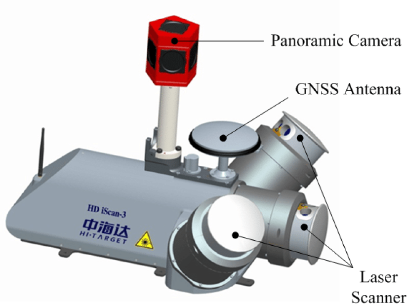
In the MLS, there are three coordinate systems (Figure 1):

• the geo-spatial coordinate system (GCS);
• the POS body coordinate system (PCS);
• the laser scanner coordinate system (LCS).

The GCS is usually the Gauss coordinate system in which the X axis points to the east, the Y axis to the north and the Z axis up. The coordinates of LiDAR point clouds and control points fall under this coordinate system. The PCS is a right-handed system and is attached to the IMU: the origin is located in the IMU navigation centre, with the X axis pointing to the right, the Y axis pointing forward and the Z axis pointing up. The LCS is also a right-handed system in which the X axis overlaps with the zero-degree laser beam, the Y axis is perpendicular to the X axis in the scanning plane and the Z axis is perpendicular to the scanning plane. The relationship between these coordinate systems is shown in Figure 1.

The raw data of the laser scanner were in the LCS and then transformed into the PCS with spatial alignment parameters, including three translations and three rotations, and, finally, transformed into the GCS with the position and orientation measured by the POS. The final MLS dataset represents millions of points with three-dimensional coordinates in the GCS.

2.2. Error Model of the MLS

The formula used to calculate the LiDAR point is given in Equation (1):

$$X_G=T_G+R_P^G\cdot (R_L^P\cdot X_L+T_L^P)$$

(1)

where the subscripts G, P, L indicate the GCS, PCS and LCS coordinate systems, respectively, X_G is the coordinate vector of the LiDAR point in the GCS, T_G = [T_E, T_N, T_H ]^T is the coordinate vector of the POS navigation centre in the GCS, $R_P^G$ is the rotation matrix from the PCS to GCS constituted from the orientation o(o = [γ, ρ, ϕ]^T, γ roll, ρ pitch, ϕ heading), X_L is the coordinate vector of the laser scanner measurement in the LCS, $T_L^P={[T_x,T_y,T_z]}^T$ is the translation vector from the LCS to the PCS and $R_L^P$ is the rotation matrix constituted from the alignment angles (θ = [θ_x, θ_y, θ_z ]^T). Owing to the fact that there are errors in every measurement and calibration parameter, Equation (1) becomes Equation (2) by adding error vectors:

$$X_G+\mathrm{\Delta }{X}_G=T_G+\mathrm{\Delta }{T}_G+(I+\mathrm{\Delta }{R}_P^G)\cdot R_P^G\cdot ((I+\mathrm{\Delta }{R}_L^P)\cdot R_L^P\cdot (X_L+\mathrm{\Delta }{X}_L)+T_L^P+\mathrm{\Delta }{T}_L^P)$$

(2)

where the variable with the Δ prefix denotes the error vector of the corresponding variable and I denotes the identity matrix. Specifically:

$$\begin{array}{l}\mathrm{\Delta }{R}_P^G=\mathrm{\Phi }(\mathrm{\Delta }o)=\left[\begin{array}{ccc}0& -\mathrm{\Delta }\varphi & \mathrm{\Delta }\rho \\ \mathrm{\Delta }\varphi & 0& -\mathrm{\Delta }\gamma \\ -\mathrm{\Delta }\rho & \mathrm{\Delta }\gamma & 0\end{array}\right]\\ \mathrm{\Delta }{R}_L^P=\mathrm{\Phi }(\mathrm{\Delta }\theta )\left[\begin{array}{ccc}0& -\mathrm{\Delta }{\theta }_z& \mathrm{\Delta }{\theta }_y\\ \mathrm{\Delta }{\theta }_z& 0& -\mathrm{\Delta }{\theta }_x\\ -\mathrm{\Delta }{\theta }_y& \mathrm{\Delta }{\theta }_x& 0\end{array}\right]\end{array}$$

(3)

Here, Φ(·) is a function transforming a vector to a matrix as follows:

$$\mathrm{\Phi }\left(\left[\begin{array}{c}x\\ y\\ z\end{array}\right]\right)=\left[\begin{array}{ccc}0& -z& y\\ z& 0& -x\\ -y& x& 0\end{array}\right]$$

(4)

Ignoring second order small quantities, the MLS error model can be deduced as Equation (5):

$$\begin{array}{l}\mathrm{\Delta }{X}_G=\underset{}{\underbrace{\mathrm{\Delta }{T}_G+\mathrm{\Delta }{R}_P^G\cdot R_P^G\cdot (R_L^P\cdot X_L+T_L^P)}}\\ +\underset{}{\underbrace{R_P^G\cdot \mathrm{\Delta }{R}_L^P\cdot R_L^P\cdot X_L+R_P^G\mathrm{\Delta }{T}_L^P}}+\underset{}{\underbrace{R_P^G\cdot R_L^P\cdot \mathrm{\Delta }{X}_L}}\end{array}$$

(5)

Equation (5) shows that the whole MLS error consists of three parts: the first part is the POS error, including positioning error ΔT_G and orientation error Δo; the second part represents calibration errors, i.e., misalignment, including $\mathrm{\Delta }{T}_L^P$ and Δθ; and the third part is the laser scanning error, including ranging and scanning angle errors.

In the analysis of the error budget of the LiDAR systems in [6], misalignment is regarded as a systematic error, while the POS error and laser scanning error are seen merely as random noise. However, as far as the accuracy improvement for the MLS in an environment unfavourable to GNSS is concerned, a more dedicated POS error model is needed.

2.3. POS Error

In GNSS/IMU integration systems, short-term accuracy depends on the IMU and long-term on the GNSS [24]. Between two neighbouring GNSS epochs, the position and orientation calculated with inertial data, that is gyroscope data and accelerometer data, change both smoothly and consistently. However, there are cumulative errors here also. These errors are corrected at each GNSS epoch, but the trajectory becomes inconsistent. Therefore, after filtering with an extended Kalman filter (EKF; [25]), in most GNSS/IMU solution software, the initial trajectory is corrected with smoothers, such as the forward-backward smoother or Rauch–Tung–Striebel (R-T-S; [26]) smoother to keep the trajectory consistent. The smoother takes the filtering information to calculate the residual correction for each point. Therefore, after the smoothing process, the random error, both with regard to positioning and orientation, becomes time correlated.

It is interesting to explore the performance of positioning and orientation errors in environments inimical to GNSS further. Without GNSS correction, the positioning and orientation errors would accumulate with time. As far as accumulated errors in the orientation are concerned, they can be corrected with accurate GNSS Doppler measurements when the GNSS signal is available, irrespective of whether the GNSS signal is good or bad. Thus, the orientation error Δo can be regarded as a kind of random error. Additionally, as far as the accumulated errors in the positioning are concerned, these will be corrected only when the GNSS is good. In environments hostile to GNSS, its precision and accuracy decrease, so that the accumulated positioning errors will not be completely eliminated and positioning bias will occur. Since the smoothing process makes the POS trajectory consistent and smooth, the positioning error ΔT_G changes with time, thus showing a kind of tendency variable. Ultimately, the positioning error contains a tendency error, as well as a random error.

2.4. The Least Squares Collocation Model

2.4.1. The Basic Principles of Least Squares Collocation

Least squares collocation is a method by which the fitting problem with tendency variables and random variables can be solved, unlike classical least squares methods, in which the randomness of variables is not taken into account. In other words, there are only tendency variables in least squares (LS) problems. A typical observation equation with respect to the LSC model is as follows:

$$L=AY+B\mathrm{\Lambda }+\mathrm{\delta }$$

(6)

Here, L is the observation vector, Y is the vector of tendency variables, Λ is the vector of random variables of observed sites, δ is the measurement noises and A and B are the design matrices of Y and Λ. The vector of random variables of other sites is denoted by Λ′. Λ′ is spatially or temporally correlated to Λ. There is clearly no BΛ in the observation equation of the LS model. The LSC solution not only estimates the value of tendency variables Y, but also estimates the value of random variables Λ and Λ′.

2.4.2. The Least Squares Collocation Model for the Correction of POS Error

If alignment parameters from the LCS to the PCS have been calibrated accurately in advance and the ranging and angle errors of the laser scanners are small, the second and the third parts in Equation (5) will be treated as random noise and are both denoted by δ. The tendency variable of the positioning error ΔT_G is denoted by ΔT, the random variable of ΔT_G by Λ_T and the random variable of orientation error Δo by Λ_o. Then, Equation (5) can be modified to Equation (7):

$$\mathrm{\Delta }{X}_G=A^{\prime }\mathrm{\Delta }T+[B_T,B_o]\cdot [\begin{array}{c}{\mathrm{\Lambda }}_T\\ {\mathrm{\Lambda }}_o\end{array}]+\mathrm{\delta }$$

(7)

where A′ = I is the coefficient matrix of tendency variable ΔT, B_T = I is the coefficient matrix of Λ_T and B_o is the coefficient matrix of Λ_o. ΔX_G is the vector of the coordinate difference between the control points and their corresponding LiDAR points. To deduce the specific representation of B_o, an intermediate variable $\widehat{G}$ is introduced:

$$\widehat{G}=R_P^G\cdot (R_L^P\cdot X_L+T_L^P)={[G_x,G_y,G_z]}^T$$

(8)

Then, we can get:

$$\mathrm{\Delta }{R}_P^G\cdot \widehat{G}=-\mathrm{\Phi }(G)\mathrm{\Delta }o$$

(9)

Thus, the representation of B_o is:

$$B_o=\left[\begin{array}{ccc}0& -G_Z& G_y\\ G_Z& 0& -G_x\\ -G_y& G_x& 0\end{array}\right]=-\mathrm{\Phi }(\widehat{G})$$

(10)

The tendency variables of positioning errors with respect to the east, north and height are all modelled as an n-th-order polynomial varying over time.

$$\mathrm{\Delta }T=\left[\begin{array}{c}{a}_0+a_{1}t+\dots +a_n{t}^n\\ b_0+b_{1}t+\dots +b_n{t}^n\\ c_0+c_{1}t+\dots +c_n{t}^n\end{array}\right]=CY$$

(11)

where Y = [a₀, a₁, …, a_n, b₀, b₁, …, b_n, c₀, c₁, …, c_n]^T and C is the corresponding time-variant coefficient. Let B = [B_T, B_o] and Λ = [Λ_T, Λ_o]^T ; then Equation (7) becomes Equation (12):

$$\begin{array}{r}\mathrm{\Delta }{X}_G=A^{\prime }CY+B\mathrm{\Lambda }+\mathrm{\delta }\\ =AY+B\mathrm{\Lambda }+\mathrm{\delta }\end{array}$$

(12)

where A = A′C. According to the LSC theory ([22]), the tendency and random variables can be solved when more than n + 1 LiDAR control points are observed.

$$\widehat{\mathrm{Y}}={\{{\mathrm{A}}^T{({\mathrm{BD}}_{\mathrm{\Lambda }}{\mathrm{B}}^T+\mathrm{D}\omega )}^{-1}\text{A}\}}^{-1}{\mathrm{A}}^T{({\mathrm{BD}}_{\mathrm{\Lambda }}{\mathrm{B}}^T+\mathrm{D}\omega )}^{-1}{\mathrm{\Delta }\text{X}}_{\mathrm{G}}$$

(13)

$$\widehat{\mathrm{\Lambda }}={\mathrm{D}}_{\mathrm{\Lambda }}{\mathrm{B}}^T{({\mathrm{BD}}_{\mathrm{\Lambda }}{\mathrm{B}}^T+{\mathrm{D}}_{\omega })}^{-}{}^1(\mathrm{\Delta }{\mathrm{X}}_{\mathrm{G}}-\mathrm{A}\widehat{\mathrm{Y}})$$

(14)

where D_Λ is the priori covariance matrix of Λ and D_ω is the covariance matrix of δ. The random variables of other epochs Λ′ are calculated by Equation (15),

$$\widehat{\mathrm{\Lambda }}\prime ={\mathrm{D}}_{{\mathrm{\Lambda }}^{\prime }\mathrm{\Lambda }}{\mathrm{B}}^T{({\mathrm{BD}}_{\mathrm{\Lambda }}{\mathrm{B}}^T{+\text{D}}_{\omega })}^{-1}(\mathrm{\Delta }{\mathrm{X}}_{\mathrm{G}}-\mathrm{A}\widehat{\mathrm{Y}})$$

(15)

where D_{Λ′ Λ} is the covariance matrix between the random variables of control epochs and the other epochs to be corrected (that is, the interpolated epoch).

2.4.3. The Least Squares Collocation Model for Misalignment Calibration

In Section 2.4.2, the alignment parameters between the LCS and the PCS are assumed to have been calibrated accurately in advance. However, this is not always the case. The way in which these parameters are calculated is another important issue in the MLS. This section presents a new calibration method based on the proposed LSC model. In this section, the GNSS signal is assumed to be adequate. The misalignment parameters are treated as time-invariant tendency variables denoted by $Y={\left[\mathrm{\Delta }{T}_L^P,\mathrm{\Delta }\theta \right]}^T$ with the positioning error ΔT_G and orientation error Δo being treated as random variables with zero means denoted by Λ. The LSC model for misalignment calibration is therefore as follows:

$$\mathrm{\Delta }{X}_G=AY+B·\mathrm{\Lambda }+\mathrm{\delta }$$

(16)

where A and B are the coefficient matrices of tendency variables and random variables, respectively, δ is the measurement noise generated by the laser scanner and extraction errors of the control points and X_G is also the difference between the control points and LiDAR measurements. Here, B is the same as Equation (12). To deduce the specific representation of A, another intermediate variable $\widehat{P}$ is introduced,

$$\widehat{P}=R_L^P\cdot X_L={[P_x,P_y,P_z]}^T$$

(17)

Then, we get:

$$\mathrm{\Delta }{R}_L^P\cdot \widehat{P}=-\mathrm{\Phi }(\widehat{P})\mathrm{\Delta }\theta$$

(18)

Thus, $A=[R_P^G,-R_P^G\mathrm{\Phi }(\widehat{P})]$. When more than two control points are observed, the calibration error can be calculated using Equations (13)–(15)

2.5. Covariance Functions

There three covariance matrices that need to be calculated in advance, that is D_Λ, D_ω and D_ΛΛ′. As far as the diagonal elements of D_Λ are concerned, their value is equal to the corresponding variance value v(Λ) directly proposed by POS solution software, with the other elements being set to zero.

The measurement noise of the control points consists of two main parts. The first is because of the surveying error and the second is due to the extraction error of the LiDAR control points. The surveying error adheres to Gauss distribution $(0,{\sigma }_s^2)$, as does extraction error obey $(0,{\sigma }_e^2)$. Then, the total variance ${\sigma }_m^2$ of the measurement noise, the corresponding diagonal element of D_ω, is:

$${\mathrm{\sigma }}_m^2={\mathrm{\sigma }}_s^2+{\mathrm{\sigma }}_e^2$$

(19)

The correlation between the random variables of control epochs and interpolated epochs is very complicated, as it relates to time, as well as the environment. Since it is hard to assess the exact influence played by the environment, the correlation here is assumed only to be relative to time. The Gaussian covariance function ([27]) is adopted here. Supposing the time difference from an interpolated epoch i to a control epoch n is t (t > 0), then the covariance between i and n is calculated as follows:

$$C(i,n)=C_0{e}^{-\frac{t}{\mathrm{\delta }t}}$$

(20)

where δt is the correlation time and C₀ is a base value of covariance and is positive. The covariance along different directions is zero. Both δt and C₀ are adjustable. δt is relative to the condition of GNSS environments and the interval of neighbouring control epochs. In environments favourable to GNSS, δt is set big, while in environments that are harsh, its value is smaller. C₀ is relative to the polynomial order fitting, the condition of GNSS environments and the interval of neighbouring control epochs. The significance of δt and C₀ will be detailed in Section 3.1.3 and 3.1.4, respectively.

Figure 2 shows the overall flow of the LSC-based accuracy improvement method.

3. Experiments

Datasets used for validation were collected by an iScan ([28]; Figure 3) in which a set of Span-FSASPOS [29] and several laser scanners are integrated (please note that, in this paper, only the level laser scanner was used). The GNSS frequency was 1 Hz, and the IMU frequency was 200 Hz. The nominal precision of Span-FSAS POS in normal GNSS environments is 2 cm. The first dataset was collected on a rural street where GNSS conditions were relatively good, so that the number of satellites was more than 9 at most epochs. We removed some satellites from the raw data to simulate an urban environment, and the position and orientation solved with raw data were referred to as the ground truth. In the second experiment, the iScan was mounted on a boat. The second dataset was collected along a river located in Jilin Province in China and also used to validate the proposed POS accuracy improvement method. The third dataset used for the validation of the proposed calibration method was also collected in a rural zone with favourable GNSS conditions.

In the first and third experimental zones, LiDAR control points were laid along the street, the coordinates of which were measured using a total station with an accuracy higher than 2 cm. In the second experimental zone, LiDAR control points were laid along the river bank. The POS data were processed using Inertial Explorer ([30]), by which the GNSS data were tightly coupled with the INS data using a Kalman filter, and then the trajectory was smoothed by an R-T-S smoother. The POS trajectory was then integrated with the laser data using Equation (1) to generate a LiDAR points cloud. Finally, we extracted control points from the points cloud with a visualization tool. The extraction error was about 2 cm. For all of the experiments, the C₀ for roll was 1.21 × 10⁻⁸arc², with 1.21 × 10⁻⁸arc² for pitch and 6 × 10⁻⁸arc² for azimuth, according to the orientation variance generated by the POS solution software. However, the C₀ for east (C_0E), for north (C_0N) and for height (C_0H) varies from experiment to experiment. δt also varies with the number of control points. The significance of C₀ and δt will be discussed respectively in detail.

3.1. Validation for the LSC-Based Accuracy Improvement Method for POS

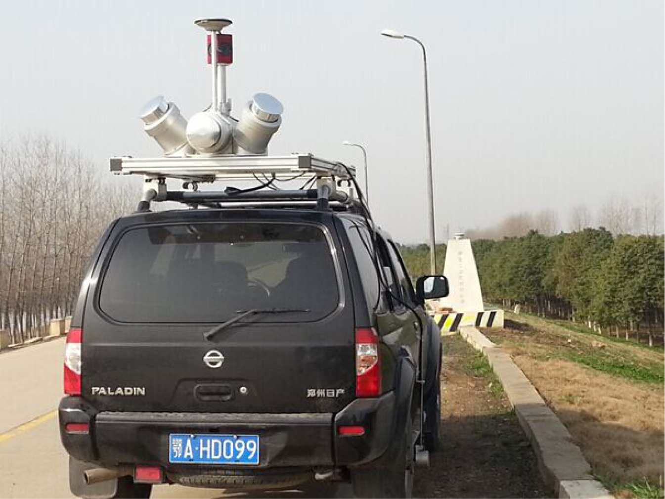
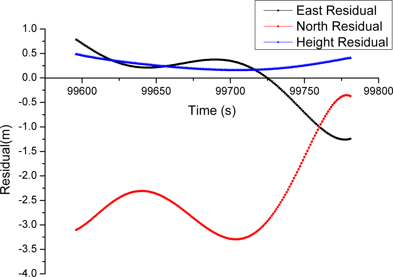
The first experimental trajectory lasted 186 seconds, and 21 control points were laid out along the street section. Figure 4 shows the experimental scenario. For this dataset, we removed the satellites whose elevation angles were smaller than arctan(55°·sin(ψ)), where ψ was the angle difference between the street direction and the satellite azimuth and ranged from 0° to 90°. However, if ψ was smaller than 25°, a satellite would be retained irrespective of its elevation angle. By doing this, we simulated the conditions on an urban street with high buildings or trees. The raw POS trajectory was referred to as the ground truth. The position difference between the simulation results and the ground truth, the residual, at each GNSS epoch was calculated, and the root mean square (RMS), the maximum residual and the minimum residual were computed representing the index of the correction effect. The raw residual at each GNSS epoch is shown in Figure 5, and the coordinate difference of the control points between the LiDAR and the total station measurements is shown in Figure 6.

3.1.1. Comparison between LSC and LS and the Effect of the Order of Polynomials

The LSC correction performance and the least squares (LS) method performance are compared in this part. As mentioned in Section 2.4.1, the LS model only solves the tendency variables, but ignores the random variables. The effect of the polynomial order is also examined. Here, the second-order, the third-order, the fourth-order and the fifth-order polynomials are adopted to fit the tendency variable. All 21 control points are used in this part. δt is set as 30 s.

Table 1. Effect of the polynomial order and comparison between LSC and LS (unit: m).

Method	East			North			Height
	RMS	Min	Max	RMS	Min	Max	RMS	Min	Max
Raw	0.5476	−1.2570	0.7410	2.4528	−3.3000	−0.125	0.2900	0.1520	0.5140
LS-2	0.2009	−0.2868	0.3054	0.4975	−0.8918	0.6479	0.0227	−0.0504	0.0190
LSC-2	0.0576	−0.0723	0.1409	0.1764	−0.4720	0.0656	0.0140	−0.0424	0.0060
LS-3	0.1343	−0.3060	0.2571	0.2964	−0.5496	0.3562	0.0168	−0.0335	0.0114
LSC-3	0.0625	−0.2781	0.0100	0.1469	−0.2848	0.3125	0.0149	−0.0320	0.0073
LS-4	0.0695	−0.0877	0.1440	0.2278	−0.4710	0.1916	0.0171	−0.0334	0.0128
LSC-4	0.0344	−0.0842	0.0959	0.1234	−0.2305	0.0362	0.0142	−0.0311	0.0071
LS-5	0.0392	−0.0551	0.0661	0.1618	−0.3538	0.1381	0.0155	−0.0342	0.0108
LSC-5	0.0278	−0.0391	0.0485	0.1092	−0.2526	0.0422	0.0143	−0.0339	0.0086

C_0E = 0.030 m², C_0N = 0.035 m², C_0H = 0.060 m², δt = 30 s

C_0E = 0.045 m², C_0N = 0.055 m², C_0H = 0.070 m², δt = 30 s

C_0E = 0.045 m², C_0N = 0.070 m², C_0H = 0.080 m², δt = 30 s

C_0E = 0.060 m², C_0N = 0.090 m², C_0H = 0.090 m², δt = 30 s

gives the RMS, the maximum residual and the minimum residual after correction by the LSC and the LS.

As shown in Table 1, the positioning errors with respect to the east, north and height all decrease dramatically after correction either by the LS or LSC. The LS improves the east RMS from 0.5476 m to 0.0392 m, the maximum residual from 0.7410 m to 0.0661 m and the minimum residual from −1.2570 m to −0.0551 m, while the LSC improves them to 0.0278 m, 0.0485 m and −0.0391 m, respectively. The LS improves the north RMS from 2.4528 m to 0.1618 m, the maximum residual from −0.125 m to 0.1381 m and the minimum residual from −3.3000 m to −0.3538 m, while the LSC improves them to 0.1092 m, 0.0422 m and −0.2526 m, respectively. The LS improves the height RMS from 0.2900 m to 0.0155 m, the maximum residual from 0.5140 m to 0.0108 m and the minimum residual from 0.1520 m to −0.0342 m, while the LSC improves them to 0.0143 m, 0.0086 m and −0.0339 m, respectively. These results apparently indicate that the LSC outperforms the LS overall, especially in the east and north. Based on Table 1, we also found that the LSC outstrips the LS more when the polynomial order is lower and that sometimes the performance of a low order LSC equals the performance of a high order LS. This is useful when the number of control points is inadequate for the high order LS fitting.

Generally, the RMS decreases as the order increases, and the maximum and minimum residuals appear to show a similar tendency. However, it should be noted that, for the LSC, a similar Runge phenomenon may appear with an increased order. In fact, this phenomenon is observed in the north and height directions by comparing the performance of the fourth-order LSC and the fifth-order LSC.

Considering that the Runge phenomenon of the fifth-order LSC is not serious and the overall performance of the fifth-order LSC is better than that of the fourth-order LSC, the fifth-order LSC is adopted for further discussion in the following experiments in this subsection.

3.1.2. Effect of the Number of Control Points

In this part, the effect of the number of control points is explored by removing some of them. We reduce the number of control points here from 21 to 15 and 9. The experimental results are shown in

Table 2. Effect of the number of control points (unit: m).

Number	East			North			Height
	RMS	Min	Max	RMS	Min	Max	RMS	Min	Max
Raw	0.5476	−1.2570	0.7410	2.4528	−3.3000	−0.125	0.2900	0.1520	0.5140
21	0.0278	−0.0391	0.0485	0.1092	−0.2526	0.0422	0.0143	−0.0339	0.0086
15	0.0265	−0.0288	0.0440	0.1195	−0.2136	−0.0184	0.0148	−0.0321	0.0147
9	0.0336	−0.0474	0.0677	0.1238	−0.2128	0.0176	0.0160	−0.0403	0.0137

C_0E = 0.060 m², C_0N = 0.090 m², C_0H = 0.090 m², δt = 30 s

C_0E = 0.160 m², C_0N = 0.250 m², C_0H = 0.250 m², δt = 60 s

C_0E = 0.800 m², C_0N = 0.800 m², C_0H = 0.800 m², δt = 120 s

. Here, the correction effectiveness does not decline significantly with a reduced number of control points. Rather, the correction performance using 15 control points is very close to that using 21 and even better on the maximum and minimum residual indexes. This is another similar Runge phenomenon. The correction effectiveness using 9 control points is just a little inferior to that using 15, with a millimetre RMS difference. Fewer control points mean less cost. Thus, when applying a fifth-order LSC for a road section, the recommended number of control points ranges from 9 to 15. However, if the GNSS conditions are extremely poor (for example, if the number of usable GNSS satellites are fewer than 4 at most epochs), the density of control points should be increased. On the other hand, if the GNSS conditions are more favourable (for example, when the number of usable GNSS satellites remains between 4 and 5), the density of control points can be reduced. Mounting a control point on a building unfavourable to GNSS, such as a viaduct, a skyscraper or similar, would also be beneficial.

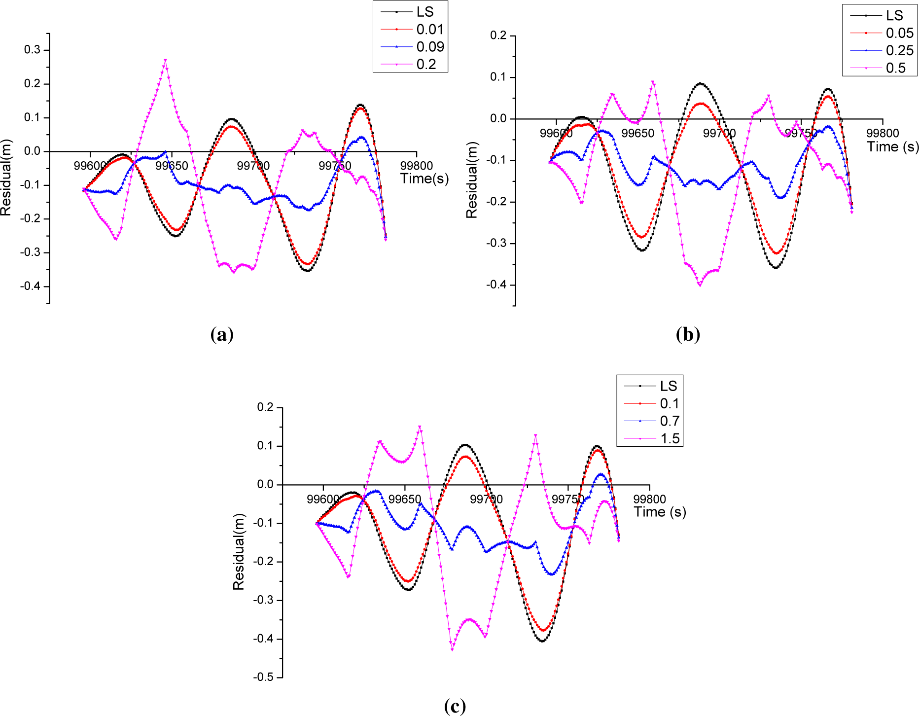
3.1.3. Effect of C₀

C₀ is one of the two key factors determining the value of random variables in the LSC. As C₀ increases, the value of random variables becomes greater. A correct setting for C₀ is therefore of paramount importance. To simplify the discussion, but without becoming too general, we will take the north direction as an example. We will try several values for C₀ for an LSC with 21, 15, 9 control points each and check the RMS. The results of this experiment are given in

Table 3. Effect of C₀.

21	C0(m2)	0.01	0.07	0.08	0.09	0.1	0.11	0.2
	RMS (m)	0.1523	0.1122	0.1099	0.1091	0.1101	0.1125	0.1834
15	C0(m2)	0.05	0.15	0.2	0.25	0.3	0.35	0.5
	RMS (m)	0.1572	0.1304	0.1226	0.1196	0.1217	0.1288	0.1714
9	C0(m2)	0.1	0.5	0.6	0.7	0.8	0.9	1.5
	RMS (m)	0.1679	0.1301	0.1254	0.1233	0.1238	0.1269	0.1856

and shown in Figures 7 and 8a.

The results shown in Table 3 and Figures 7 and 8a are two-fold: firstly, C₀ has an optimal range for each LSC with a different number of control points. Within this range, the random variables are given an appropriate value, and the LSC achieves an optimal performance. If C₀ is set too far below this range, the random variables become too small, and the performance of the LSC will thus be close to that of the LS. Conversely, if C₀ is set too far beyond this range, the random variables become too great, and the LSC will overly correct the positioning error. Secondly, as the number of control points decreases, the optimal value of C₀ and the lower end of the optimal range both increase.

The relationship between the optimal C₀ and the polynomial order is also examined. Figure 8b shows the change in the optimal value of C₀ with the polynomial order. Here, the number of control points is 21. As is clearly shown in Figure 8b, the optimal value of C₀ increases when the order increases. The strict relationship between C₀ and the number of control points, the polynomial order and the conditions affecting the GNSS remains an interesting issue. In practice, we will initialize C₀ with the variance computed by the adopted POS solution software and then adjust it according to its correction performance at check epochs. Thus, for engineering applications, check points are required, as well as control points.

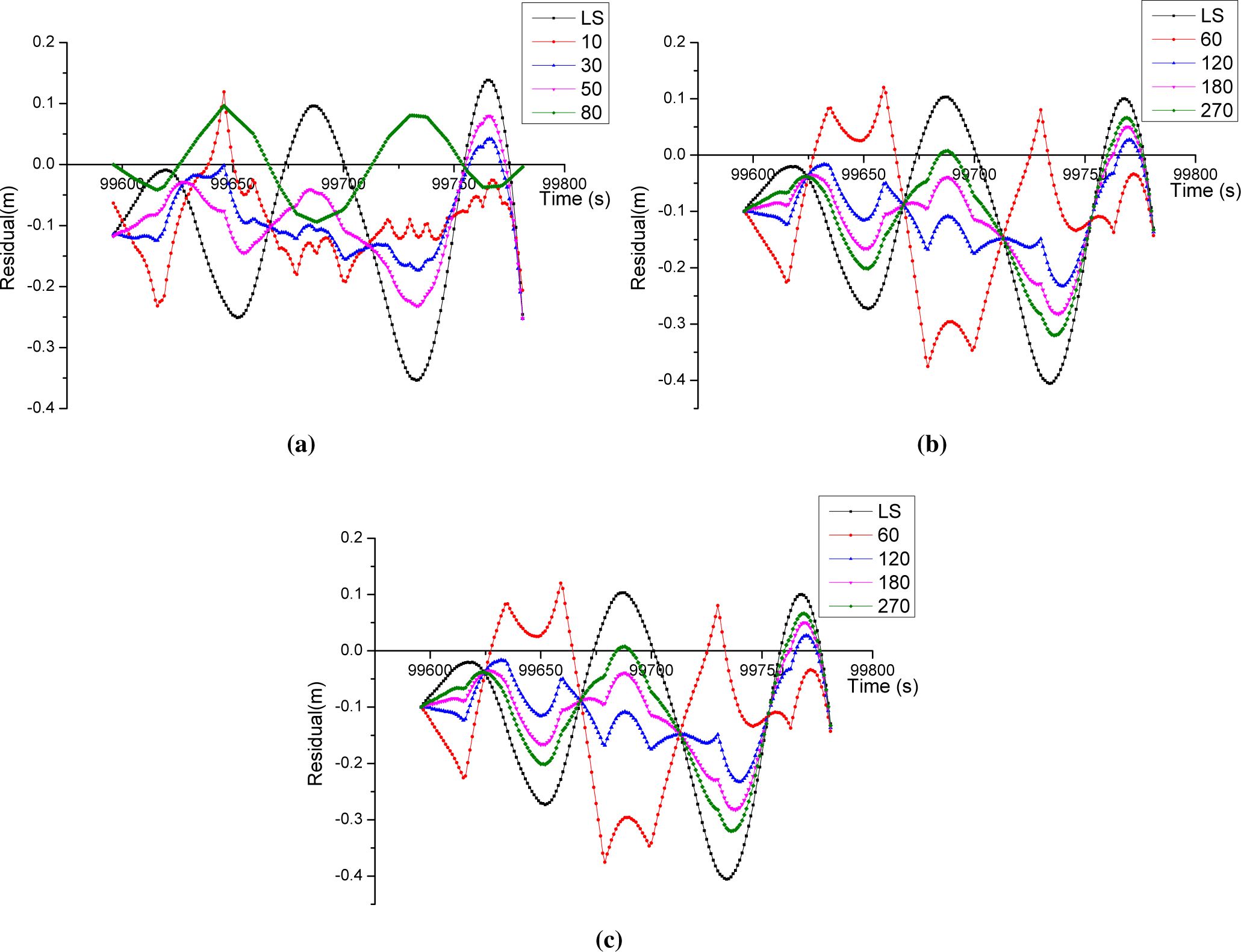
3.1.4. Effect of δt

δt is another key factor affecting the significance of random variables. As far as the LSC with 21, 15 and 9 control points each are concerned, we will test several δt and check the north RMS. The results of the experiment are given in

Table 4. Effect of δt.

21	δt(s)	10	20	30	40	50	80
	RMS (m)	0.1158	0.1122	0.1092	0.1118	0.1163	0.1283
15	δt(s)	20	40	60	80	100	160
	RMS (m)	0.1858	0.1287	0.1196	0.1237	0.1296	0.1429
9	δt(s)	60	90	120	150	180	270
	RMS (m)	0.1654	0.1278	0.1233	0.1269	0.1320	0.1444

and Figure 9.

We find, from looking at Table 4, that δt has an optimal range for each LSC with a different number of control points. The random variables are given an appropriate value within this range, and the LSC achieves optimal performance. However, if δt is set outside this range, the performance of the LSC will decrease. We find from looking at Figure 9 that, except for the impact on the value, δt also affects the temporal smoothness. The bigger the δt, the smoother the change of random variables. According to the results of experiments, the optimal range of δt is 3- to 5-times the average interval between neighbouring control epochs.

3.1.5. Validation Using Boat-Borne Data

Figure 10a shows the second experiment scenario, and Figure 10b shows the points cloud captured from it. This dataset lasted about 151 s. The number of GNSS satellites is kept between 6 and 8 at most epochs. However, since the multipath effect was severe in this dataset, the accuracy of the POS was low, especially in the east and upward directions. There were 9 control points and 15 check points along the river bank. The correction performance of the proposed LSC method and the data-driven method is compared using this dataset. The correction of the data-driven method is carried out through coordinate transformation. The transformation parameters are calculated with control points, and then, the coordinates of the check points are transformed using these parameters. Please note that the horizontal transformation parameters and the height transformation parameters are calculated individually. Figure 11 shows the original coordinate residuals of the check points, as well as those after they have been corrected by the fourth-order LSC and by coordinate transformation.

Table 5. Correction performance of the 4th-order LSC on boat-borne data (unit: m).

Method	East			North			Height
	RMS	Min	Max	RMS	Min	Max	RMS	Min	Max
Raw	0.1071	0.0574	0.1637	0.0264	−0.0629	0.0331	0.2608	0.1742	0.3754
LSC	0.0164	−0.0258	0.0460	0.0213	−0.0512	0.0382	0.0422	−0.0514	0.0882
Transformation	0.0310	−0.0644	0.0431	0.0256	−0.0529	0.0417	0.0616	−0.0818	0.1195

C_0E = 0.400 m²,C_0N = 0.010 m²,C_0H = 0.800 m², δt = 120 s

gives the RMS and the maximum and minimum residuals. As is shown in Table 5 and Figure 11, the accuracy with respect to the east and the height have been significantly improved both by the fourth-order LSC and by coordinate transformation. The fourth-order LSC improves the east RMS from 0.0574 m to 0.0164 m, the north RMS from 0.0264 m to 0.0213 m and the height RMS from 0.2608 m to 0.0382, respectively, while the coordinate transformation method improves them to 0.0310, 0.0256, 0.0616, respectively. In this scenario, the proposed method apparently outperforms the coordinate transformation method.

3.2. Validation for the LSC-Based Calibration Method

The proposed LSC-based calibration method is validated in this section. The initial translations and rotations were set to (−0.0192, 0.0142, 0.3619) m and (0, 0, 180)°, respectively. Ten control points were adopted for misalignment calibration, and the other 54 points were used as check points.

Table 6. Misalignment calibrated by the proposed LSC model and the LS method.

Method	ΔTx (m)	ΔTy (m)	ΔTz (m)	Δθx (Degree)	Δθy (Degree)	Δθz (Degree)
LS	0.0005	0.0145	−0.0645	−0.0307	−0.0550	0.2077
LSC	0.0004	0.0145	−0.0642	−0.0307	−0.0561	0.2077

gives the calibration results calculated by the proposed LSC method and the LS method. The RMS of the coordinates at the check points are given in

Table 7. RMS of the coordinates of check points.

Method	East	North	Height
Raw	0.0775	0.0544	0.0909
LS	0.0256	0.0227	0.0303
LSC	0.0141	0.0114	0.0233

C_0E = C_0N = C_0H = 0.0004 m², δt = 120 s

, and the residuals are shown in Figure 12.

As Table 6 would indicate, the misalignments calibrated by the LSC method and the LS method are almost equal to each other. However, as is shown in Table 7 and Figure 12, the RMS of the check point coordinates calculated by the LSC method is smaller than that calculated by the LS method, with the residuals being closer to zero. The reason why the RMS and residuals calculated by the LSC are better than those calculated by the LS is that the LSC eliminates both the random positioning and orientation errors. Therefore, although the LSC calibration method achieved a similar result to the correction of misalignment by using the LS method, the LSC method is, in fact, more suited to an accuracy evaluation of misalignment calibration.

4. Conclusions

In this paper, an LSC method was proposed to improve the accuracy of MLS. In environments hostile to GNSS, the POS error became the main error source of MLS. According to theoretical analysis, the POS error consisted of a tendency part and a random part. The tendency part of the POS error was modelled by a polynomial varying with time, and the random part satisfied a zero-mean distribution. As a result, the correction parameters of the POS error could be solved by the LSC methods. Experiments on the simulated datasets showed that the fifth-order LSC improved the east RMS of the POS error from 0.5476 m to 0.0278 m, the north RMS from 2.4528 m to 0.1092 m and the height RMS from 0.2900 m to 0.0143 m, while the LS method improved them to 0.0392 m, 0.1618 m and 0.0155 m, respectively. These results clearly indicated that the LSC method made a much more effective improvement for POS accuracy than the traditional LS method. The effect of the polynomial order, the number of control points, the correlation time δt and basic covariance value C₀ were also discussed in detail. Generally, the performance of LSC became better when the polynomial order increased. The fourth-order and the fifth-order LSC were recommended for engineering applications. When the number of control points was decreased from 21 to 15 and 9, the performance of the LSC method did not show significant decrease. Fewer control points mean less cost. When applying a fifth-order LSC for a road section, the recommended number of control points ranges from nine to 15, depending on the environment. C₀ and δt were the two key factors determining the value of random variables in the LSC. We found that δt had an optimal range varying with the number of control points, and C₀ also had an optimal range varying with the polynomial order, as well as the number of control points. Furthermore, experiments on a real vehicle-borne dataset, which suffered from a severe multi-path effect, indicated that the proposed LSC method outperformed the traditional coordinate transformation method.

The proposed LSC method was also applied to calibration of the misalignment between the laser scanner and the POS, in which the misalignment parameters were treated as tendency variables, and the positioning error and the orientation error were both treated as random variables. Experimental results on the real dataset showed that the LSC-based calibration method obtained a calibration precision more accurate than the traditional LS method, though they got similar misalignment parameters.

In summary, the proposed LSC method represented an effective improvement for MLS accuracy. It can be widely applied in MLS surveying engineering, such as virtual 3D city reconstruction, highway surveying, rail road surveying, mine surveying, and so on, which will keep the high accuracy of points cloud data in harsh GNSS conditions.