Article

Spatial Variability Mapping of Crop Residue Using Hyperion (EO-1) Hyperspectral Data

by
Abderrazak Bannari
1,*,
Karl Staenz
2,
Catherine Champagne
3 and
K. Shahid Khurshid
4
1
GeoInformatics Department, Arabian Gulf University, P.O. Box 26671, Manama, Kingdom of Bahrain
2
Alberta Terrestrial Imaging Centre (ATIC), Department of Geography, University of Lethbridge, 401, 817 4th Avenue South, Lethbridge, AB T1J 0P, Canada
3
Agriculture and Agri-Food Canada, 960 Carling Avenue, Ottawa, ON K1A 0C6, Canada
4
Earth Observation and Geomatics, Meteorological Service of Canada, Environment Canada, 373 Sussex Drive, Ottawa, ON K1A 0H3, Canada
*
Author to whom correspondence should be addressed.
Remote Sens. 2015, 7(6), 8107-8127; https://0-doi-org.brum.beds.ac.uk/10.3390/rs70608107
Submission received: 12 April 2015 / Revised: 10 June 2015 / Accepted: 15 June 2015 / Published: 18 June 2015

Abstract

:
Soil management practices that maintain crop residue cover and reduce tillage improve soil structure, increase organic matter content in the soil, positively influence water infiltration, evaporation and soil temperature, and play an important role in fixing CO2 in the soil. Consequently, good residue management practices on agricultural land have many positive impacts on soil quality, crop production quality and decrease the rate of soil erosion. Several studies have been undertaken to develop and test methods to derive information on crop residue cover and soil tillage using empirical and semi-empirical methods in combination with remote sensing data. However, these methods are generally not sufficiently rigorous and accurate for characterizing the spatial variability of crop residue cover in agricultural fields. The goal of this research is to investigate the potential of hyperspectral Hyperion (Earth Observing-1, EO-1) data and constrained linear spectral mixture analysis (CLSMA) for percent crop residue cover estimation and mapping. Hyperion data were acquired together with ground-reference measurements for validation purposes at the beginning of the agricultural season (prior to spring crop planting) in Saskatchewan (Canada). At this time, only bare soil and crop residue were present with no crop cover development. In order to extract the crop residue fraction, the images were preprocessed, and then unmixed considering the entire spectral range (427 nm–2355 nm) and the pure spectra (endmember). The results showed that the correlation between ground-reference measurements and extracted fractions from the Hyperion data using CLMSA showed that the model was overall a very good predictor for crop residue percent cover (index of agreement (D) of 0.94, coefficient of determination (R2) of 0.73 and root mean square error (RMSE) of 8.7%) and soil percent cover (D of 0.91, R2 of 0.68 and RMSE of 10.3%). This performance of Hyperion is mainly due to the spectral band characteristics, especially the availability of contiguous narrow bands in the short-wave infrared (SWIR) region, which is sensitive to the residue (lignin and cellulose absorption features).

Graphical Abstract

1. Introduction

Conservation of post-harvest crop residue on agricultural land plays an important role in the protection of the soil surface against water and wind erosion [1,2,3]. Regarding the environmental benefits [4], crop residue improves soil structure, increases organic matter content in the soil, positively influences water infiltration, evaporation and soil temperature [5], and plays an important role in fixing CO2 in the soil [6]. Consequently, good residue management practices on agricultural land have many positive impacts on soil quality and crop production. In the literature, several spectral indices for quantitative evaluation of the crop residue cover have been developed [4,7,8,9,10,11,12,13]. Although the initial demonstration of these techniques was successful, application of empirical models are in general difficult to be applied to other locations with different conditions. Even though the relationship between the parameter in question and specific index can be re-established to address these differences, it is no guarantee that a satisfactory relationship can be found [9,10]. Accordingly, these methods are not sufficiently rigorous and accurate for discriminating residue from bare soil and for estimating the fraction of residue cover [14]. They do not consider the spectral mixture of different materials in the same pixel [15,16]. Moreover, the broad spectral and spatial resolutions of multispectral sensors do not allow an accurate analysis of the composition of the target materials on the ground [17]. Using hyperspectral (Probe-1) data and the constrained linear spectral mixture analysis (CLSMA) approach, the estimation of percent crop residue cover was improved but was not accurate enough, because the image data were acquired when the crop vigor was very developed and very high [18]. Accordingly, the crop residue was shaded and/or completely covered, and therefore, the performance of the proposed approach was reduced. Acquisition of imagery post-harvest or prior to spring seeding would simplify the extraction of percent residue cover by eliminating confusion with the crop canopy.
Monitoring agricultural land from space has been restricted in the past by low temporal, spatial and spectral resolution. The evolution of information technologies and a better understanding of the interactions between electromagnetic radiation and different terrestrial targets have opened up new potential for remote sensing applications. The management and planning of natural resources and the environment make satellite and airborne remote sensing one of the key technological tools for this century. Imaging spectroscopy, or more commonly hyperspectral remote sensing, has emerged as a new technology in optical remote sensing for the management of natural resources and the environment [19]. Numerous airborne and a few satellite hyperspectral sensors have been developed to survey the Earth’s surface and retrieve quantitative information for various applications, such as agriculture, forestry, geology, mineralogy, hydrology and oceanography [20,21,22,23].
Hyperspectral remote sensing allows the simultaneous acquisition of images in hundreds of narrow contiguous bands in specific regions of the electromagnetic spectrum [20,24,25]. The spectral resolution of this technology is very close to that achieved in laboratories and field measurements, thus, enhancing the ability to identify materials on the Earth’s surface from aircraft or spacecraft platforms. The reflectance spectrum in the 400 nm–2500 nm region can be utilized to distinguish a large variety of surface cover materials, which is not possible with broadband sensor technology [26]. Comparing hyperspectral Probe-1 and multispectral high-spatial resolution IKONOS data with a similar spatial resolution, Bannari et al. [18] have demonstrated the potential of hyperspectral imaging for crop residue mapping. Using the Landsat Thematic Mapper (TM), Airborne Visible Infrared Imaging Spectrometer (AVIRIS) and Hyperion Earth Observing-1 (EO-1) imagery, acquired prior to spring crop planting, Daughtry et al. [2,17] showed that the spectral crop residue indices using TM bands were weakly related to crop residue cover, whereas the AVRIS and Hyperion data were relatively accurate in estimating the percentage of crop residue cover.
The advent of hyperspectral remote sensing not only requires new technology for instruments, but also new analytical approaches and techniques to manipulate and process data and extract information from hundreds of spectral bands at a time [20,26,27,28,29]. Several new techniques have been developed to analyze hyperspectral data, including linear spectral mixture analysis [30,31,32,33,34,35]. It assumes that the source of the spectral signature from a pixel is produced by more than one spectrally distinct component. The fundamental assumption of this technique is that generally each pixel is a physical mixture of several constituents weighted by the surface abundance, while the spectrum of the mixture is a linear combination of the endmember reflectance spectra which represent the pure target materials.
The objective of this study was to investigate the potential of the Hyperion (EO-1) hyperspectral data and CLSMA for estimation and mapping of fractional crop residue cover, using ground data for validation purposes.

2. Material and Methods
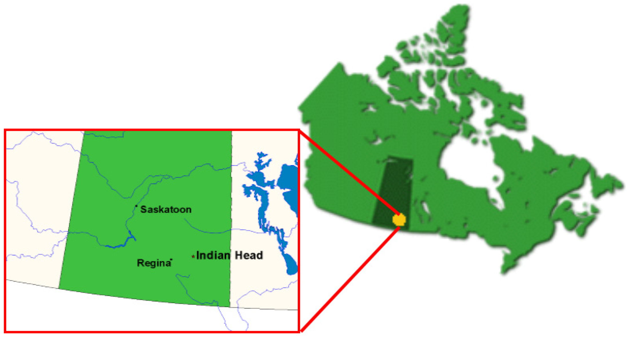
2.1. Study Site

The data were collected in an agricultural region near Indian Head (50°N, 104°W), approximately 70 km east of Regina, Saskatchewan, Canada (Figure 1). The selected site is an intensively cultivated agricultural area dominated by black Chernozemic soils, which developed on neutral to slightly alkaline and uniform clayey lacustrine deposits. The climate can be regarded as typical northern continental. Hot temperatures and occasional dry periods characterize the summer. The winter is cold and snowy with temperatures remaining below freezing until early March. The principal economic activities of this area are based on agricultural practices. Generally, the major crops grown are wheat (Triticum aestivum L.), pea (Lathyrus aphaca L.), canola (Brassica napus L.), and corn (Zea mais L.). The most dominant crop was wheat followed by pea and canola. The test fields are located around the Indian Head Agricultural Research Foundation (IHARF) experimental farm. Ground and image data were acquired before the beginning of the agricultural season with no tillage and seeding applied to the fields. Therefore, no crop (or weeds) emerged from the soil (Figure 2). For validation purposes, sampling points of different wheat residue cover were selected in 10 fields of various sizes (0.7 to 8 km2). These points were distributed randomly throughout the study area. Within these fields, a total of 77 sampling points with different residue densities were selected with 6 to 8 sampling points per field.
Figure 1. Study site, Indian Head, Saskatchewan (Canada).
Remotesensing 07 08107 g001
Figure 2. True-color composite of the Hyperion 3D cube sub-scene (7.50 km by 16.08 km) and acquired photographs of residue (a,b), soil status (c), and mixed soil and residue (d) for validation purposes.
Remotesensing 07 08107 g002

2.2. Image Data Acquisition

Image data were acquired on 20 May 2002 using the Hyperion hyperspectral sensor on NASA’s Earth Observer-1 (EO-1) platform (Figure 2). This sensor collects the upwelling radiance in 242 spectral bands, each 10 nm wide with an average spectral sampling interval of 10 nm [36]. It has a single telescope and consists of two spectrographs, one covering the visible and near-infrared (VNIR) wavelength range from 357 nm to 1055 nm, and the other covering the short-wave infrared (SWIR) from 851 nm to 2576 nm. Its telescope images the Earth onto a slit with a field-of-view (FOV) of 0.624°, resulting in a ground sampling distance (GSD) of 30 m, and a swath width of 7.65 km from a 705 km altitude [37]. The size of the sub-scene used in this research (region of interest) covers an area of 7.50 km (254 pixels) by 16.08 km (536 lines).

2.3. Image Data Pre-Processing

2.3.1. Radiometric and Spectral Calibration

The Hyperion data were pre-processed with an objective to correct for sensor artifacts and atmospheric and geometric effects [38]. The Imaging Spectrometer Data Analysis System (ISDAS) developed at the Canada Centre for Remote Sensing [28] but accessible to Canadian remote sensing scientists, was used to perform all the pre-processing steps. A flowchart shown in Figure 3 summarizes all pre-processing steps. The procedure begins with geometric corrections (shift and rotation) of the SWIR data to spatially register them with the VNIR data. Furthermore, the striping problem due to systematic noise caused by factors, such as detector non-linearity, movement of the slit with respect to the focal plane and temperature effects, was corrected [39]. In addition, the column dropouts caused by dead pixels (a dead pixel is a functional failure of a single detector element during acquisition) were then removed from the whole image cube [40]. This was followed by noise reduction using automated software in the ISDAS system [38]. To achieve this step, the raw imagery (digital numbers) recorded by the sensor was converted to at-sensor radiance using the radiometric calibration coefficients (gains and offsets) derived in the laboratory and provided by NASA [41].
The data cube was subsequently analyzed to characterize the distortions of keystone and spectral smile [42]. At this step, the data were cropped to exclude noisy bands resulting in a final data set that spans the spectral range from 427 nm to 2355 nm with a total of 192 bands (excluding the overlap bands between the VNIR and SWIR spectrographs). Keystone is a term used in hyperspectral remote sensing to refer to the inter-band spatial mis-registration in imaging spectrometers [43]. These distortions may be caused by geometric distortions or by chromatic aberration, or a combination of both. Due to these distortions, a particular spatial pixel, corresponding to a specific detector element in the across-track dimension in one specific band will not be registered on the ground with the corresponding pixel in the other spectral bands. Neville et al. [43] reported that the Hyperion sensor has minor keystone distortions, ranging from −0.05 to 0.49 pixels for the VNIR spectrometer and −0.06 to 0.07 pixels for the SWIR spectrometer. For our data, the keystone distortion was not significant, i.e., from a minimum of −0.075 pixels to a maximum of 0.3 pixels for the VNIR and 0.1 pixels for the SWIR [38]. Accordingly, no keystone correction was performed.
Furthermore, the spectral smile/frown is a wavelength shift, which is a function of the across-track pixel (column) in the swath [44]. In an ideal case, all pixels in the across-track dimension correspond to the same wavelength. This wavelength shift is due to many sources, such as spatial distortions caused by the dispersion element, prism or grating, or by aberrations in the collimator and imaging optics [42]. To achieve spectral calibration, the at-sensor radiance spectra were analyzed to evaluate the bandwidth and band’s center position using five known atmospheric absorption features: 760 nm (oxygen), 940 nm and 1130 nm (water vapor) and 2005 nm and 2055 nm (carbon dioxide). The correct band-center wavelengths and bandwidths are determined by correlating the at-sensor Hyperion radiance with a modeled at-sensor radiance calculated with the radiative transfer (RT) code MODTRAN 4.2 [45]. Wavelength shifts of 1–3 nm were observed in the VNIR and SWIR and applied after the atmospheric correction process.
Figure 3. Hyperspectral data (Hyperion EO-1) pre-processing steps for retrieval of surface reflectance data.
Remotesensing 07 08107 g003

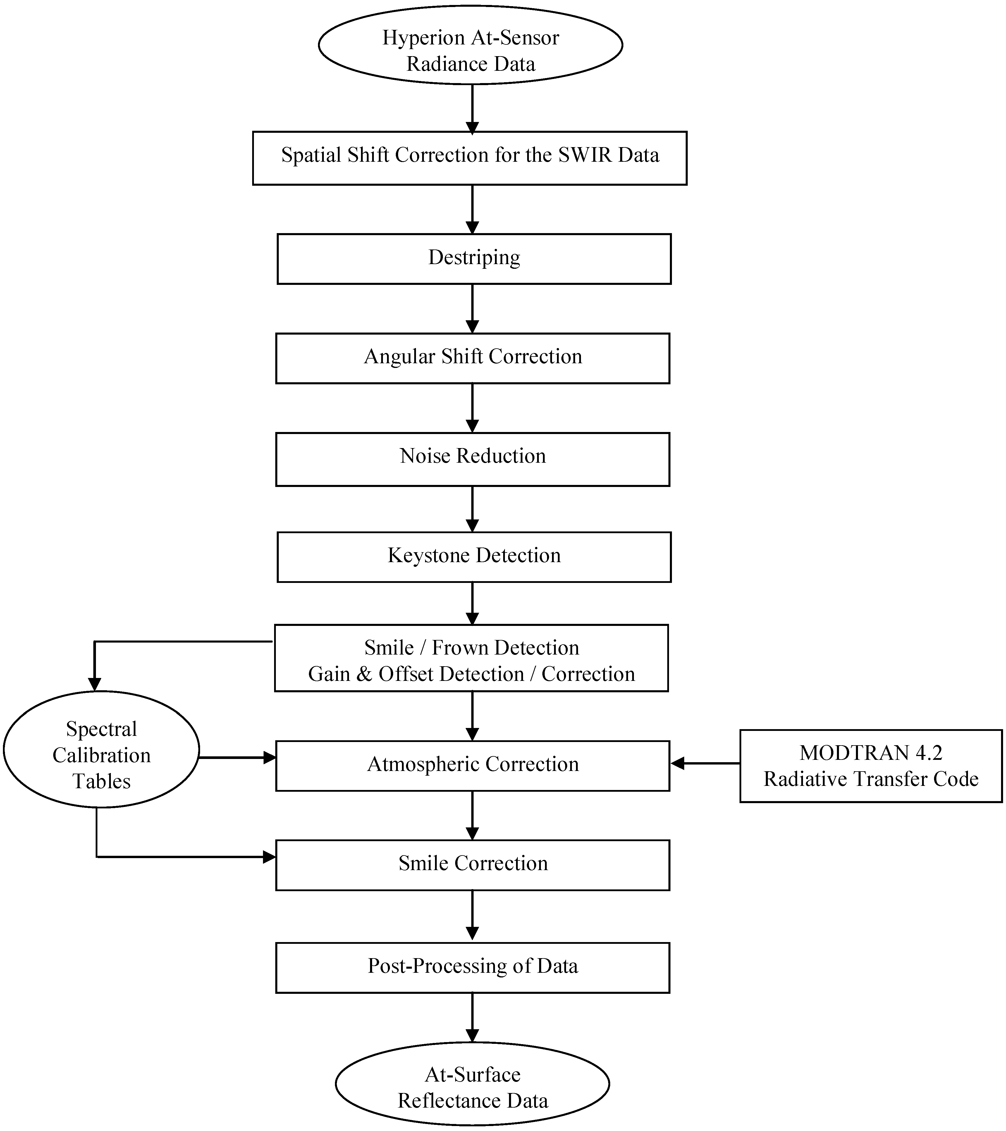
2.3.2. Surface Reflectance Retrieval

The calibrated at-sensor radiance data were converted to surface reflectance using a look-up table (LUT) approach to correct for the atmosphere [46]. Two five-dimensional raw LUTs, each one for a 5% and 60% spectrally flat reflectance, with tunable breakpoints were generated with the selected RT code to provide additive and multiplicative coefficients for the removal of atmospheric scattering and absorption effects. The MODTRAN-4.2 RT code was applied to the imagery using a midlatitude–summer atmosphere model and a continental–rural aerosol model. The input parameters for the RT code are presented in Table 1. The LUTs were convolved with the Hyperion sensor characteristics and then used in combination with a curve-fitting technique in the 940 nm and 1130 nm water vapor absorption regions to estimate the atmospheric water vapor content from the image data on a pixel-by-pixel basis [47,48]. The column atmospheric water vapor estimates were then interpolated using the LUTs to retrieve surface reflectance. Subsequently, the reflectance data were corrected for smile effects.
Table 1. Input parameters for the MODTRAN 4.2 radiative transfer code.
Date of over flight20 May 2002
Time of over flight (GMT)17:42:36
Solar zenith angle33.3536°
Solar azimuth angle149.7354°
Atmospheric modelMid-latitude summer
Aerosol modelContinental (rural)
Terrain elevation (ASL)0.579 km
Horizontal visibility23 km
Water vapour1.5–2.5 mg/cm2
CO2 mixing ratio365 ppm (as per model)
GMT = Greenwich Mean Time; ASL = Above Sea Level; ppm = parts per million.
Finally, the post-processing concluded the corrections by removing residuals that still remained after the correction of sensor artifacts and atmospheric effects. This step involved the calculation of correction gains and offsets using a spectrally flat target pixel approach [49]. The technique assumes that there are a number of pixels whose reflectance spectra are flat, or nearly flat (feature-less), and their brightness range covers a major portion of the full range for all the pixels in the scene. A second-order polynomial fit to the reflectance spectra using χ-squared as a goodness of fit measure is calculated on a pixel-by-pixel basis. The pixels with the smallest χ-squared values are selected as “spectrally flat target pixels”. Finally, linear fits are performed on a band-by-band basis providing slopes and offsets, which are used as gain and offset for the correction of residual errors in the reflectance data.

2.3.3. Image Geo-Referencing

In order to preserve the radiometric integrity of each image pixel, the Hyperion data were resampled only when the SWIR was registered to the VNIR. Champagne [50] reported a technique that locates sampling points in the hyperspectral image (master) by first locating them on a geo-referenced image (slave) and then warping this image to match the hyperspectral data. For this purpose, a high-spatial resolution (0.69 m) panchromatic QuickBird image of the study area was used to locate the sampling plots for validation purposes. The locations of these were measured during ground-data acquisition with a differential global positioning system (DGPS) assuring less than ±1 m accuracy. The locations of the sampling plots were “burned” (encoding vector information into a raster image) into the QuickBird image using PCI Software [51] so that the locations would still be detectable in the warped image. The QuickBird image was then registered to the Hyperion imagery with a 2nd order polynomial. About 20 ground control points (GCPs) were selected at the corner of each field and intersections of roads from both images. The GCPs were selected evenly over the entire image to get a better image fit and even the distribution of registration errors. In the registration process, a cubic convolution resampling method was used. This approach applies the weighted average of the 16 surrounding pixels (i.e., 4 pixel × 4 pixel window) to calculate the reflectance. Finally, pixel and line coordinates from the warped image were recorded for each sampling point. For the registration accuracy between QuickBird and Hyperion data, the root mean square error (RMSE) was 0.33 and 0.61 pixel in x and y directions, respectively. Finally, the recorded pixel and line coordinates of each sampling plot were used to extract information (from Hyperion data), which was carried out using the information extraction network in ISDAS.

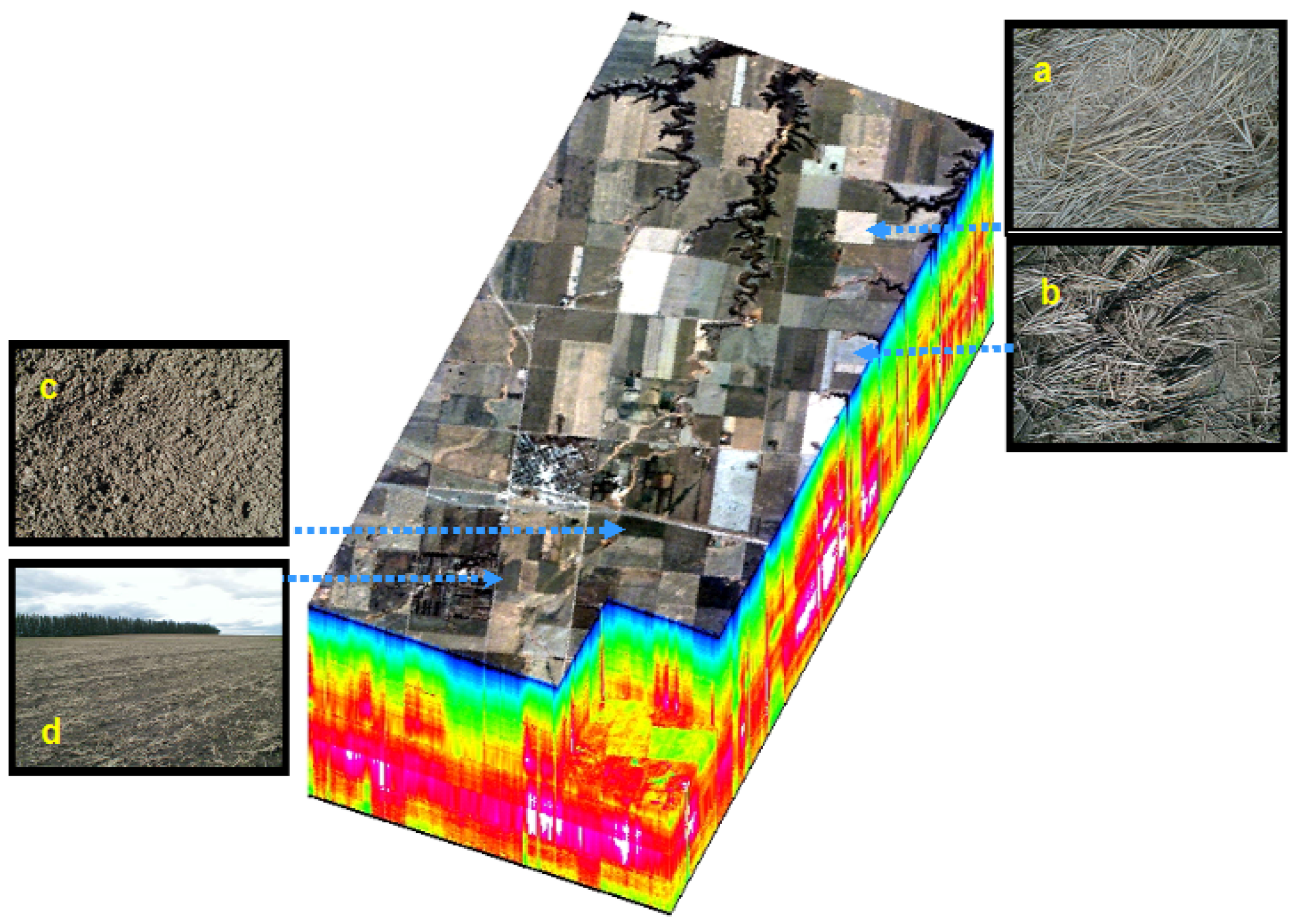
2.4. Ground-Data Acquisition

Ground spectroradiometric measurements were collected simultaneously with the Hyperion data acquisition (20 May 2002) in two fields, considering four different targets: dry and slightly moist wheat residue, and dry and a slightly moist dark soil. The relatively low number of samples is due to the fact that pure residue targets are extremely hard to find, because they are generally mixed with soil. The same is true for pure soil targets. The selected targets were acquired using a GER-3700 spectroradiometer [52] over naturally occurring dense patches of residue and bare soil to reflect the same moist and dryer conditions as the Hyperion data. The GER-3700 instrument measures radiance over a spectral range from 400 nm to 2500 nm using 704 spectral bands varying from 1.5 nm to 20 nm at full-width half-maximum (FWHM). The 10° FOV of the GER 3700 was used and the distance between the target and the instrument was 1.85 m, which provided a diameter of 32.37 cm on the ground. Surface reflectance was calculated by ratioing target radiance to the radiance obtained from a calibrated 25 cm by 25 cm white Spectralon panel [54], according to the method described by Jackson et al. [55]. Corrections were made for the wavelength dependence and non-Lmbertien behavior of the panel. The Spectralon radiance was acquired immediately before the target radiance. For each considered target material, the average of 20 spectra from pure patches in different fields was calculated using the GER-3700. The averaged spectra were then convolved with the Gaussian response profiles in ISDAS to match the bandwidths and the band centers of the Hyperion EO-1 sensor.
For validation purposes, ground-percent crop residue cover was calculated from vertical photographs taken at each sampling plot and compared to extracted results from CLSMA. These photographs were taken with a 35 mm camera equipped with a 28 mm lens. The camera was mounted on an overhead mast and used at a height of 2 m above ground. In this configuration, the camera viewed a ground area of about 5 m2. Given that the Hyperion data have a pixel size of 30 × 30 m2, five photographs were acquired within 3 m to 6 m of the center of the sampling site locations (depending on the density of the residue) for greater site representation. The perspective center of each photo was localized using the DGPS.

2.5. Image Processing

2.5.1. Ground-Photo Classification

The vertical ground digital photographs acquired in three channels (blue, green and red) were classified using an unsupervised ISODATA classifier in PCI Image Works [51]. This step was carried out using the following five classes: soil, dry residue, moist residue, shaded residue, and shaded soil. These classes were then automatically aggregated into two major components: residue and soil. Based on this decision, and on the photos’ histogram analysis [44,53], all pixels were classified. When there are only two or three classes this method is the most popular and the most used for validation purposes in the remote sensing field [14,15,16,56,57]. A visual inspection with the ground photographs confirmed the obtained results from the unsupervised classification. Once the classification was completed, percentages of soil and residue cover were determined for each photograph by dividing the number of pixels for each component with the total number of pixels in the photograph. Final percent crop residue cover was then calculated from the average of the five replicate photographs per sampling plot and compared to the extracted fractions of soil and residue for the 77 sites in the 10 fields. All these fields were only representing residue of wheat.

2.5.2. Constrained Linear Spectral Mixture Analysis (CLMSA)

Linear spectral mixture analysis (LSMA) approaches have been used extensively in geology, soil, land use, forestry and agriculture applications [18,29,50,58,59,60,61,62]. This method assumes that the source of the spectral signature from a pixel is produced by more than one spectrally distinct component [58]. The fundamental assumption of LSMA is that generally each pixel on the surface is a physical mixture of several constituents weighted by the surface abundance, and the spectrum of the mixture is a linear combination of the endmember reflectance spectra. In spite of the omission of the multiple scattering effects among different targets in the pixel, the errors associated with the linear assumptions have been found insignificant [63,64]. The general equation that expresses LSMA is as follows [31,65]:
R b   = i = 1 m f i r b i + e b
where
         i = 1 m f i = 1.0 ,       0     f i   1
Rb is the reflectance of a pixel in band b, fi is the fractional abundance of endmember i, m is the total number of endmembers, rbi is the reflectance in band b of endmember i, and eb is the residual error in band b of the model. Equation (2) represents the CLSMA case compared to the unconstrained linear spectral mixture analysis, where the sum of the fractions can be larger than 1 and the individual fractions can be lower and/or higher than 1 [61]. CLSMA was performed on Hyperion imagery using an algorithm implemented in ISDAS [31,66] and was carried out using the full spectral range from 428 nm to 2355 nm. As a result, the crop residue fraction map was derived from the Hyperion data for each individual field. The values range from 0 to 1, where 0 indicates a very low abundance and 1 a high abundance. Finally, the percent crop residue cover (PCRC) and the percent soil cover (PSC) were validated with the ground vertical photographs taken during the field campaign.

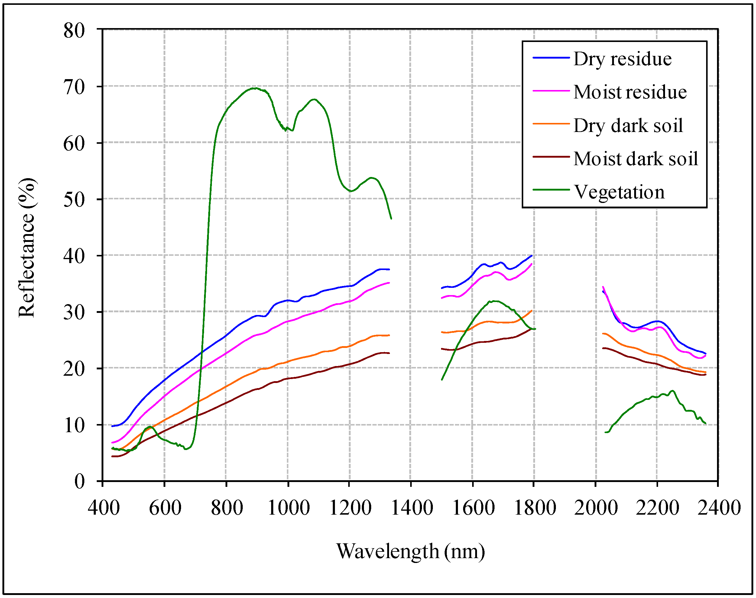
2.5.3. Endmember Measurement

Endmember selection is the most important step to successfully unmix the reflectance data cube and produce valid fractional abundances for the study site. Improper endmember selection and identification can lead to meaningless percent (fraction) cover maps, especially if the endmember spectra are inaccurate in a physical sense [32]. In order to minimize the sources of errors and to increase the accuracy of crop-residue estimation, image data were acquired at the beginning of the agricultural season [18]. In this period, primarily only bare soil and crop residue (only a few centimeters in height) are present and no crop development have started yet (Figure 2). However, a vegetation endmember was considered from our spectral library, which has been generated from the site under study over several years. This endmember was adequate to represent the coniferous trees (Figure 2d) and all other photosynthetically targets in the scene. The other endmembers were collected in the field, simultaneously with Hyperion data acquisition, using a GER-3700 spectroradiometer as described in Section 2.4. These endmembers were measured from natural “pure” patches (Figure 2a,b), which were considered representative of the wheat residue and bare soil in the study site (Figure 2c,d). Other residue types such as pea, canola and corn were also present in the study area, but they could not be measured due to their sparse distribution and degraded appearance. Accordingly, only the dry and slightly moist wheat residue and soil were used together with the vegetation endmember in the CLSMA. The resulting fractions of both residue components were added to form one fraction map of residues. The same was done for soil. It is important to mention that a crop residue shadow endmember was not included given that the study area is very flat, crop cover was absent, and crop residue was only few centimeters in height (Figure 2a,b). Consequently, basically no shadow component existed in the considered fields (sun elevation and azimuth were 56.65° and 149.73°, respectively). Scene-based endmembers were not considered due to the Hyperion 30 m GSD and the relatively small patches of homogeneous residue cover, which would have led to endmembers not representing pure residue.

2.6. Statistical Analyses

Statistical analyses were computed with the Statistica software [67]. Various statistics were computed for both ground measurements (observed values) and image data (predicted values). Standard deviation statistics allowed the evaluation of data variability. This parameter was reported in all cases as an error percentage of the average extracted from ground measurements (vertical photographs) and image data. To validate PCRC and PSC, ground measurements and image data were compared using the 1:1 line. Ideally, observed and predicted values should have a correspondence of 1:1. The index of agreement, D, reflects the degree to which the observed value is accurately estimated by the predicted value. This measure was calculated as follows [68]:
D = 1 [ i = 1 n ( P i O i ) 2 i = 1 n ( | P i | + | O i | ) 2 ]
where Pi is the predicted value at sample i, Oi is the observed value at sample i, Pi′ is the difference between Pi and the average of the predicted values, and Oi′ is the difference between Oi and the average of the observed values and n is the number of values. This index provides a measure of the degree to which a model’s predictions are error free. The index ranges between 0 and 1, with 1 indicating a perfect match between observed and predicted values. The observed values were those calculated from the vertical photographs and the predicted values were from the abundance maps. The RMSE was used as an overall error to supplement the index of agreement described above. This error also quantifies the 1:1 relationship between observed and predicted values. It was calculated as follows [68]:
  R M S E   =   i = 1 n ( P i O i ) 2 n  
The relationships between observed and predicted values were also analyzed using a linear regression model. The coefficient of determination (R2) of the regression model was also used to evaluate the strength of the linear relationship between observed and predicted values.

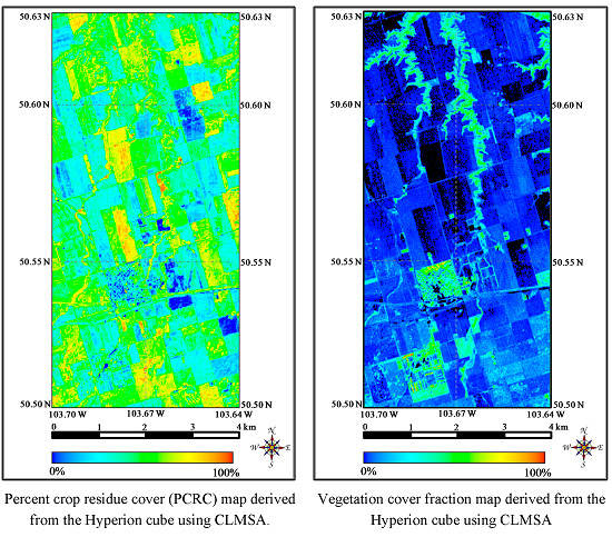
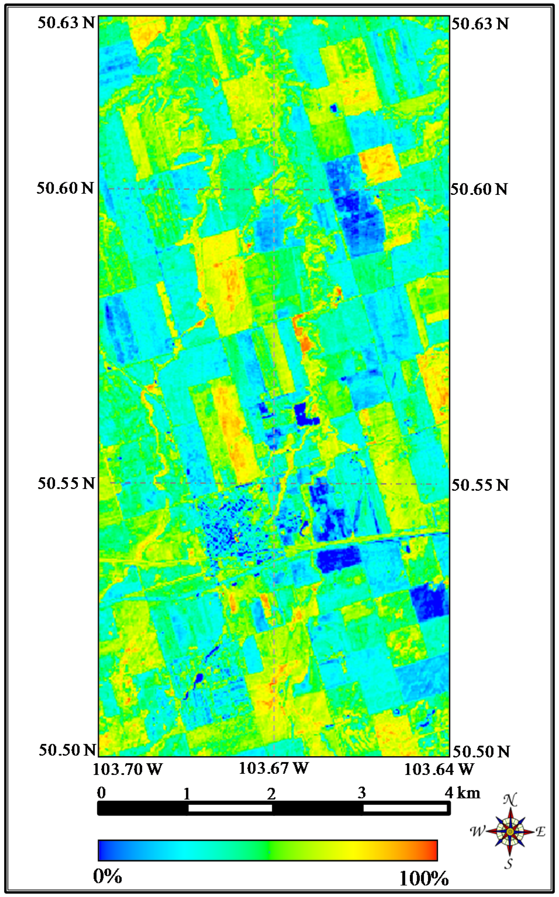
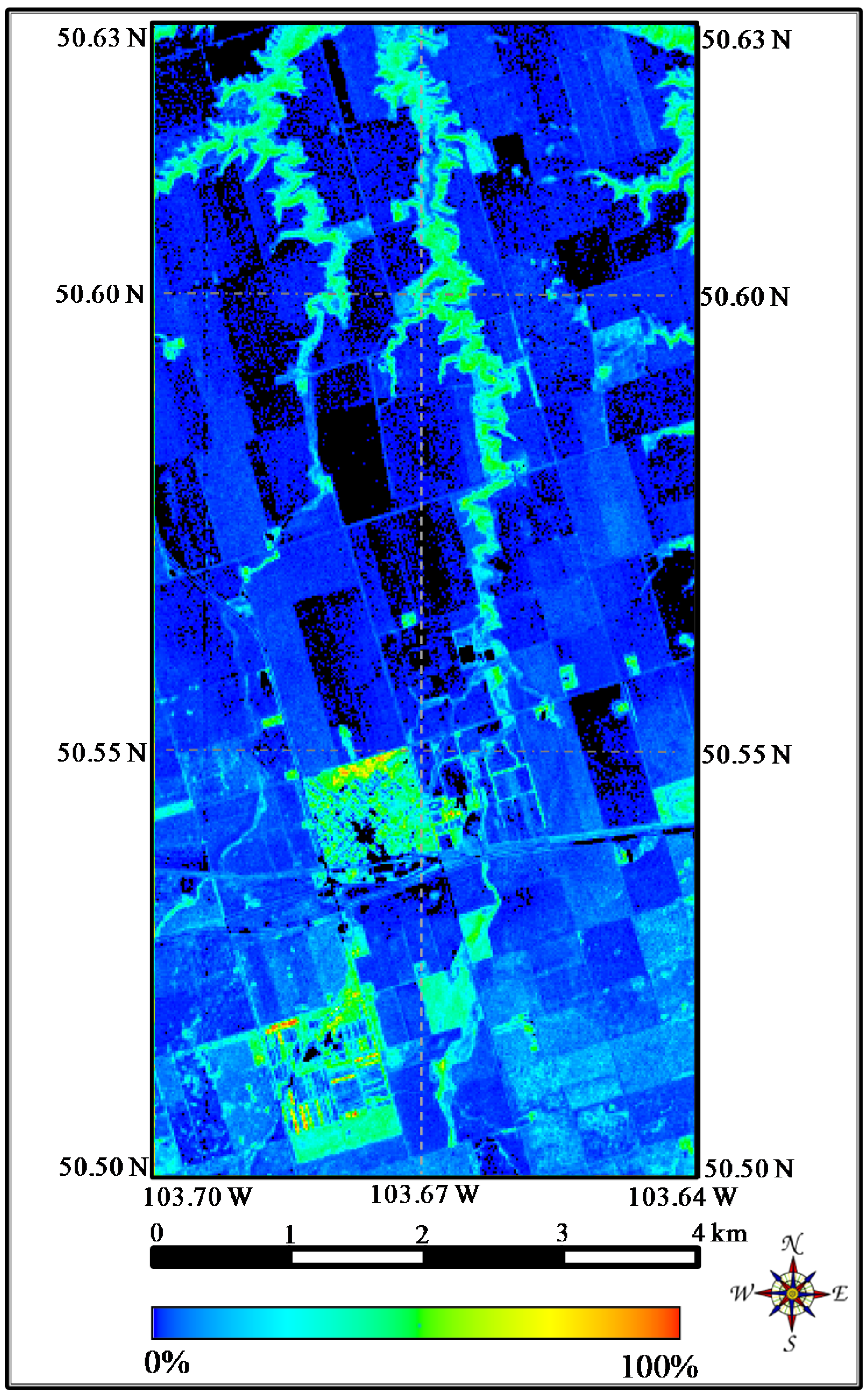
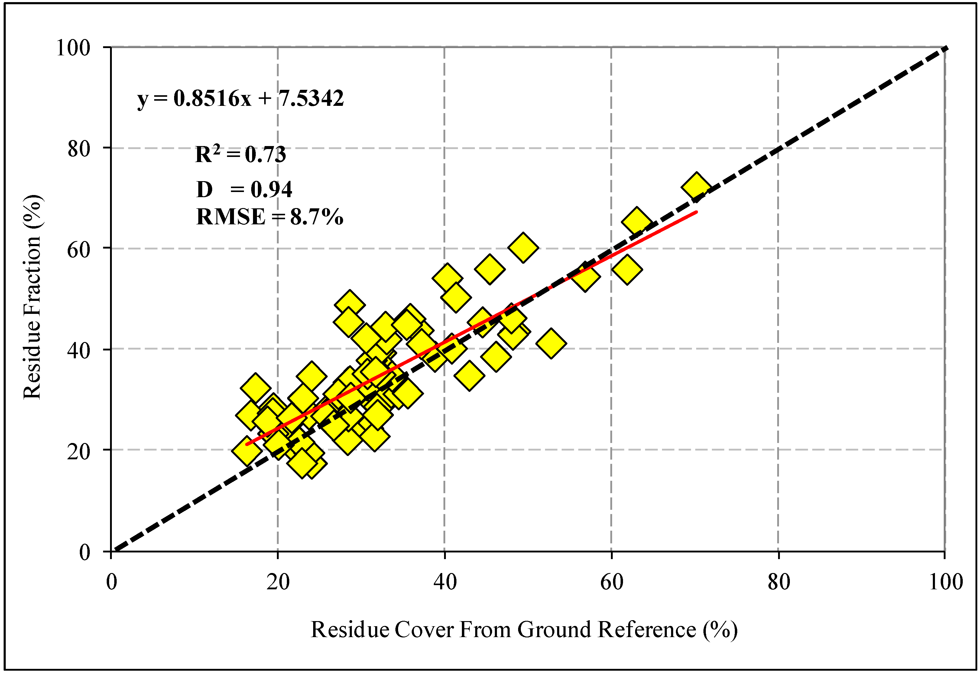
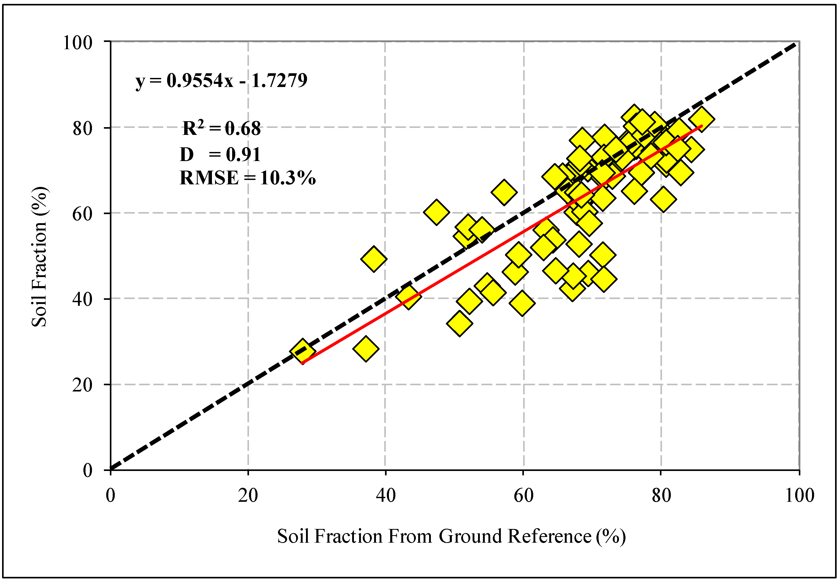
3. Results and Discussion

Figure 4 illustrates the endmember spectra used for the CLSMA: dry and slightly moist wheat residue, dry and slightly moist dark soils, and vegetation. The residue spectrum is similar to the soil spectra in the VNIR region of the electromagnetic spectrum and differs only in amplitude. However, in addition to the amplitude difference, the spectral shape is also considerably dissimilar in the SWIR region (1600 nm–2400 nm). The wetness reduced the amplitude of the spectral signature of the residue and soil across all wavelengths. The two considered spectra for soil show the same signature with a little difference in amplitude, likely due to differences in their color and moisture content. The dry and slightly moist residue spectrum shows the typical cellulose absorption features around 2100 nm, 2280 nm and 2340 nm, while the lignin absorption features are located around 1680 nm, 2270 nm, 2330 nm and 2380 nm. These absorption features are absent in the soil and vegetation spectra and offer the possibility to discriminate among residue, soil and green vegetation. Similar observations have also been made by Daughtry [69] and Bannari et al. [1,70]. Although only bare soil and crop residue were present, and there was no crop development in this period of the year, a green vegetation endmember was considered from our spectral library to deal with the coniferous trees in the scene (Figure 2d).
In order to extract the crop residue fractions, the image reflectance cube was unmixed considering the entire spectral range from 428 nm to 2355 nm. The PCRC derived from the CLSMA was validated against the percent cover estimated from ground vertical photographs (PCRCG). The relationship between the two variables was established and statistics were generated. Figure 5 and Figure 6 show the derived fraction maps for residue and vegetation from the Hyperion EO-1 data. Pixels with blue and red color represent the very low (0%) and very high (100%) percent crop residue and vegetation cover, respectively. Figure 5 presents a very good spatial distribution and variability of residue within the fields. Independent of the crop residue fraction and using ground reference measurements and GPS localization, the spatial variability of the ground-reference measurements was similar to the spatial variability found in the fractions derived from the hyperspectral data.
Figure 4. Endmember spectra convolved with the band centers of the Hyperion EO-1 sensor and used for Constrained Linear Spectral Mixture Analysis (CLMSA).
Remotesensing 07 08107 g004
Figure 5. Percent crop residue cover (PCRC) map derived from the Hyperion cube using CLMSA. The fraction map represents the dry and slightly moist residues.
Remotesensing 07 08107 g005
Figure 6. Vegetation cover fraction map derived from the Hyperion cube using CLMSA.
Remotesensing 07 08107 g006
The correlation between PCRC retrieved from the Hyperion data and PCRCG ground reference values calculated from ground vertical photographs shows a good index of agreement (D = 0.94) with a low RMSE (8.7%). The scatter plot, as presented in Figure 7, reveals a good linear relationship between the two variables (R2 of 0.73) and a good spatial variability (15%–75%). The PCRC between 18% and 45% was overestimated for the majority of the sampling points. This is probably due to the fact that only the endmember of wheat residue was considered, which is most abundant in the scene. In the study area, different crop residue types, such as canola, barley and corn, was found. However, they were distributed very sparsely and degraded, and, therefore, it was not possible to measure representative spectra for these residue classes in the field, as well this type of residue does not exist in our spectral libraries. The use of a specific endmember representing these crop residues type may relatively improve the results. The contribution of the shadow component was not significant or completely absent in this study. Therefore, it does not influence the results, because the image data were acquired early at the beginning of the agricultural season without any crop development. The localization of the ground sampling points in the Hyperion imagery and classifying the ground photos could be also a source of this small overestimation. On the other hand, according to the method described by Pacheco et al. [61], the endmember spectra were selected and extracted manually within the reflectance cube itself, representing the real image and field conditions. Unfortunately, the results did not improve because not all the selected wheat residue pixels were completely pure. Nevertheless, despite this small absolute difference (Figure 7), the relationship between the PCRC estimated from Hyperion data and PCRCG ground reference values is generally modeled satisfactorily.
Figure 7. Relationship between percent crop residue cover (PCRC) derived from Hyperion data and the ground-reference measurements (PCRCG). The black line represents the 1:1 line and the red one indicates the regression line.
Remotesensing 07 08107 g007
Figure 8 shows the relationship between the percent soil cover (PSC) derived from the Hyperion data and the ground-based photographs (PSCG). Compared to the ground-reference data, the model was overall a good predictor for soil percent cover with an index of agreement (D) of 0.91, a RMSE of 10.3% and a R2 of 0.68. The scatter plot, depicting the relationship between PSC and PSCG, clearly illustrates in general a good fit to the 1:1 line. However, the percent soil cover between 50% and 85% was underestimated, resulting in the data not fitting the 1:1 line very well. This is likely due to the fact that the selected soil endmember was probably not representative of all existing soils in the study area. The slope and the intercept corroborate these conclusions by expressing a little deviation from the 1:1 line. In addition, scaling issues between the endmembers collected in the field and the Hyperion image data being unmixed might play a role as discussed in [71]. Selecting and measuring other soil endmembers in the field with a different color and brightness would increase the fractions’ accuracy. The selection of endmembers, which truly represent the crop residue and soil conditions, is crucial for proper unmixing. In order to minimize errors in selecting endmembers, “pure” patches were considered for residue and soil before the data acquisition. However, these endmembers were probably not perfectly representative of the different soil types found in the experimental fields. In fact, small changes might occur within the test site, which could affect the spectral signature of soil. For example, changes in mineral composition, color, brightness, moisture, organic matter content and texture, etc. are factors, which influence the soil spectrum [72,73,74]. In addition, pre-processing of the Hyperion data is essential and will affect the integrity of the surface reflectance retrieval from the at-sensor radiance data cube. The sources of errors in the data pre-processing were reduced significantly by applying different techniques for the removal of sensor artifacts. However, it is probable that residual errors persist, causing a small difference between the measured endmembers in the field and their homologous position in the image.
Figure 8. Relationship between percent soil cover (PSC) derived from Hyperion data and the ground reference measurements (PSCG). The black line represents the 1:1 line and the red one indicates the regression line.
Remotesensing 07 08107 g008

4. Conclusions

The capability of the Hyperion EO-1 hyperspectral sensor was evaluated for estimating and mapping crop residue and soil fractions on agricultural land using CLSMA. The Hyperion data were corrected for the sensor spatial shift between the VNIR and SWIR detectors, image striping, dead pixels, and gain and offset errors, and reduced for noise in the imagery. The data were then atmospherically corrected and transformed to surface reflectance, while removing sensor smile at the same time. In a final preprocessing step, the data were post-processed to remove residual errors, and geometrically rectified as well. In order to extract the crop residue fraction, the image was unmixed considering the entire spectral range (427 nm–2355 nm) and the endmembers. These were simultaneously collected in the field with the Hyperion data from different targets using a GER-3700 spectroradiometer. The results showed that the acquired Hyperion data at the beginning of the agricultural season performed well. This good performance of Hyperion is due to the spectral band characteristics, especially the availability of contiguous narrow bands in the SWIR region, which is sensitive to the residue (lignin and cellulose absorption features) and soil. Correlation between ground-references measurements and extracted fractions from Hyperion data using CLSMA showed that overall the model was a good predictor for crop residue percent cover (D of 0.94, RMSE of 8.7%, and R2 of 0.73) and soil percent cover (D of 0.91, RMSE of 10.3% and R2 of 0.68). However, the endmember selection is a crucial step for proper unmixing. In order to minimize errors and to increase the estimation accuracy, endmembers must be selected carefully to represent different soil and residue types, which are available in the experimental fields. Indeed, changes in the soil mineral composition (color, brightness, moisture, organic matter content and texture, etc.) or in the residue conditions (type, degradation, density, etc.) influence the shape and amplitude of endmembers and, consequently, the extracted fractional cover.

Acknowledgments

The authors would like to thank the National Science and Engineering Research Council (NSERC) Canada and the Arabian Gulf University for their financial support. They acknowledge the support of the Canada Centre for Remote Sensing (CCRS), Natural Resources Canada, which provided the hyperspectral Hyperion data. Our gratitude to numerous people who were involved in this project and who provided their support and expertise: Lixin Sun (CCRS), Jean-Claude Deguise (CCRS, Robert Neville (CCRS), Rob Hitchcock (Department of National Defence) and all the field teams at Indian Head. Finally, we express gratitude to the anonymous reviewers for their constructive comments.

Author Contributions

A. Bannari performed the paper concept, field data acquisition, analysis and wrote the first draft of the paper. K. Staenz performed data analysis and provided feedback and contributions to the written paper. K. Champagne participated in the processing steeps and figures preparation. K. Shahid Khurshid participated in the field data acquisition and Hyperion data preprocessing.

Conflicts of Interest

The authors declare no conflict of interest.

References

  1. Bannari, A.; Haboudane, D.; Bonn, F. Intérêt du moyen infrarouge pour la cartographie des résidus de cultures. Can. J. Remote Sens. 2000, 26, 384–393. [Google Scholar] [CrossRef]
  2. Daughtry, C.S.T.; Hunt, E.R., Jr.; Doraiswamy, P.C.; McMurtrey, J.E. Remote sensing the spatial distribution of crop residues. Agron. J. 2005, 97, 864–871. [Google Scholar] [CrossRef]
  3. Daughtry, C.S.T.; Beeson, P.C.; Milak, S.; Akhmedov, B.; Sadeghi, A.M.; Hunt, E.R.; Tomer, M.D. Assessing the extent of conservation tillage in agricultural landscapes. Proc. SPIE 2012, 8531. [Google Scholar] [CrossRef]
  4. Zheng, B.; Campbell, J.B.; Serbin, G.; Galbraith, J.M. Remote sensing of crop residue and tillage practices: Present capabilities and future prospects. Soil Tillage Res. 2014, 138, 26–34. [Google Scholar] [CrossRef]
  5. Aase, J.K.; Tanaka, D.L. Reflectance from four wheat residues cover densities as influenced by three soil backgrounds. Agron. J. 1991, 83, 753–757. [Google Scholar] [CrossRef]
  6. Rice, C.W. Storing carbon in soil: Why and how? Geotimes 2002, 47, 1–5. [Google Scholar]
  7. Major, D.J.; Larney, F.L.; Lindwall, C.W. Spectral reflectance characteristics of wheat residues. In Proceedings of International Geoscience and Remote Sensing Symposium, Washington, DC, 20–24 May 1990; Volume 1, pp. 603–607.
  8. McNairn, H.; Protz, R. Mapping corn residues cover on agricultural fields in oxford county, ontario, using thematic mapper. Can. J. Remote Sens. 1993, 19, 152–159. [Google Scholar] [CrossRef]
  9. Biard, F.; Bannari, A.; Bonn, F. Soil Adjusted Corn Residues Index (SACRI): Un Indice Utilisant le Proche et le Moyen Infrarouge Pour la Détection de Résidus de Cultures de Maïs. In Proceedings of 17ème Symposium Canadien sur la Télédétection, Saskatoon, SK, Canada, 13–15 June 1995; pp. 413–419.
  10. Daughtry, C.S.T.; McMurtrey, J.E.; Chapelle, E.W.; Hunter, W.J.; Steiner, J.L. Measuring crop residues cover using remote sensing techniques. Theor. Appl. Climatol. 1996, 54, 17–26. [Google Scholar] [CrossRef]
  11. Biard, F.; Baret, F. Crop residues estimation using multiband reflectance. Remote Sens. Environ. 1997, 59, 530–536. [Google Scholar] [CrossRef]
  12. Bannari, A.; Haboudane, D.; McNairn, H.; Bonn, F. Modified soil adjusted crop residue index (msacri): A new index for mapping crop residue. In Proceedings of the IGARSS’2000, IEEE Geoscience and Remote Sensing Society, The Role of Remote Sensing in Managing the Global Environment, Honolulu, HI, USA, 24–28 July 2000; pp. 2936–2938.
  13. Ren, H.; Zhou, G. Estimating senesced biomass of desert steppe in Inner Mongolia using field spectrometric data. Agric. Forest Meteorol. 2012, 161, 66–71. [Google Scholar] [CrossRef]
  14. Bannari, A.; Chevrier, M.; Staenz, K.; McNairn, H. Potential of hyperspectal indices for estimating crop residue cover. Rev. Télédétect. 2008, 7, 447–463. [Google Scholar]
  15. Chevrier, M. Potentiel de la télédétection hyperspectrale pour la cartographie des résidus de cultures. Master’s Thesis, Geography Department, University of Ottawa, Ottawa, ON, Canada, 2002. [Google Scholar]
  16. Bannari, A.; Chevrier, M.; Deguise, J.-C.; McNairn, H.; Staenz, K. Senescent vegetation mapping using artificial neutral networks and hyperspectral remote sensing. In Proceedings of the International Geoscience and Remote Sensing Symposium (IGARSS), Toulouse, France, 21–25 July 2003; Volume 7, pp. 4292–4294.
  17. Daughtry, C.S.T.; Doraiswamy, P.C.; Hunt, E.R., Jr.; Stern, J.E.; McMurtrey, J.E.; Prueger, J.H. Remote sensing of crop residues cover and soil tillage intensity. Soil Tillage Res. 2006, 91, 101–108. [Google Scholar] [CrossRef]
  18. Bannari, A.; Pacheco, A.; Staenz, K.; McNairn, M.; Omari, K. Estimating and mapping crop residue cover in agricultural lands using hyperspectral and IKONOS images. Remote Sens. Environ. 2006, 104, 447–459. [Google Scholar] [CrossRef]
  19. Varshney, P.K.; Arora, M.K. (Eds.) Advanced Image Processing Techniques for Remotely Sensed Hyperspectral Data; Springer Verlag: Berlin/Heidelberg, Germany, 2004.
  20. Staenz, K. A decade of imaging spectrometry in Canada. Can. J. Remote Sens. 1992, 18, 187–197. [Google Scholar] [CrossRef]
  21. Thenkabail, P.S.; Gumma, M.K.; Teluguntla, P.; Irshad, A.; Mohammed, I.A. Hyperspectral remote sensing of vegetation and agricultural crops. Photogramm. Eng. Remote Sens. 2014, 80, 697–709. [Google Scholar]
  22. Curran, P.J. Imaging spectrometry. Prog. Phys. Geogr. 1994, 18, 247–266. [Google Scholar] [CrossRef]
  23. Staenz, K.; Mueller, A.; Uta Heiden, U. Overview of terrestrial imaging spectroscopy missions. In Proceedings of the International Geoscience and Remote Sensing Symposium (IGARSS’13), Melbourne, Australia, 21–26 July 2013; pp. 3502–3505.
  24. Adams, J.B.; Smith, M.O.; Gillepsie, A.R. Imaging spectroscopy: Interpretation based on spectral mixture analysis. In Remote Geochemical Analysis: Elemental and Mineralogical Composition; Pieters, C.M., Englert, P.A.J., Eds.; Cambridge University: Cambridge, UK, 1993; pp. 145–166. [Google Scholar]
  25. Thenkabail, P.S.; Lyon, J.G.; Huete, A. Hyperspectral Remote Sensing of Vegetation; CRC Press, Taylor and Francis Group: New York, USA, 2011. [Google Scholar]
  26. Goetz, A.F.H.; Vane, G.; Solomon, J.E.; Rock, B.N. Imaging spectrometry for earth remote sensing. Science 1985, 228, 1147–1153. [Google Scholar] [CrossRef] [PubMed]
  27. Staenz, K. Classification of a hyperspectral agriculture data set using band moments for reduction of the spectral dimensionality. Can. J. Remote Sens. 1996, 22, 248–257. [Google Scholar] [CrossRef]
  28. Staenz, K.; Szeredi, T.; Schwarz, J. ISDAS A system for processing and analyzing hyperspectral data. Can. J. Remote Sens. 1998, 42, 99–113. [Google Scholar] [CrossRef]
  29. Staenz, K.; Nadeau, C.; Secker, J.; Budkewitsch, P. Spectral unmixing applied to vegetated environments in the Canadian Arctic for mineral mapping. In Proceedings of the XIX ISPRS Congress, Amsterdam, The Netherlands, 16–23 July 2000.
  30. Adams, J.B.; Smith, M.O.; Johnson, P.E. Spectral mixture modeling: A new analysis of rock and soil types at Viking Lander. J. Geophys. Res. 1986, 91, 8113–8125. [Google Scholar] [CrossRef]
  31. Boardman, J.W. Analysis, understanding and visualization of hyperspectral data convex sets in N-Space. Proc. SPIE 1995, 2480, 14–20. [Google Scholar]
  32. Tompkins, S.; Mustard, J.F.; Pieters, C.M.; Forsyth, D.W. Optimization of endmembers for spectral mixture analysis. Remote Sens. Environ. 1997, 59, 472–489. [Google Scholar] [CrossRef]
  33. Neville, R.A.; Staenz, K.; Szeredi, T.; Lefebvre, J.; Hauff, P. Automatic endmember extraction from hyperspectral data for mineral exploration. In Proceedings of the Fourth International Airborne Remote Sensing Conference and Exhibition and the 21st Symposium on Remote Sensing, Ottawa, ON, Canada, 21–24 June 1999; Volume 2, pp. 891–897.
  34. García-Haro, F.J.; Gilabert, M.A.; Meliá, J. Extraction of endmembers from spectral mixtures. Remote Sens. Environ. 1999, 68, 237–253. [Google Scholar] [CrossRef]
  35. Feng, J.; Rivard, B.; Sánchez-Azofeifa, A. The topographic normalization of hyperspectral data: Implications for the selection of spectral end members and lithologic mapping. Remote Sens. Environ. 2003, 85, 221–231. [Google Scholar] [CrossRef]
  36. Beck, R. EO-1 User Guide, Version 2.3. Available online: http://eo1.usgs.gov and http://eo1.gsfc.nasa.gov; (accessed on 15 October 2015).
  37. NASA Sensors-Hyperion. Available online: http://eo1.usgs.gov/sensors/hyperion (accessed on 15 October 2015).
  38. Khurshid, K.S.; Staenz, K.; Sun, L.; Neville, R.; White, H.P.; Bannari, A.; Champagne, C.M.; Hitchcock, R. Preprocessing of EO-1 hyperion data. Can. J. Remote Sens. 2006, 32, 84–97. [Google Scholar] [CrossRef]
  39. Kruse, F.A.; Boardman, J.W.; Huntington, J.F. Comparison of airborne hyperspectral data and EO-1 hyperion for mineral mapping. IEEE Trans. Geosci. Remote Sens. 2003, 41, 1388–1400. [Google Scholar] [CrossRef]
  40. Sun, L.; Neville, R.A.; Staenz, K.; White, H.P. Automatic destriping of hyperion imagery based on spectral moment matching. Can. J. Remote Sens. 2008, 34, 68–81. [Google Scholar] [CrossRef]
  41. USGS, Earth Observing-1. Available online: http://eo1.usgs.gov/sensors/hyperioncoverage (accessed on 15 October 2015).
  42. Neville, R.A.; Sun, L.; Staenz, K. Spectral calibration of imaging spectrometers by atmospheric absorption feature matching. Can. J. Remote Sens. 2008, 34, 29–42. [Google Scholar] [CrossRef]
  43. Neville, R.A.; Sun, L.; Staenz, K. Detection of keystone in imaging spectrometer data. Proc. SPIE 2004, 5425. [Google Scholar] [CrossRef]
  44. Richter, N. Delineation of the Kam Kotia Mine Tailings Areas (Ontario, Canada) Using Hyperspectral TRWIS III Data. Master’s Thesis, Faculty of Mathematics and Natural Sciences, Institute for Geoecology, University of Potsdam, Potsdam, Germany, 2004. [Google Scholar]
  45. Berk, A.; Anderson, G.P.; Acharya, P.K.; Chetwynd, J.H.; Bernstein, L.S.; Shettle, E.P.; Matthew, M.W.; Adler-Golden, S.M. MODTRAN 4 User’s Manual; Air Force Research Laboratory: Hanscom AFB, MA, USA, 1999. [Google Scholar]
  46. Staenz, K.; Williams, D.J. Retrieval of Surface Reflectance from Hyperspectral Data Using a Look-Up Table Approach. Can. J. Remote Sens. 1997, 23, 354–368. [Google Scholar] [CrossRef]
  47. Green, R.O.; Conel, J.E.; Margolis, J.S.; Brugge, C.J.; Hoover, G.L. An inversion algorithm for the retrieval of atmospheric and leaf water absorption from AVIRIS radiance with compensation for atmospheric scattering. In Proceedings of the Third Annual Airborne Visible/Infrared Imaging Spectrometer (AVIRIS) Workshop, Pasadena, CA, USA, 20–21 May 1991; Volume 91, pp. 51–61.
  48. Gao, B.C.; Goetz, A.F.H. Column atmospheric water vapor and vegetation liquid water retrieval from Airborne Imaging Spectrometer data. J. Geophys. Res. 1990, 95, 3549–3564. [Google Scholar] [CrossRef]
  49. Staenz, K.; Neville, R.A.; Levesque, J.; Szeredi, T.; Singhroy, V.; Borstad, G.A.; Hauff, P. Evaluation of CASI and SFSI hyperspectral data for environmental and geological applications—Two case studies. Can. J. Remote Sens. 1999, 25, 311–322. [Google Scholar] [CrossRef]
  50. Champagne, C. Remote Sensing of Plant Water Content for Precision Agriculture: the Potential for Hyperspectral Modelling. Master’s Thesis, Geography Department, University of Ottawa, Ottawa, ON, Canada, 2002. [Google Scholar]
  51. PCI Geomatics. Tutorials; PCI Geomatics: Richmond Hill, ON, Canada, 2015; Available online: http://www.pcigeomatics.com/resources-support/geomatica/tutorials.pdf (accessed on 15 February 2015).
  52. Geophysical and Environmental Research Corporation. GER 3700 Spectroradiometer User’s Manual Version 2.1; Millbrook: New York, USA, 1990. [Google Scholar]
  53. Wang, L.; He, D.C.; Baulu, T. Unsupervised classification of remotely sensed multispectral image data. Can. J. Remote Sens. 1992, 8, 174–178. [Google Scholar] [CrossRef]
  54. Labsphere, A. Guide to Reflectance Coatings and Materials, North Sutton, New Hampshire. Available online: http://www.labsphere.com/tech_info/docs/Coating_&_Material_Guide.pdf (accessed on 15 October 2014).
  55. Jackson, R.D.; Pinter, P.J.; Paul, J.; Reginato, R.J.; Robert, J.; Idso, S.B. Hand-Held Radiometry—A Set of Notes Developed for Use at the Workshop on Hand-Held Radiometry Phoenix, Ariz., February 25-26, 1980; Agricultural Reviews and Manuals; ARM-W-19; U.S. Department of Agriculture Science and Education Administration: Phoenix, AZ, USA, 1980. [Google Scholar]
  56. Cyr, L.; Bonn, F.; Pesant, A. Vegetation indices derived from remote sensing for estimation of soil protection against water erosion. Ecol. Model. 1995, 79, 277–285. [Google Scholar] [CrossRef]
  57. Arsenault, É.; Bonn, F. Evaluation of soil erosion protective cover by crop residues using vegetation indices and spectral mixture analysis of multispectral and hyperspectral data. In Proceedings of the 23rd Canadian Symposium on Remote Sensing, Canadian Remote Sensing Society, Ottawa, ON, Canada, 21–24 August 2001; pp. 299–308.
  58. Zhang, L.; Li, D.; Tong, Q.; Zheng, L. Study of the spectral mixture model of soil and vegetation in PoYang Lake area, China. Int. J. Remote Sens. 1998, 19, 2077–2084. [Google Scholar] [CrossRef]
  59. Peddle, D.R.; Hall, F.G.; LeDrew, E.F. Spectral mixture analysis and geometric-optical reflectance modeling of boreal forest biophysical structure. Remote Sens. Environ. 1999, 67, 288–297. [Google Scholar] [CrossRef]
  60. Lévesque, J.; King, D.J. Spatial analysis of radiometric fractions from high-resolution multispectral imagery for modelling individual tree crown and forest canopy structure and health. Remote Sens. Environ. 2003, 84, 586–602. [Google Scholar] [CrossRef]
  61. Pacheco, A.; Bannari, A.; Staenz, K.; McNairn, H. Deriving percent crop cover over agriculture canopies using hyperspectral remote sensing. Can. J. Remote Sens. 2008, 34, 110–123. [Google Scholar] [CrossRef]
  62. Schwarz, J. Classification of Hyperspectral Data. Master’s Thesis, School of Computer Science, Carleton University, Ottawa, ON, Canada, 1998. [Google Scholar]
  63. Myneni, R.B.; Maggion, S.; Jaquinta, J.; Privette, J.L.; Gordon, N.; Pinty, B.; Kimes, D.S.; Verstraete, M.M.; Williams, D.L. Optical remote sensing of vegetation: modeling, caveats, and algorithms. Remote Sens. Environ. 1995, 51, 169–188. [Google Scholar] [CrossRef]
  64. Kerdiles, H.; Grondona, M.O. NOAA-AVHRR NDVI decomposition and subpixel classification using linear mixing in the Argentinean Pampa. Int. J. Remote Sens. 1995, 16, 1303–1325. [Google Scholar] [CrossRef]
  65. Boardman, J.W. Automating spectral unmixing of AVIRIS data using convex geometry. In Summaries of the 4th Airborne Geoscience Conference; Green, R.O., Ed.; JPL Jet Propulsion Laboratory: Pasadena, CA, USA, 1992; Volume 1, pp. 11–14. [Google Scholar]
  66. Endsley, H.H. Spectral unmixing algorithms based on statistical models. Proc. SPIE 1995, 2480, 14–22. [Google Scholar]
  67. Statistica Software. Available online: http://statistica.software.informer.com/10.0/ (accessed on 15 October 2014).
  68. Willmott, C.J. Some comments on the evaluation of model performance. Bull. Am. Meteorol. Soc. 1982, 63, 1309–1313. [Google Scholar] [CrossRef]
  69. Daughtry, C.S.T. Discriminating crop residues from soil by shortwave infrared reflectance. Agron. J. 2001, 93, 125–131. [Google Scholar] [CrossRef]
  70. Bannari, A.; Haboudane, D.; Bonn, F. Potentiel des mesures multispectrales pour la distinction entre les résidus de cultures et les sols nus sous-jacents. In Proceedings of Forth International Airborne Remote Sensing Conference and Exhibition/21st Canadian Symposium on Remote Sensing, Ottawa, ON, Canada, 21–24 June 1999; Volume 2, pp. 359–366.
  71. Shang, J.; Neville, R.A.; Staenz, K.; Sun, L.; Morris, B.; Howarth, P. Comparison of fully constrained and weakly constrained unmixing through mine-tailings composition mapping. Can. J. Remote Sens. 2008, 34, 92–109. [Google Scholar] [CrossRef]
  72. Irons, J.R.; Weismiller, R.A.; Petersen, G.W. Soil reflectance. In Theory and Applications of Optical Remote Sensing; Asrar, G., Ed.; Wiley-Interscience: New York, NY, USA, 1989; pp. 66–106. [Google Scholar]
  73. Bannari, A.; Huete, A.R.; Morin, D.; Zagolski, F. Effets de la couleur et de la brillance du sol sur les indices de végétation. Int. J. Remote Sens. 1996, 17, 1885–1906. [Google Scholar] [CrossRef]
  74. Huete, A.R. Soil influences in remotely sensed vegetation-canopy spectra. In Theory and Applications of Optical Remote Sensing; Asrar, G., Ed.; John Wiley & Sons, Inc.: New York, NY, USA, 1989; pp. 107–141. [Google Scholar]

