1. Introduction
Photographs have been widely used as documentary evidences in numerous fields of science since the invention of photography. In the case of Earth Sciences, photographs have been used to describe, analyze and quantify processes. Capturing photographs outdoor usually represents a challenge because light conditions cannot be controlled or programmed as in a laboratory experiment [
1]. The capture of images with high differences in the illumination of the brightest and the darkest parts of the scene (
i.e., scenes with High Dynamic Ranges or HDR) is not possible with conventional digital cameras available today. The dynamic range of an image can be defined as the ratio between areas with the highest and the lowest light intensity in the scene. In natural environments this figure can reach values around 500,000:1 [
2]. The amount of light received by the sensor inside a digital camera is controlled by the exposure time, which is the time that the shutter of the camera is opened. High exposure times usually result in photographs with details and textures in areas with low illumination while high illuminated areas are usually shown in a uniform white colour without details. On the other hand, low exposure times result in photographs with details and textures in zones highly illuminated while areas with low illumination are shown like uniform black colored parts. Therefore, it is not always possible to capture photographs in natural environments without losing details and texture in bright and dark areas due to overexposure (long exposure times) and underexposure (short exposure times), respectively.
Since the 90s, HDR procedures have been developed and applied successfully to overcome this limitation. HDR techniques are based in the use of multiple images of the same scene that have been captured from the same location but with different exposure times known as Low Dynamic Range images (LDR). Then, LDR images are combined in a unique scene selecting the most appropriate illumination for each pixel in the set of LDR images. The result is a HDR composition showing details in high and low illuminated features in the scene. This result can be exported as a radiance or a tone map to be used as a conventional picture within any software.
In the past five years, automatic photogrammetric procedures based on Structure from Motion and Multi-View Stereo techniques (SfM-MVS) have been widely explored and applied in the field of Earth Sciences, particularly in Geomorphology [
1,
3,
4,
5,
6,
7,
8,
9,
10]. The SfM [
11] technique solves the camera parameters and orientations and produces a sparse 3D point cloud of the scene. These clouds are commonly insufficiently detailed and noisy [
12] to be applied for geomorphological purposes. The MVS [
13] approach reduces the noise in the scene and densify the point cloud getting the number of points in the cloud to increase by two or three orders of magnitude [
3]. The advantages of SfM-MVS against other methods that offer similar accuracies have been highlighted by several researchers: accuracy, low cost and little expertise required as compared with more traditional techniques, [
1,
3,
14]. The accuracy of SfM-MVS approaches depends on several factors: average distance from the camera to the target, camera network geometry and characteristics, quality and distribution of the ground control points, software and illumination conditions. The SfM-MVS approaches are currently implemented in a wide variety of software packages and web services (e.g., Agisoft Photoscan [
15], Arc 3D [
16], Bundler and PMVS2 [
17], CMP SfM [
18], Micmac [
19], Photomodeler [
20], Visual SfM [
21], 123D Catch [
22],
etc.). Among these software packages Agisoft Photoscan (≈400 €) and 123D Catch (free available) are two interesting options. The 123D Catch software has been previously applied to estimate gully headcut erosion [
1], to reconstruct riverbank topography [
23], to generate Digital Elevation Models of a rock glacier [
10] and to measure coastal changes [
24]. Regarding Agisoft Photoscan, it has been previously used to estimate the mass balance of a small glacier [
25] or to carry out a multi-temporal analysis of landslide dynamics [
26]. Several works have tried to understand the relationship between the accuracy of SfM-MVS approaches and the different scales of work (plot, geomorphological feature, sub-basin, basin and landscape scale) [
3,
27]. Works analyzing the accuracy of a specific software are common, however researches comparing the performance of two or several packages, algorithms, workflows or pipelines applied to the same study area are scarce in the literature. [
8] is a recent exception where Visual SfM [
21] and Micmac [
19] are compared and used to monitor the displacement of a slow-moving slope movement. A general opinion among the scientific community is that the validation of SfM-MVS techniques, approaches and pipelines is just beginning and more examples are required to understand the frontiers and limitations of these methods.
Some SfM-MVS approaches have been validated robustly in recent works [
3,
27], however most of the validations are carried out with gridded data, a result of processing the point clouds (which are the primary result of the SfM-MVS methods) and using conventional statistics as the Root Mean Square Error (RMSE) calculated using a few points in the cloud-model. The use of rasterized surfaces is justified because most of the final derived or secondary products obtained from SfM-MVS raw data are Digital Elevation Models (DEMs) and derived attributes as gridded surfaces. However, these surfaces bind together errors of the SfM-MVS and the rasterization procedures and make it difficult to isolate the magnitude of each factor. The use of DEMs (or gridded surfaces) is related with the traditional work of geomorphologists with Geographical Information Systems (GIS) in a not real 3D environment. SfM-MVS primary data are 3D point clouds and an algorithm performing a test of the quality of point clouds in 3D is necessary [
14].
As stated before, in natural environments, shadows and materials with different illuminations are common and they cause errors or blind areas in the resulting photo-reconstructed 3D models. SfM-MVS software packages demand images with rich textures and poor textured scenes may produce outliers or large areas without data. The performance of SfM-MVS is based on identifying matching features in different images commonly using the Scale Invariant Feature Transform algorithm (SIFT) [
28]. Then, the matching features are used to iteratively solve the camera model parameters. Therefore, the final quality of the 3D model depends, among other factors, on the image texture of the surfaces in the scene [
29] because the matching algorithm works with image textures. Concurrently, image texture will depend on the complexity of the features, the lighting and the materials of every scene [
5]. In the field of geomorphological research, this problem has been documented. For example, some recent works [
1,
5,
30] showed problems in areas with dense and homogeneous vegetation cover and others [
31] talked about surfaces with bare sand, snow or other highly flat surfaces as candidates for poor results using SfM-MVS. The relationship between the quality of a DEM obtained by means of photo-reconstruction methods and the amount of shadowed-lighted areas in the photographs used as input in the photo-reconstruction procedure has been recently showed by [
10]. Additionally, the surficial cover of different geomorphological features can be highly variable in time. For instance, a riverbank can be bare, vegetated or covered by water in different times along the hydrological year. This variability results in quite different textures in the photographs and should be taken into account when estimating thresholds to quantify geomorphic changes. In the case of rock glaciers, strong changes in the light conditions and the materials covering the ice are experienced along the year. In this kind of geomorphological feature, debris or rocks cover the ice forming the glacier permanently. At the same time, this layer of rocks may be partially or totally covered by snow during a part of the year. Although the use of HDR techniques seems to be appropriate to improve the performance of SfM-MVS approaches, this hypothesis has not been tested yet [
32]. Point clouds obtained with HDR and LDR images were compared [
33] but authors did not use any benchmark model to estimate the degree of improvement, if any. They concluded that, geometrically, both point clouds were similar, although a visual qualitative enhancement of the contrast in the colour of the point cloud was observed. Other recent work tested whether the pre-processing of digital images with HDR techniques may improve 3D models of cultural heritage objects obtained by means of SfM-MVS techniques [
32]. Authors showed that point clouds generated using HDR compositions yielded 5% more points matched than point clouds obtained using LDR images for a ceramic object [
32]. In the case of a metallic object, the increase in the number of points matched was higher with 63% more than the point clouds generated using LDR images as input. In this work, authors did not test the geometrical accuracy of the point clouds generated using HDR compositions [
32]. Also recently, classical digital photogrammetry was fed with HDR images [
34] and later applied to measure geometry and light simultaneously in roadways [
35]. The results proved the usefulness of HDR approaches within the classical digital photogrammetry pipeline.
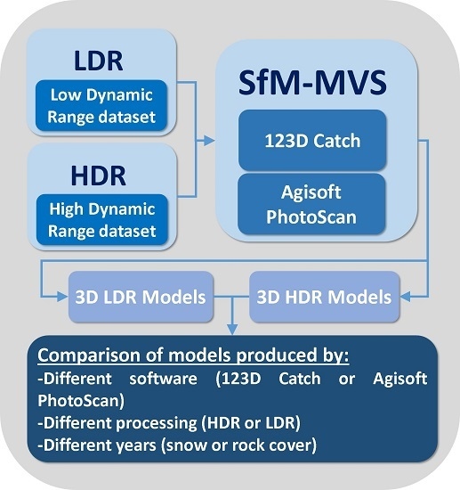
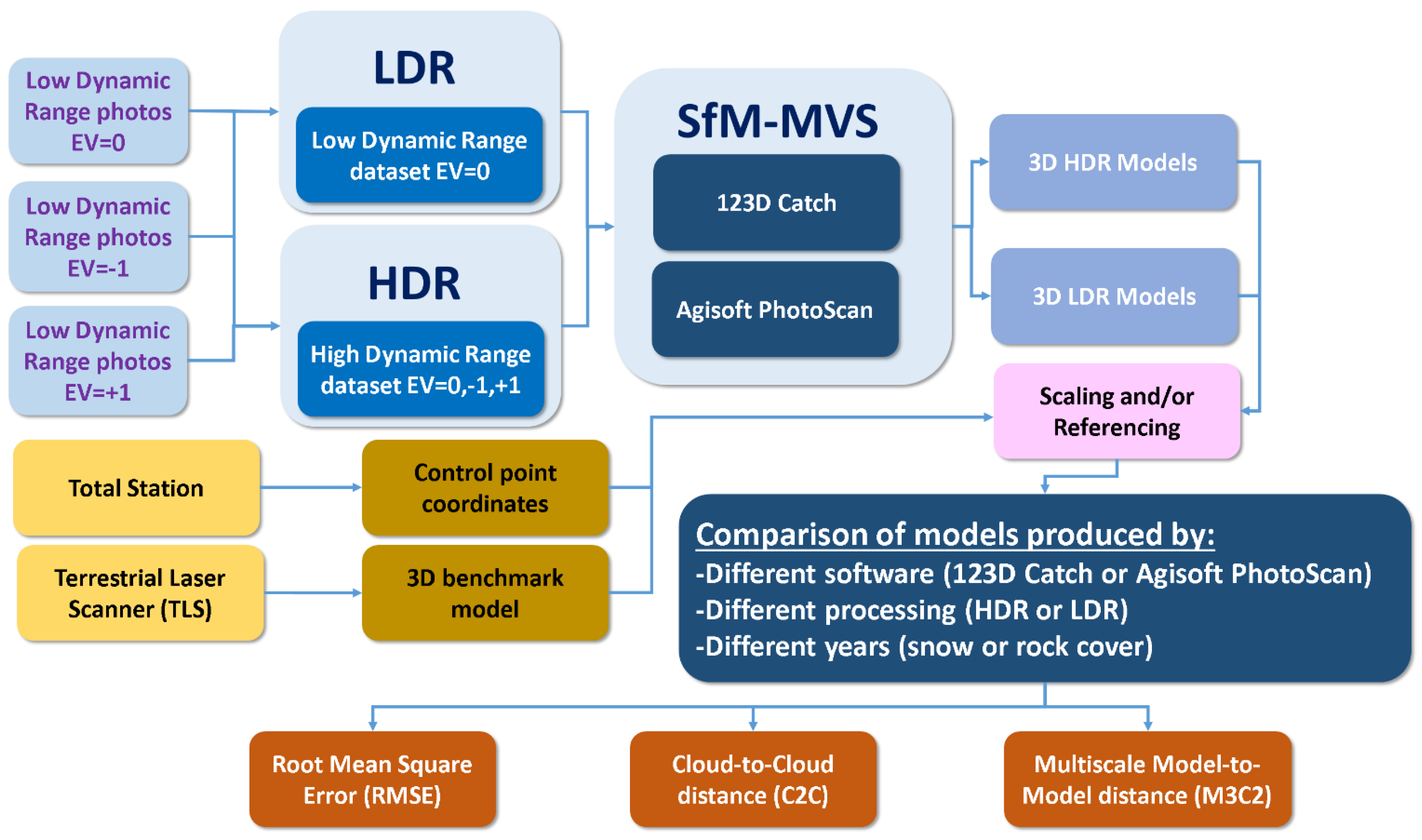
Therefore, the main objective of this work is to investigate the accuracy that can be obtained from different workflows for the 3D photo-reconstruction of the Corral del Veleta rock Glacier in Spain in three different years: 2011, 2012 and 2014. Specifically, the following issues were analyzed:
- -
The possibility of improving SfM-MVS techniques with the use of HDR tone mapped images.
- -
The accuracy of two different software packages commonly used to get 3D models of geomorphological features: 123D Catch [
22] and Agisoft Photoscan [
15].
- -
The influence of snow or debris cover in the accuracy of the resulting photo-reconstructions for the Corral del Veleta rock glacier.
The estimation of the accuracy of the point clouds will be carried out using traditional parameters, such as the RMSE, but also more specific and recently proposed 3D distance tests.
3. Results and Discussion
A total of 12 point clouds were produced by the SfM-MVS approaches, four each year of the study (2011, 2012 and 2014). Additionally, one point cloud was acquired by means of the TLS every year.
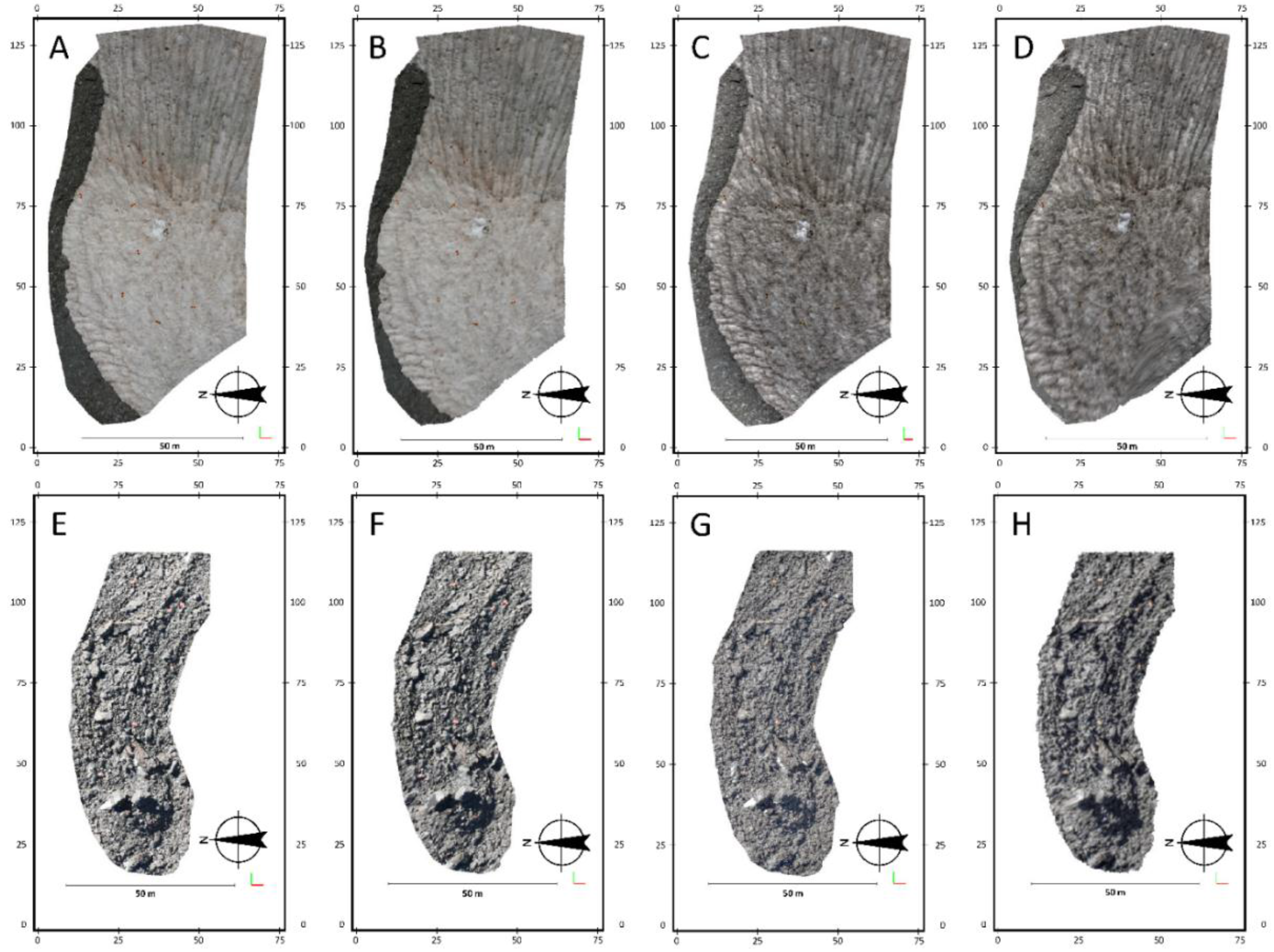
Figure 4 presents the photo-reconstructions of the glacier obtained with different pipelines for the years 2011 and 2014. Visually, important differences were observed between the point clouds generated with HDR and LDR images for the year 2011 (
Figure 4A–D), under snow cover conditions. In 2014, the resulting point clouds did not present important differences from a visual viewpoint (
Figure 4E–H) showing the debris cover of the glacier. Volumetric point densities for point clouds obtained by means of 123D Catch software were in the range of 1–100 points·m
−3 while clouds elaborated with Agisoft Photoscan median point densities varied from 1500 to 2000 points·m
−3.
Figure 4.
Resulting point clouds obtained with (A) Low Dynamic Range (LDR) images in Agisoft Photoscan for the year 2011, (B) LDR images in 123D Catch for the year 2011, (C) High Dynamic Range (HDR) images in Agisoft Photoscan for the year 2011, (D) HDR images in 123D Catch for the year 2011, (E) LDR images in Agisoft Photoscan for the year 2014, (F) LDR images in 123D Catch for the year 2014, (G) HDR images in Agisoft Photoscan for the year 2014 and (H) HDR images in 123D Catch for the year 2014.
Table 1 presents the camera calibration parameters and their adjusted values for the models produced by Agisoft Photoscan as 123D Catch software does not generate this information. Agisoft Photoscan produces a figure with the spatial distribution of image residuals, however, you can only get this information if the scaling and georeferencing of the model has been carried out within the software. In order to keep a methodological consistency to compare Agisoft Photoscan and 123D Catch the scaling and georeferencing was carried out using CloudCompare software.
Table 1.
Camera calibration parameters with their initial and adjusted values, where fx and fy are horizontal and vertical focal length (in pixels) respectively, cx and cy are the x and y coordinates of the principal point and k1, k2 and k3 are the radial distortion coefficients. The Skew and tangential distortion coefficients (p1 and p2) were set to 0 in the initial and the adjusted calibration model. Pixel size of 0.008 mm, focal length of 100 mm and the size of the picture (4386 × 2920 pixels) were constant values for all the surveys. Note that these parameters are only estimated for the point clouds obtained by means of Agisoft Photoscan (123D Catch does not produce this information) and the spatial distribution of image residuals report, which is typically produced by this software, is not available since the scaling and referencing was carried out using CloudCompare software.
| | LDR | | HDR |
|---|
| Initial | Adjust | Residual | | Initial | Adjust | Residual |
|---|
| 2011 | fx | 12161.8 | 12053.9 | 107.9 | | 12161.8 | 11996.2 | 165.6 |
| fy | 12161.8 | 12053.9 | 107.9 | | 12161.8 | 11996.2 | 165.6 |
| cx | 2184.00 | 2176.66 | 7.34 | | 2193.00 | 2144.20 | 48.80 |
| cy | 1456.00 | 1382.06 | 73.94 | | 1460.00 | 1451.36 | 8.64 |
| k1 | 0.0000 | −0.1802 | 0.1802 | | 0.0000 | −0.1783 | 0.1783 |
| k2 | 0.0000 | 1.0894 | −1.0894 | | 0.0000 | 0.7387 | −0.7387 |
| k3 | 0.0000 | −2.8829 | 2.8829 | | 0.0000 | −2.3432 | 2.3432 |
| 2012 | fx | 12161.8 | 12065.5 | 96.3 | | 12161.8 | 12069.7 | 92.1 |
| fy | 12161.8 | 12065.5 | 96.3 | | 12161.8 | 12069.7 | 92.1 |
| cx | 2184.00 | 2195.18 | −11.18 | | 2193.00 | 2204.01 | −11.01 |
| cy | 1456.00 | 1380.71 | 75.29 | | 1460.00 | 1388.51 | 71.49 |
| k1 | 0.0000 | −0.1498 | 0.1498 | | 0.0000 | −0.1545 | 0.1545 |
| k2 | 0.0000 | −0.1001 | 0.1001 | | 0.0000 | 0.2562 | −0.2562 |
| k3 | 0.0000 | 14.5264 | −14.5264 | | 0.0000 | −0.1545 | 0.1545 |
| 2014 | fx | 12161.8 | 12022.5 | 139.3 | | 12161.8 | 12030.5 | 131.3 |
| fy | 12161.8 | 12022.5 | 139.3 | | 12161.8 | 12030.5 | 131.3 |
| cx | 2184.00 | 2170.67 | 13.33 | | 2193.00 | 2175.77 | 17.23 |
| cy | 1456.00 | 1426.23 | 29.77 | | 1460.00 | 1433.24 | 26.76 |
| k1 | 0.0000 | −0.1548 | 0.1548 | | 0.0000 | −0.1472 | 0.1472 |
| k2 | 0.0000 | 0.3270 | −0.3270 | | 0.0000 | 0.0599 | −0.0599 |
| k3 | 0.0000 | 8.1385 | −8.1385 | | 0.0000 | 10.5228 | −10.5228 |
3.1. Global Structural Accuracy of the Point Clouds
The sources of error, and therefore inaccuracies, of the workflows presented in this work are mainly related to the following factors: the distance from the camera to the target [
3], the geometry of the capture [
25], the quality of the control points [
25] and the modelling procedure that is influenced by cover type and illumination conditions [
10,
29]. The distance from the camera to the target and the geometry of the capture are, in this case, imposed by the steep relief and will be discussed later using the survey range or the relative precision ratio figures. An assessment of the sources of error is discussed in the following sections where the values of the RMSE, C2C and M3C2 are presented. The consistency in the use of instruments, techniques and methods allows the analysis of the effect of the HDR pre-processing, the use of different software and the influence of different cover types.
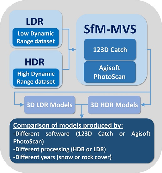
The quality of the control points (
Figure 2C) is mainly controlled by their spatial distribution and the characteristics of the instruments used for their measurement.
Figure 1B and
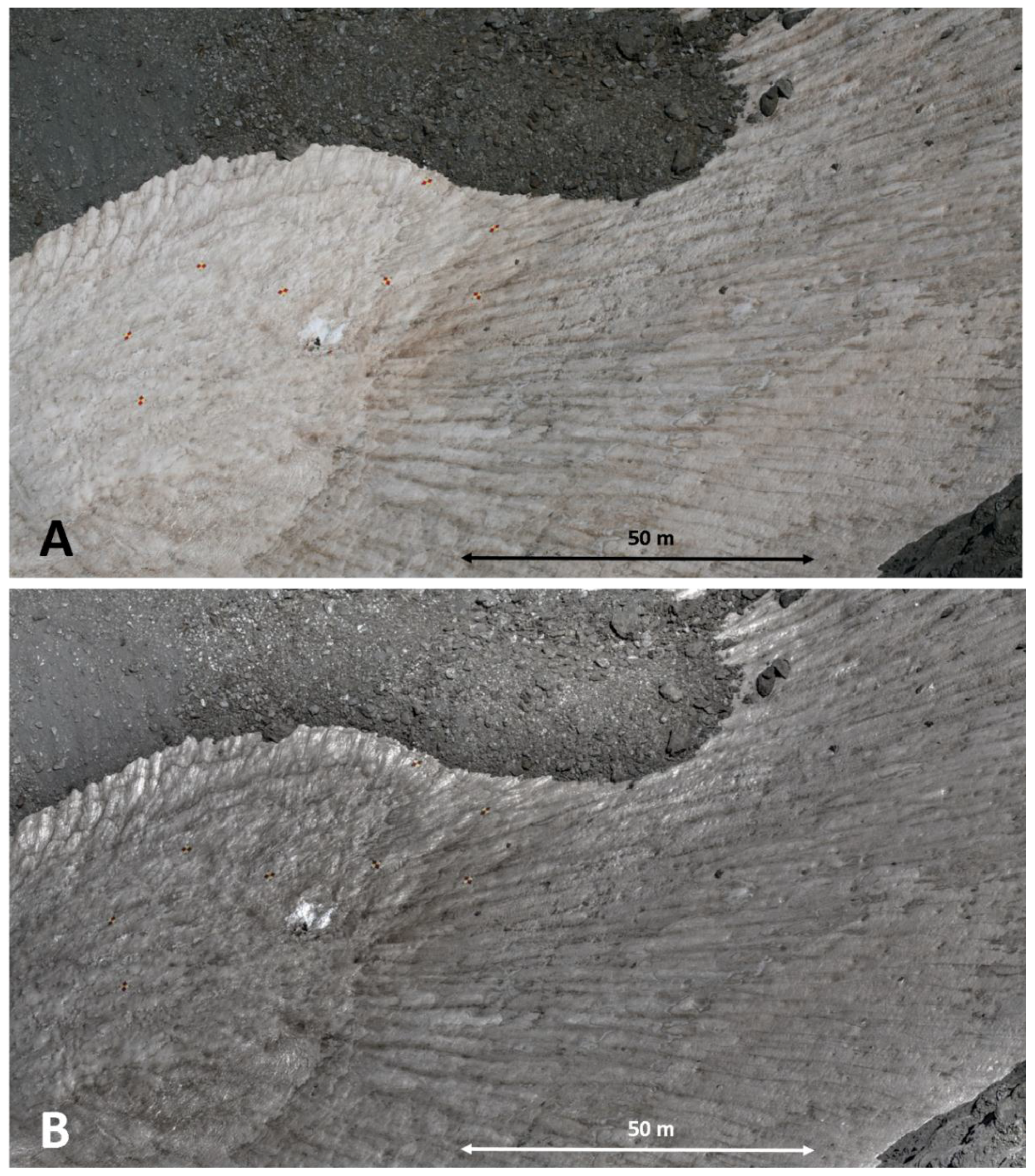
Figure 5A show the spatial distribution of the 10 control points over the glacier covering the front, the sites and the head. The measurement of their coordinates was carried out with a laser total station that ensures an accuracy <0.5 cm in every single point.
Figure 5.
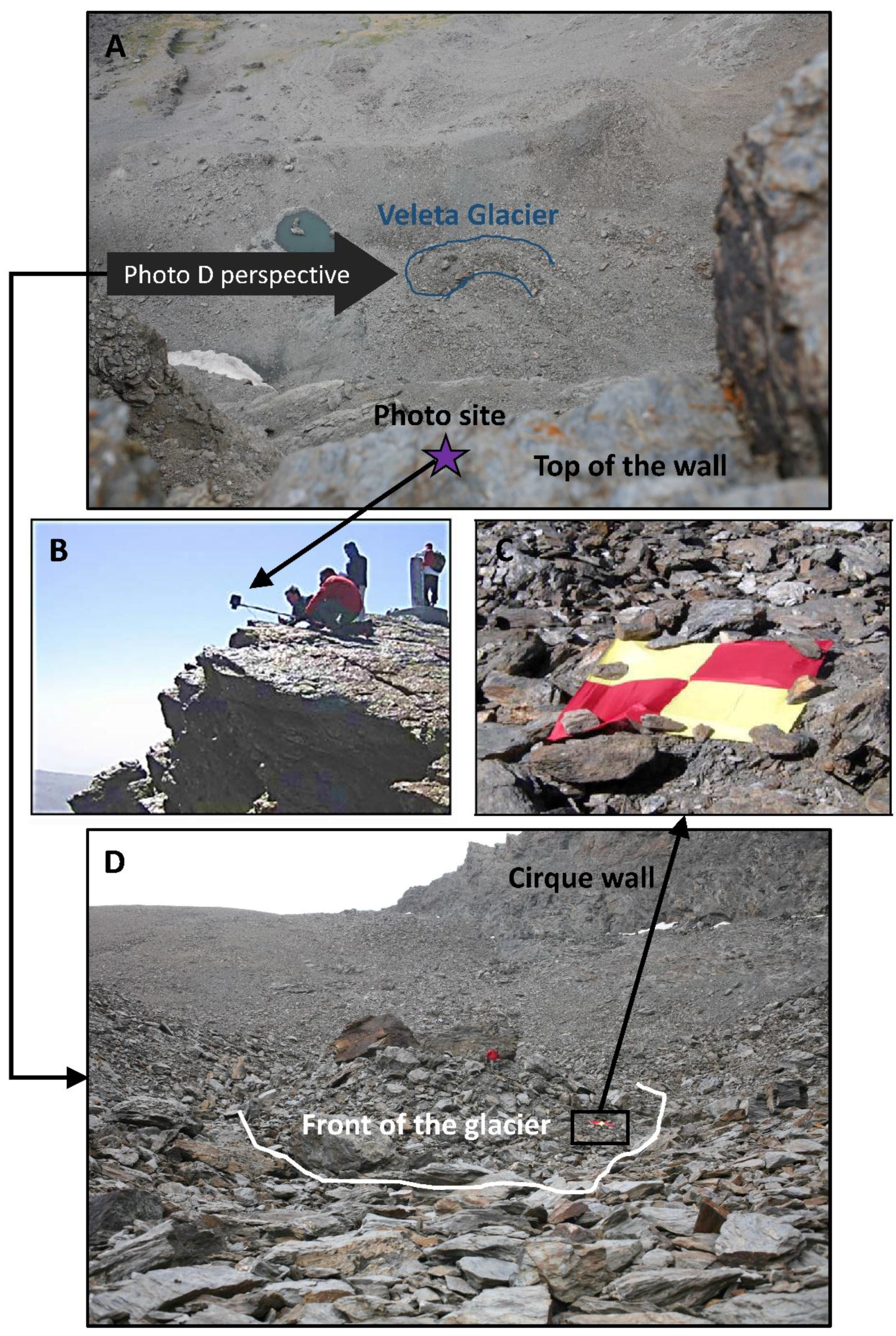
(A) Oblique Low Dynamic Range conventional image (LDR) and (B) oblique High Dynamic Range composition (HDR, i.e., elaborated with three conventional photographs acquired with Exposition Values of −1.00, 0.00 and +1.00) of the Corral del Veleta rock glacier in 2011. Control points can be observed in red and yellow color for both images. Note that these photographs are not orthorectified and referenced so only an approximate reference distance is shown in the figure.
Figure 5.
(A) Oblique Low Dynamic Range conventional image (LDR) and (B) oblique High Dynamic Range composition (HDR, i.e., elaborated with three conventional photographs acquired with Exposition Values of −1.00, 0.00 and +1.00) of the Corral del Veleta rock glacier in 2011. Control points can be observed in red and yellow color for both images. Note that these photographs are not orthorectified and referenced so only an approximate reference distance is shown in the figure.
Scaling and referencing errors quantified by the RMSE reflect how the resulting models fit to the relative coordinate system established by the control points and measured by means of the total station,
i.e., they are indicators of the global geometrical quality of the 3D model. If the control points present a good spatial distribution over the study area, the RMSE shows the global structural quality of the 3D model produced by the photo-reconstruction and can be an indicator of the presence of non-linear deformations. The RMSEs presented in
Table 2 show that the best performance was always produced by Agisoft Photoscan and in two out of three cases using as input conventional LDR images (acquired with EV = 0.00). On the other hand, the worst performance was produced by 123D Catch software using as input HDR compositions. The RMSEs for the different workflows ranged from 0.036 m (Agisoft Photoscan software with LDR images in 2011) to 2.469 m (123D Catch software with HDR images in 2012).
The average RMSEs for the years 2014 and 2012, were lower and slightly lower (respectively) as compared to the average RMSE for the year 2011 (
Table 2), when almost all the study area was covered by snow (
Figure 4). The residuals of the camera calibration parameters presented in
Table 1 also support this fact, however no statistical significant relationship was observed between the RMSE and the residuals of the different camera calibration parameters. Although the HDR pre-processing resulted in images with richer textures and a clear visual improvement of the features shown in the scene for the year 2011 (
Figure 5), no significant improvement was found out in the RMSE using this approach. This qualitative visual improvement has been observed by [
32,
33].
Table 2.
Root Mean Square Errors (RMSEs; in meters) obtained during the scaling and referencing of each point cloud.
Table 2.
Root Mean Square Errors (RMSEs; in meters) obtained during the scaling and referencing of each point cloud.
| | Software | 2011 | 2012 | 2014 | Average |
|---|
| Low Dynamic Range (LDR conventional) images | 123D Catch | 1.128 | 0.461 | 0.791 | 1.027 |
| Agisoft Photoscan | 0.036 | 0.341 | 0.261 | 0.213 |
| High Dynamic Range (HDR) images | 123D Catch | 2.374 | 2.469 | 1.067 | 1.978 |
| Agisoft Photoscan | 0.067 | 0.307 | 0.391 | 0.242 |
| Average | | 0.902 | 0.894 | 0.628 | |
The figures presented in
Table 2 result in an average ratio between RMSE and survey range of 1:370. In [
27], a brief summary of previous works that have estimated this parameter resulted in a median ratio between RMSE and survey range of 1:639. A previous work in the Corral del Veleta rock glacier [
10] presented values ranging from 1:1,071 to 1,429 but these values were calculated using the average C2C distance to the benchmark TLS model instead of using the RMSE and different pipelines. The dataset of RMSEs presented in
Table 2 add knowledge to the needed systematic validation of SfM-MVS in a wide variety of environments demanded by the scientific community [
27]. Although, it should be noted that the accuracies presented here could be improved because in this case the geometry of the pose is highly limited to a few locations in the top of the Corral del Veleta wall and the important differences in the survey range from 1:370 to the average figure of 1:639 for geomorphological features defined by [
27] can be attributed to this weak geometry of the camera locations. According to this figures, the weak imposed geometry of the capture would be reducing in a half the expected accuracy of the models in the case of the Veleta rock glacier. For sure, other factors are influencing the difference in the average survey range for geomorphological features presented in [
27] and the one estimated here, but it is hypothesized that an important increase in the accuracy of the models would be get with a convergent geometry of the pose. Camera network geometry has been recently supported as the main factor determining the quality of 3D models of a rock glacier by means of SfM-MVS techniques [
25]. [
10] validated two SfM-MVS approaches (a self-implemented algorithm and 123D Catch software) for the Corral del Veleta rock glacier finding out that only changes at sub-meter scale could be identified in a multi-temporal study according to the obtained differences with a TLS point cloud. The values of the RMSEs estimated here and presented in
Table 2 suggest that only relatively large changes (>0.30 m) at medium-term time-scale (from 5 to 10 years at least) can be detected with the best resulting pipeline tested in this work (
i.e., LDR images processed with Agisoft Photoscan software). [
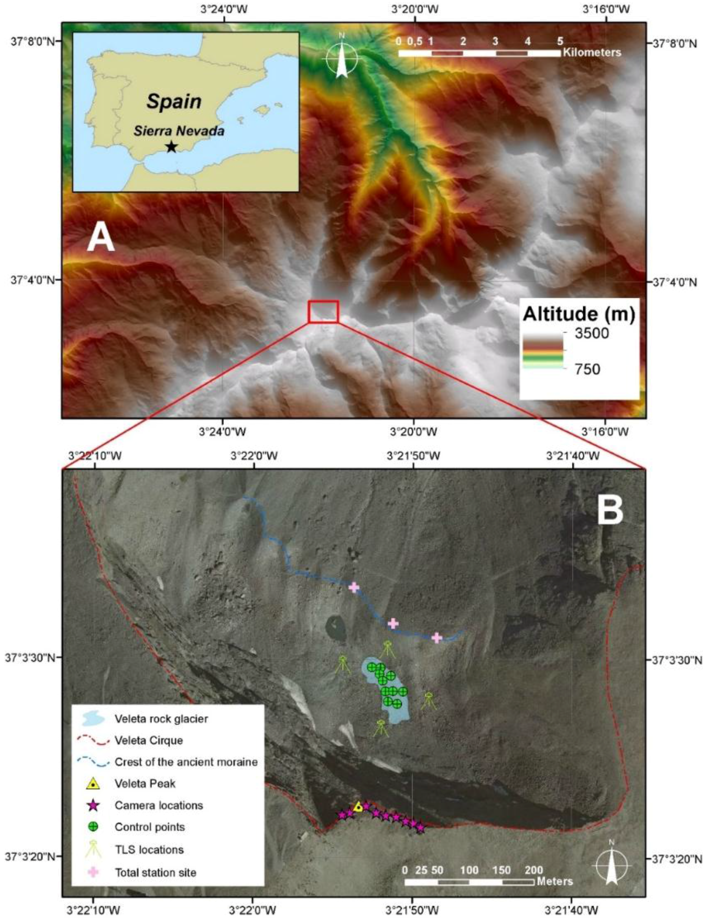
27] suggest that accuracies around 0.1 m can be reached from a 50 m survey range, however, in the case of the Corral del Veleta rock glacier the survey range is imposed by the relief to an approximate distance of 300 m from the Veleta Peak (3398 m.a.s.l.). The capture of oblique photographs at a lower height with an Unmanned Aerial Vehicle (UAV) would be a good option; however, usual weather conditions with variable high-speed gusts of wind make it almost impossible. On the other hand, it is not possible to take ground-based oblique photographs around the glacier because of the highly rough surface covered by blocks that results in large hidden areas from each perspective.
3.2. Average Local Accuracy of Each Point Cloud
Accuracies estimated for every point cloud in a 3D environment using C2C and M3C2 methods varied from 0.084 m to 1.679 m for the point clouds obtained by Agisoft Photoscan and LDR images in 2012 and the point clouds obtained by 123D Catch and HDR images in 2011 (
Table 3). The M3C2 method has been recently proposed as the best way to compare 3D datasets for complex geomorphological features [
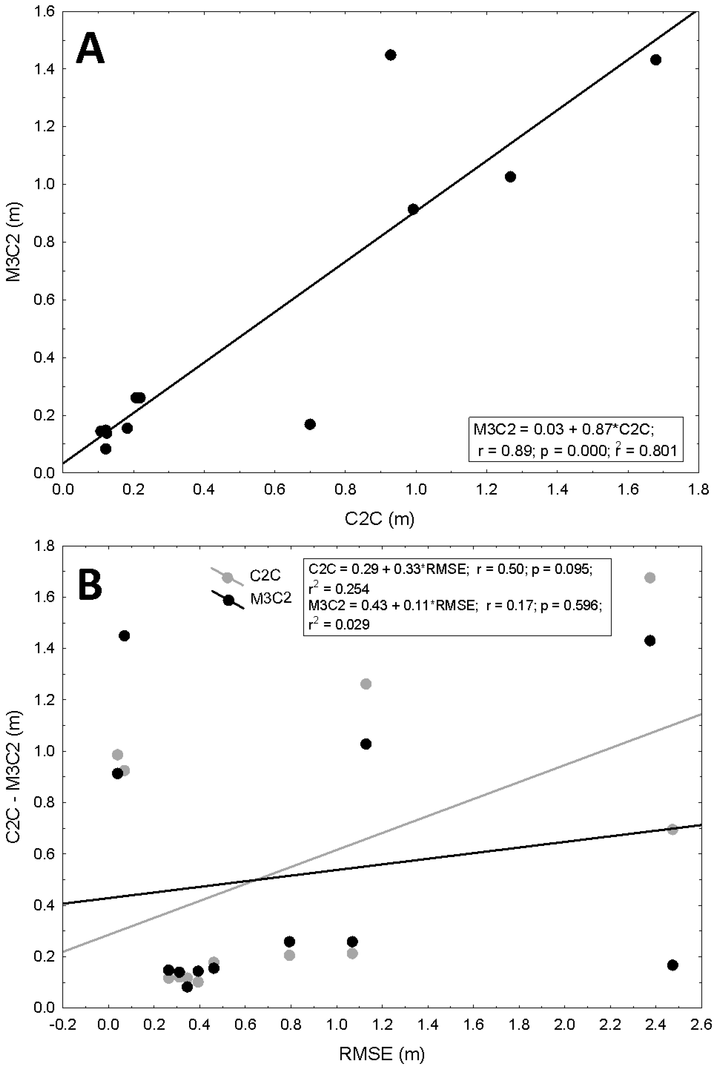
14]. In the present study, M3C2 and C2C presented similar results being correlated with a coefficient R of 0.895 with
p < 0.05 (
Figure 6A). The Corral del Veleta rock glacier presents a special challenge for the C2C algorithm because of the complex and rough surface. Previous works have pointed out that the C2C algorithm is highly sensitive to outliers and the cloud’s roughness [
14]. However, results obtained here showed a similar behavior in the C2C and M3C2 estimations.
On the other hand, the correlation analysis between the 3D more intensive methods (
i.e., estimations based on the analysis of the whole cloud with the C2C and the M3C2) and the RMSE (
Figure 6B) resulted in a coefficient R = 0.504 with
p = 0.095 (correlation between C2C and RMSE) and R = 0.171 with
p = 0.596 (correlation between M3C2 and RMSE). These results point out that although RMSE shows the global quality and fit of the structure of the model it is not necessary related to the average local accuracy of every single point in the cloud. Therefore, the RMSE by itself is not working here as a proper descriptor of the quality of the 3D models like it was showed years ago for 2.5D models within GIS environments (
i.e., DEMs) [
42]. Consequently, an analysis based on both kind of parameters, RMSE and C2C/M3C2, is recommended in order to check the lack of non-linear deformations, to estimate the global quality of the 3D model and to quantify the average local or detailed accuracy of the cloud. It should be noted that SfM-MVS approaches work matching features using their texture and illumination conditions, and control points are, usually, artificial features in the scene that have been marked to be clearly visible in the final model. Therefore, any statistic based on these artificial points may be not actually representing the error in the natural points included in the scene. An optional solution to mitigate this effect is to produce the 3D model first and, identify natural points in the 3D scene that can be measured in the field later [
31].
Figure 6.
Correlation between the Cloud-to-Cloud (C2C) and the Multiscale Model-to-Model (M3C2) (A) and between the C2C and the M3C2 with the RMSE (B).
Figure 6.
Correlation between the Cloud-to-Cloud (C2C) and the Multiscale Model-to-Model (M3C2) (A) and between the C2C and the M3C2 with the RMSE (B).
Alternatively, estimations of the quality of the model designed in a 3D environment (such as C2C and M3C2) are highly recommended against more traditional methods commonly used, that are based on gridding the 3D model and using a DEM of Differences approach (DoD) [
43]. This strategy includes errors added during the gridding of the point cloud that can result in an imprecise estimation of the accuracy. Errors associated with the gridding procedure can be interpolation errors or errors derived from the optimal selection of the Z coordinate. For example, and also in the case of the Corral del Veleta rock glacier, [
10] estimated the average absolute difference between two DEMs in 0.51 m: where the first DEM, was the result of rasterizing a point cloud produced by 123D Catch and the second DEM, worked as benchmark dataset and was obtained rasterizing a point cloud acquired by a TLS. However, the comparison of the two point clouds based on the C2C resulted in an average distance of 0.21 m. Therefore, whether the final aim of the analysis is the quantification of geomorphic change, the approach based on 2.5D surfaces may be estimating inaccurately the threshold to identify the real change. Additionally, some researchers have pointed out the unsuitability of tools currently implemented in GIS software packages to manage large 3D files and point clouds [
5]. Other authors have argued that DEMs are the final product of SfM approaches and the errors estimated using raster-based comparisons are more representative of the real final accuracy [
27].
Table 3.
Average absolute distances (AAD) between each point cloud and the benchmark model (acquired with a Terrestrial Laser Scanner). Distances were estimated by means of the Cloud-to-Cloud (C2C) [
41] and the Multiscale Model-to-Model (M3C2) [
14] methods and are presented in meters. Additionally, the median and the 90 percentile (P90) of the AAD for the M3C2 method are presented. Note that the average distances are obtained averaging the value of the C2C or M3C2 for every point in every cloud.
Table 3.
Average absolute distances (AAD) between each point cloud and the benchmark model (acquired with a Terrestrial Laser Scanner). Distances were estimated by means of the Cloud-to-Cloud (C2C) [41] and the Multiscale Model-to-Model (M3C2) [14] methods and are presented in meters. Additionally, the median and the 90 percentile (P90) of the AAD for the M3C2 method are presented. Note that the average distances are obtained averaging the value of the C2C or M3C2 for every point in every cloud.
| | Low Dynamic Range | High Dynamic Range |
|---|
| 123D Catch | Agisoft Photoscan | 123D Catch | Agisoft Photoscan |
|---|
| 2011 | -C2C (AAD, meters) | 1.266 | 0.990 | 1.679 | 0.926 |
| -M3C2 (AAD, meters) | 1.029 | 0.916 | 1.432 | 1.451 |
| -M3C2 median (meters) | 0.705 | 0.391 | 0.771 | 0.306 |
| -M3C2 P90 (meters) | 2.327 | 2.551 | 3.745 | 3.551 |
| 2012 | -C2C (AAD, meters) | 0.180 | 0.121 | 0.697 | 0.123 |
| -M3C2 (AAD, meters) | 0.157 | 0.084 | 0.171 | 0.141 |
| -M3C2 median (meters) | 0.114 | 0.072 | 0.071 | 0.067 |
| -M3C2 P90 (meters) | 0.345 | 0.222 | 0.277 | 0.217 |
| 2014 | -C2C (AAD, meters) | 0.207 | 0.119 | 0.217 | 0.105 |
| -M3C2 (AAD, meters) | 0.261 | 0.151 | 0.261 | 0.147 |
| -M3C2 median (meters) | 0.180 | 0.086 | 0.183 | 0.079 |
| -M3C2 P90 (meters) | 0.553 | 0.291 | 0.743 | 0.253 |
The geometry of the camera pose during the capture has been pointed out as the source of systematic errors in 3D models obtained by means of SfM-MVS techniques [
44]. This is especially evident in the case of photographs acquired by Unmanned Aerial Vehicles (UAV), which produced multi-image networks with near parallel viewing directions [
44] resulting in dome-type systematic errors. In the previous section, it was hypothesized that the global accuracy of the models could be notably improved using a convergent geometry during the capture according to the differences between the average survey range figures estimated for geomorphological features [
27] and the survey range obtained here. The camera network geometry can also influence the existence of systematic errors in the resulting point clouds. In this work, camera locations are highly limited by the relief (
Figure 2 and
Figure 1B) and the existence of systematic errors was evaluated analyzing the spatial distribution of M3C2 distances (
Figure 7) and visualizing gradient maps.
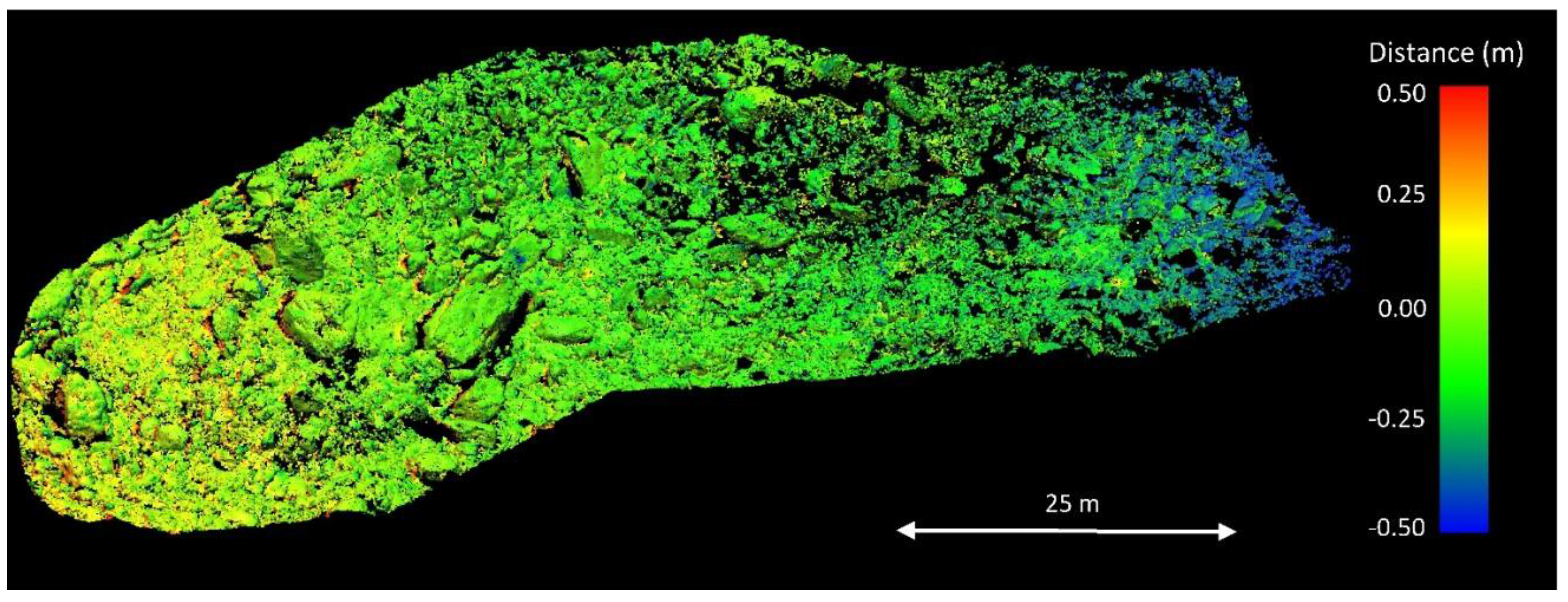
Figure 7 shows the lower distances between the TLS benchmark model and the point cloud produced by Agisoft Photoscan with LDR images for the year 2014 (
i.e., <−0.40) in the head of the glacier which is located in the limits of the study area and is the unique zone in 2014 that presents a thin film of snow. Probably, this fact is due to the presence of the small remain of snow because no other border effects or dome-type errors were found. Regarding the highest positives distances (
i.e., >0.40) they are usually located in hidden areas under debris blocks that are not clearly visible in all the photographs. Therefore, no systematic error was found in the 3D models with this approach.
Figure 7.
Three dimensional view of the spatial distribution of the Multiscale Model-to-Model (M3C2) distances between the benchmark Terrestrial Laser Scanner (TLS) 3D model and the point cloud produced by Agisoft Photoscan with Low Dynamic Range (LDR) images for the year 2014.
Figure 7.
Three dimensional view of the spatial distribution of the Multiscale Model-to-Model (M3C2) distances between the benchmark Terrestrial Laser Scanner (TLS) 3D model and the point cloud produced by Agisoft Photoscan with Low Dynamic Range (LDR) images for the year 2014.
3.3. Comparison between Workflows and Covers
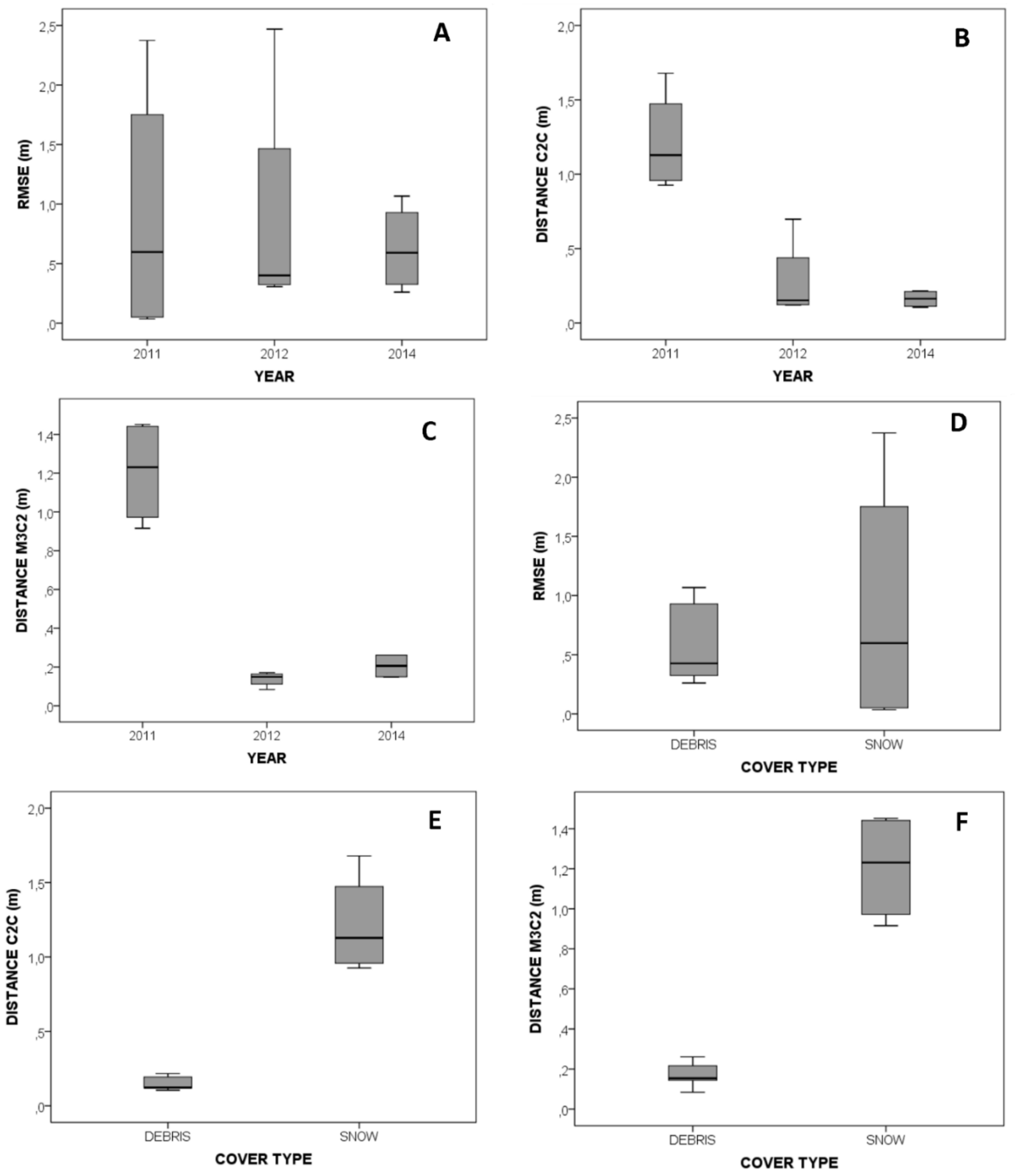
Simple statistical tests and box-whisker plot diagrams were elaborated to allow comparison between the accuracy of the point clouds obtained with different software, procedures and covers (
Figure 8 and
Figure 9) hence instruments and techniques were the same during the study. As stated earlier, in 2011 the whole glacier was covered by a layer of snow (
Figure 5), and therefore, the photographs were quite different from those captured in the years 2012 and 2014. Box-whisker plot diagrams were elaborated using the data from
Table 2 and
Table 3 and grouping the values according to the year of the field survey (
Figure 8A–C) and the cover type of the glacier when the survey was carried out (
Figure 8D–F). The RMSE did not show significant differences between the point clouds grouped by years, however, the analysis of the C2C and M3C2 absolute average distances showed that years 2012 and 2014 resulted in more accurate point clouds as compared to 2011 (
Figure 8B,C). This result is also supported by the residuals of the camera model parameters that presented the higher values for 2011 (
Table 1). During the study, there were not changes in the instruments or the methodological procedures so significant variations in the accuracy of the point clouds are attributed to the changes in the materials covering the glacier. In 2011, the Corral del Veleta was completely covered by a layer of snow while in 2012 and 2014 the debris deposit above the glacier was uncovered. One of the factors determining the accuracy of SfM-MVS methods is the texture of the images used as input. In the case of the year 2011, the photographs presented a poor texture as compared to the debris cover in the photographs of 2012 and 2014. Consequently, more inaccurate point clouds are obtained for snow-covered surfaces (
Figure 7E,F) and this fact should be taken into account when analyzing geomorphic changes with multi-temporal approaches. The possibility of getting poor point clouds in areas covered by snow was already hypothesized by recent works [
5,
31]. Recently, two models of a small glacier partially covered by debris and snow, obtained by means of a TLS and SfM-MVS were compared [
25]. This work concluded that the quality of the SfM-MVS model was, in this specific case, mainly determined by the geometry of the images and camera characteristics [
25]. However, the former analysis was based on the differences of DEMs interpolated using the point clouds and not directly in the 3D model. An alternative to enhance the performance of SfM-MVS in featureless surfaces based on projecting noise function-based patterns in the data collection phase [
45]. This alternative introduces an additional post-processing procedure and should be further explored. On the other hand, the stability of the RMSE over the years and with different covers is due to the fact that the flags used to mark the locations of control points look similar in the photographs independently of the cover over which they were set and the procedure to measure these coordinates over the time was the same. Other recent work [
5] reconstructed the relief of a moraine complex in Nepal and found out the presence of artifacts in an area of the scene largely covered by snow. However, in the case of the Corral del Veleta, areas covered by snow did not showed any artifacts when compared to the TLS point cloud and only a reduction in the accuracy of the clouds was showed by the C2C and M3C2 parameters (
Figure 8E,F).
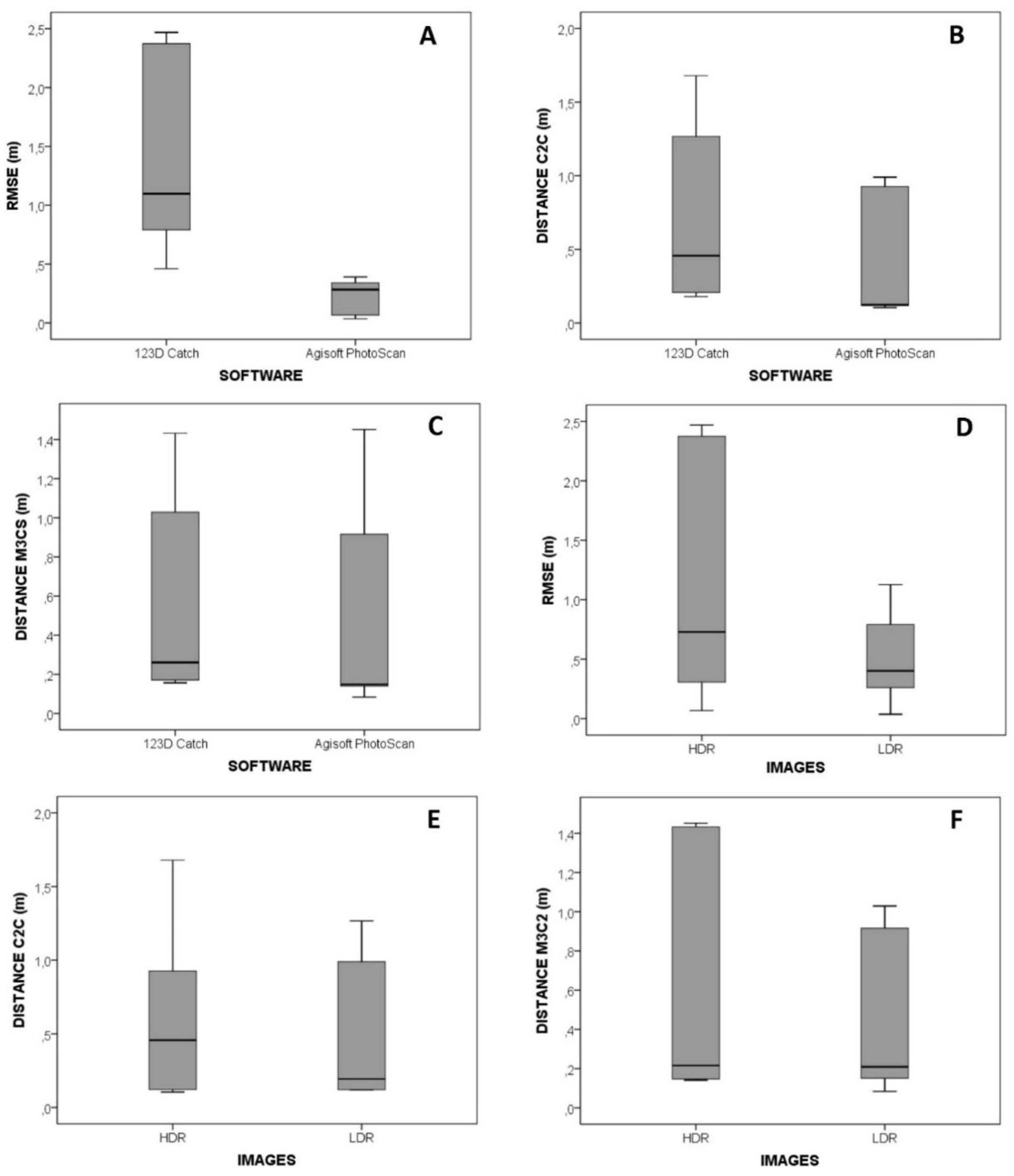
According to the RMSEs estimated in the referencing stage and presented in
Table 2, Agisoft Photoscan software produced more accurate models than 123D Catch software (
Figure 9A). Probably, the bundle adjustment made by Agisoft Photoscan overcomes the procedure developed by 123D Catch software. Additionally, 123D Catch software applies a resolution down-sampling to 3 Mp before processing the images and this effect could be influencing differences observed in
Figure 9A and ahead. However, quantifying the down-sampling effect is not possible while 123D Catch is a free available software but the programming code is not available. In the case of the absolute average distances calculated by the C2C and the M3C2 methods Agisoft Photoscan also always got better results, however these differences were slight and not significant from a statistical viewpoint (
Figure 9B,C).
In general, unprocessed LDR images got the best RMSE, C2C and M3C2 values. Differences between the point clouds feed with HDR compositions and LDR images were non-significant from a statistical viewpoint, although HDR compositions tended to present a higher variability in RMSE (
Figure 9D) and M3C2 distances (
Figure 9F). These results agree with the scarce previous experiences [
33]. In [
33] point clouds of the apse of the Kaisariani Monastery in Greece were produced with Agisoft Photoscan using as input LDR and HDR tone-mapped images. The resulting photo-reconstructions were compared and authors concluded that, from a geometrical viewpoint, the differences between both point clouds were insignificant. However, they just compared the point clouds among them and did not use a benchmark 3D model to estimate the real magnitude of the differences. Previously, [
46] explored the use of HDR images in conventional terrestrial photogrammetry concluding that HDR images resulted in orthophotomosaics with geometrical reliability and a higher dynamic range. In [
32], authors compared the number of points matched using SfM-MVS techniques and HDR-LDR compositions to produce 3D models of cultural heritage objects. [
32] concluded that HDR compositions yielded from 5% to 63% more points matched than LDR images, however differences in the geometrical accuracy of the clouds was not test in this work. In the present work, the amount of points matched within Agisoft Photoscan using HDR pre-processing was slightly higher than the points matched using LDR photographs, producing from 0 to 3% more points matched. In the case of 123D Catch, differences were higher, especially for the year 2011 when 121,758 points matched were obtained using HDR compositions as input as compared to the 89,308 points matched using LDR images. In spite of this increase in the number of points matched, an increase in the geometrical accuracy of the point cloud was not show by the C2C and the M3C2 parameters.
Figure 8.
Box plot diagrams elaborated using the datasets showed in
Table 2 and
Table 3 and grouping these values according to the year of the capture and the cover type. The figure shows the (
A) Root Mean Square Error (RMSE) obtained during the referencing procedure and grouped by year, (
B) absolute average distance from the point clouds to the benchmark model estimated by the Cloud to Cloud (C2C) method and grouped by year, (
C) absolute average distance from the point clouds to the benchmark model estimated by the Multiscale Model to Model (M3C2) method and grouped by year, (
D) RMSE obtained during the referencing procedure and grouped by cover type, (
E) absolute average distance from the point clouds the benchmark model estimated by the C2C method and grouped by cover type and (
F) absolute average distance from the point clouds to the benchmark model estimated by the M3C2 method and grouped by cover type. Note that box plot diagrams show the maximum and the minimum values using the whiskers (upper and lower respectively), the interquartile range (the box) and the median (the line within the box).
![Remotesensing 07 10269 g008]()
Figure 9.
Box plot diagrams showing the (A) Root Mean Square Errors (RMSE) obtained during the referencing procedure and grouped by the software used for the photo-reconstruction (B) absolute average distance from the point clouds to the benchmark model estimated by the Cloud to Cloud (C2C) method and grouped by the software used for the photo-reconstruction, (C) Absolute average distance from the point clouds to the benchmark model estimated by the Multiscale Model to Model (M3C2) method and grouped by the software used for the photo-reconstruction, (D) RMSE obtained during the referencing procedure and grouped by the type of images used in the photo-reconstruction, (E) absolute average distance from the point clouds to the benchmark model estimated by the C2C method and grouped by the type of images used in the photo-reconstruction, and (F) absolute average distance from the point clouds to the benchmark model estimated by the M3C2 method and grouped by the type of images used in the photo-reconstruction. Note that box plot diagrams show the maximum and the minimum values using the whiskers (upper and lower respectively), the interquartile range (the box) and the median (the line within the box).
![Remotesensing 07 10269 g009]()
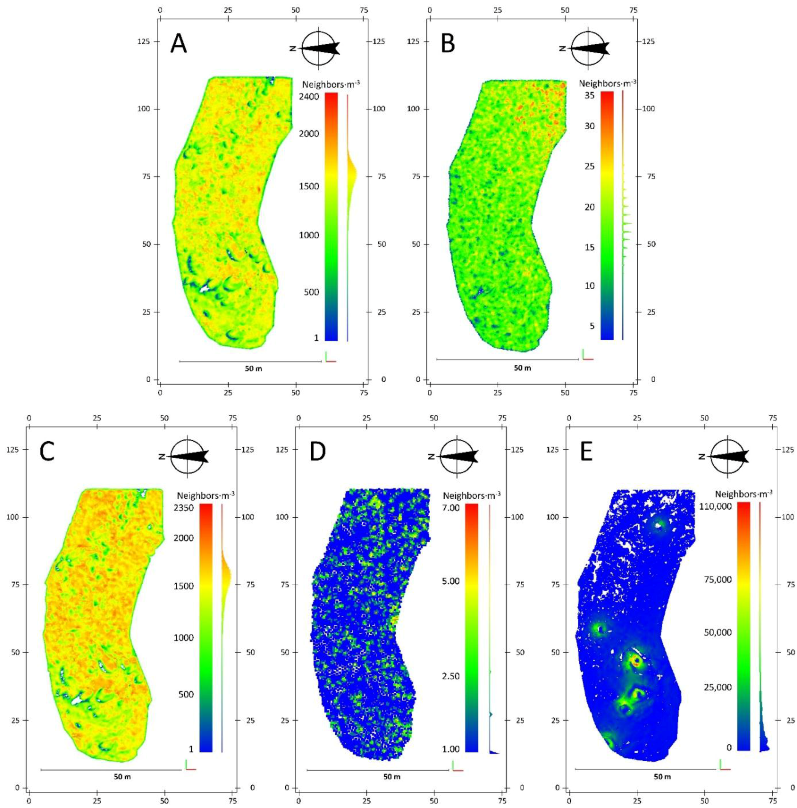
Figure 10.
Volumetric point density for the point clouds of the year 2014 and obtained with (A) Agisoft Photoscan using Low Dynamic Range (LDR) images, (B) 123D Catch using LDR images, (C) Agisoft Photoscan using High Dynamic Range (HDR) compositions, (D) 123D Catch using HDR compositions and (E) the Terrestrial Laser Scanner.
Due to the nature of 3D point clouds obtained by SfM-MVS techniques, their accuracy is commonly linked to point density. So far, most of the approaches in the literature to estimate point density were carried out gridding the space in two dimensions, projecting the location of points over this surface and accounting the number of points in each cell divided by the cell area. These kinds of approaches could experience unreal estimations in complex and rough reliefs like rock glaciers, riverbanks, gullies,
etc. Here, we estimated the volumetric point density,
i.e., from each 3D location, a sphere with a volume of 1 m
3 (
i.e., with a radius of 0.62 m) is defined and the number of points within this volume is accounted.
Figure 10 shows the spatial distribution of point densities for each cloud in 2014. Important differences were observed in the median point density for the clouds generated within 123D Catch. With this software, photo-reconstructions elaborated using LDR images presented point densities an order of magnitude higher than those generated using HDR images, with median values of 20 points·m
−3 and 0.89 points·m
−3, respectively. These results indicate that HDR compositions are not the best input for producing 3D models using 123D Catch software. The exact routine of the matching algorithm used by 123D Catch software is unknown but its performance is clearly affected by the modifications introduced in the HDR compositions, resulting in a lower point density. At the same time, point clouds generated by 123D Catch software presented lower volumetric point densities than point clouds generated by Agisoft Photoscan: 1597 points·m
−3 and 1601 points·m
−3 using LDR and HDR compositions respectively. This lower point density is probably related to the down-sampling to 3 Mp applied by 123D Catch software before matching the images. Volumetric point densities estimated for the point cloud obtained by means of the TLS device presented the highest value with a median of 12,025 points·m
−3.
Finally, an estimation of geomorphic change in the glacier during the study period was not possible because accuracies estimated by the RMSE, the C2C and the M3C2 distances were higher than annual creep velocities and surface lowering of the glacier observed previously [
47].
4. Conclusions
In this study, different workflows were tested in order to produce 3D models of the Corral del Veleta rock glacier for three different years and using SfM-MVS techniques. Two different kinds of images were used as input: conventional Low Dynamic Range photographs (LDR) and pre-processed High Dynamic Range (HDR) compositions. At the same time, two software packages (123D Catch and Agisoft Photoscan) were tested and fed with the LDR images and the HDR compositions.
The RMSEs calculated during the referencing and scaling procedures resulted in a global estimated accuracy that ranged from 0.036 to 2.469 m and the M3C2 mean error ranged from 0.084 (standard deviation of 0.403 m) to 1.451 m (standard deviation of 1.625 m). Values of the RMSE presented here contribute to increase the current knowledge about the performance of SfM-MVS techniques over a wide range of scales and landforms and agree (in magnitude) with other previously presented in the literature. Other two parameters, estimated over the whole point cloud were used to analyze the accuracy of the different SfM-MVS pipelines: the Cloud-to-Cloud method (C2C) and the Multiscale Model-to-Model comparison (M3C2). These methods have been proposed recently as the more suitable approaches to estimate the accuracy of 3D models and point clouds. The M3C2 and the C2C parameters presented a similar performance for the 12 analyzed point clouds. However, important differences were observed when comparing the behavior of the M3C2-C2C and the RMSE, suggesting that the later does not reflect totally the accuracy of the point cloud. Consequently, authors suggest the simultaneous use of the RMSE and the M3C2/C2C for future applications. The values of the RMSE, the M3C2 and the C2C showed that the current methodology could be only applied to estimate relatively large changes in the case of the Corral del Veleta rock glacier (>0.30 m) at medium-term time-scale (5 to 10 years).
Probably, the final accuracy obtained here could be improved using a denser network of oblique camera locations, which in this study are highly constrained by the relief to a few sites. It can be interesting to provide estimations on the accuracy of the models obtained with topographic constraints, as this is the usual situation in high mountain areas. The comparison of the standard parameter survey range (also known as relative precision ratio) showed that the accuracy obtained in this work could be notably improved with a convergent and denser camera network geometry, from 1:370 to approximately 1:639, which is the average value for geomorphological features showed by the literature. The spatial distribution of M3C2 and C2C distances did not show any systematic dome-type error due to the geometry of the pose in the study area.
Having into account the different pipelines, the best performance was produced by Agisoft Photoscan software and LDR images. In fact, no significant improvement was experienced using HDR compositions as input in SfM-MVS methods. At the same time, Agisoft Photoscan overcome 123D Catch, producing more accurate and denser point clouds in 11 out 12 cases.
Regarding the relationship between the cover type and the accuracy, the C2C and the M3C2 parameters showed that years without snow cover (2012 and 2014) resulted in more accurate point clouds as compared to 2011, when the rock debris was covered by snow. However, this difference was not appreciated analyzing the values of the RMSE. It seems logical because the RMSE was estimated for artificial points introduced in the scene. Therefore, those researchers who wish to estimate thresholds of geomorphic change based on the accuracy of the 3D model should have into account that the use of the RMSE may be an erroneous strategy.
Findings presented in this work may be of interest for researchers who want to estimate geomorphic changes using SfM-MVS.


 ,
, 


