Article

Improving the Accuracy of the Water Surface Cover Type in the 30 m FROM-GLC Product

1
Ministry of Education Key Laboratory for Earth System Modelling, Centre for Earth System Science, Tsinghua University, Beijing 100084, China
2
Joint Center for Global Change Studies, Beijing 100875, China
3
Key Laboratory of Technology in Geo-Spatial information Processing and Application System, Institute of Electronics, Chinese Academy of Sciences, Beijing 100190, China
*
Author to whom correspondence should be addressed.
These authors contributed equally to this work.
Remote Sens. 2015, 7(10), 13507-13527; https://0-doi-org.brum.beds.ac.uk/10.3390/rs71013507
Submission received: 3 June 2015 / Revised: 8 October 2015 / Accepted: 13 October 2015 / Published: 16 October 2015

Abstract

:
The finer resolution observation and monitoring of the global land cover (FROM-GLC) product makes it the first 30 m resolution global land cover product from which one can extract a global water mask. However, two major types of misclassification exist with this product due to spectral similarity and spectral mixing. Mountain and cloud shadows are often incorrectly classified as water since they both have very low reflectance, while more water pixels at the boundaries of water bodies tend to be misclassified as land. In this paper, we aim to improve the accuracy of the 30 m FROM-GLC water mask by addressing those two types of errors. For the first, we adopt an object-based method by computing the topographical feature, spectral feature, and geometrical relation with cloud for every water object in the FROM-GLC water mask, and set specific rules to determine whether a water object is misclassified. For the second, we perform a local spectral unmixing using a two-endmember linear mixing model for each pixel falling in the water-land boundary zone that is 8-neighborhood connected to water-land boundary pixels. Those pixels with big enough water fractions are determined as water. The procedure is automatic. Experimental results show that the total area of inland water has been decreased by 15.83% in the new global water mask compared with the FROM-GLC water mask. Specifically, more than 30% of the FROM-GLC water objects have been relabeled as shadows, and nearly 8% of land pixels in the water-land boundary zone have been relabeled as water, whereas, on the contrary, fewer than 2% of water pixels in the same zone have been relabeled as land. As a result, both the user’s accuracy and Kappa coefficient of the new water mask (UA = 88.39%, Kappa = 0.87) have been substantially increased compared with those of the FROM-GLC product (UA = 81.97%, Kappa = 0.81).

Graphical Abstract

1. Introduction

Land surface water cover information is critical to studies such as climate change, flood monitoring and crop yield prediction at the global scale [1,2]. The recent advancement of remote sensing technology makes it possible to have sufficient satellite data that provide continuous coverage of the Earth’s surface with finer spatial resolution and quality. Some of these data have been used to automatically classify global land cover at 30 m resolution [3]. However, the quality of water cover in general purpose land-cover classification using remotely sensed data is often contaminated by cloud shadows and land background of shallow water surfaces. Therefore, it is necessary to improve existing water mask products using alternative approaches.
There exists a number of datasets of global water masks such as the Global Self-consistent Hierarchical, High-resolution Geography (GSHHG) [4], the Global Lakes and Wetlands Database (GLWD) [5], the Shuttle Radar Topography Mission (SRTM) Water Body Detection (SWBD), the Boston University land–sea Mask [6], and the MOD44W [7]. In addition, general purpose global land-cover maps such as IGBP DISCover [8], GLC2000 [9], and GLobCover [10] also contain water layers. The SWBD derived from the SRTM digital elevation model (DEM) has a resolution of 90 m, but it only covers the Earth’s surface between 56°S and 60°N. The MOD44W is a 250 m spatial resolution product derived from the SWBD in combination with the MODIS 250 m data [7]. In summary, except for the 90 m and 250 m products, most of the above global water masks have a resolution coarser than 500 m.
However, as more Landsat-level data become freely accessible, it is natural for researchers to consider adopting these finer resolution data for global mapping [3]. In 2011, the first 30 m resolution global land-cover maps using Landsat Thematic Mapper (TM) and Enhanced Thematic mapper Plus (ETM+) data were developed, and this database is known as the Finer Resolution Observation and Monitoring of Global Land Cover (FROM-GLC) [3]. The images used to produce FROM-GLC were primarily acquired around 2010. In 2014, global water cover maps for two base years, 2000 and 2010 were derived using the Landsat TM and China’s HJ-1 satellite images [11]. However, this product is based on the classification of image segments whose sizes are greater than 4 × 4 pixels in area or 3 pixels in width. Verpoorter et al. developed an approach called the GWEM (GeoCoverTM Water bodies Extraction Method) to produce a circa 2000 GLObal Water Bodies database (GLOWABO) [12,13] from Landsat data. In 2015, Feng et al. produced a global, circa-2000 inland surface water dataset (GIW) using Landsat ETM+ data with a topographic-spectral classification algorithm [14]. In both methods, a Digital Elevation Model (DEM) was used to reduce the misclassification between mountain shadow and water. However, they are pixel-based methods that require a highly precise DEM. If the DEM is not well geo-referenced or has a coarser resolution, some water pixels in mountainous areas will be missed while some other pixels cast by mountain shadows will still be misclassified as water. In addition, the issue of spectral mixing over water boundary areas is usually ignored in existing water extraction procedures.
From the above, it can be seen that the easiest way to obtain a more accurate and more up-to-date global surface water mask is to refine the FROM-GLC that employed circa 2010 satellite data. This is the objective of this paper. FROM-GLC includes 11 level 1 classes and 29 level 2 classes. Among them, water body is a level 1 class that encompasses four level 2 sub-categories, the lake (61), reservoir/pond (62), river (63) and ocean (64). Four classifiers were employed, including the maximum likelihood classifier (MLC), J4.8 decision tree classifier, Random Forest (RF) classifier and support vector machine (SVM) classifier [3]. Among these four, SVM produced the highest overall classification accuracy. In this article, we will focus on the water mask produced by the SVM.
Table 1. Details of the problems in FROM-GLC water mask.
DescriptionLocationAcquisition Date/Image SizeTM ImageFROM-GLC Image
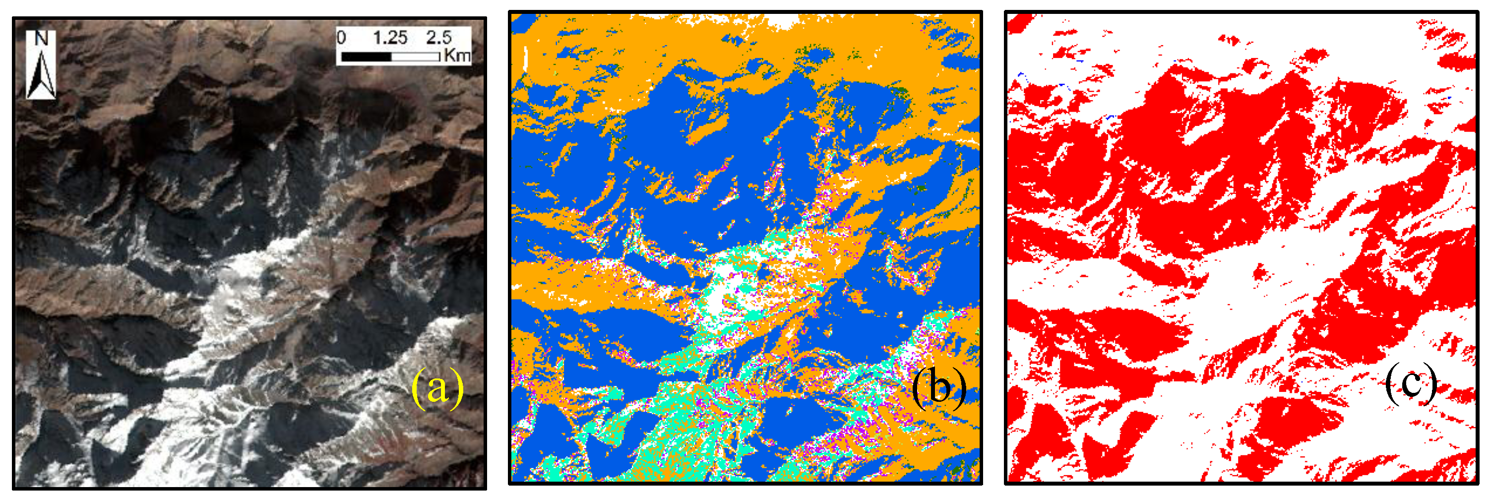
Problem 1:
Commission errors in the mountain shadow area
Alaska,
USA,
North America.
Lat: 62.66°
Lon: −152.16°
Date:
27 September 2011
Size:
400 × 400
Remotesensing 07 13507 i001 Remotesensing 07 13507 i002
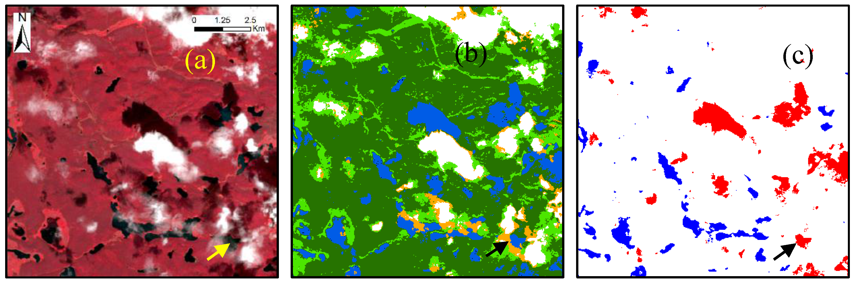
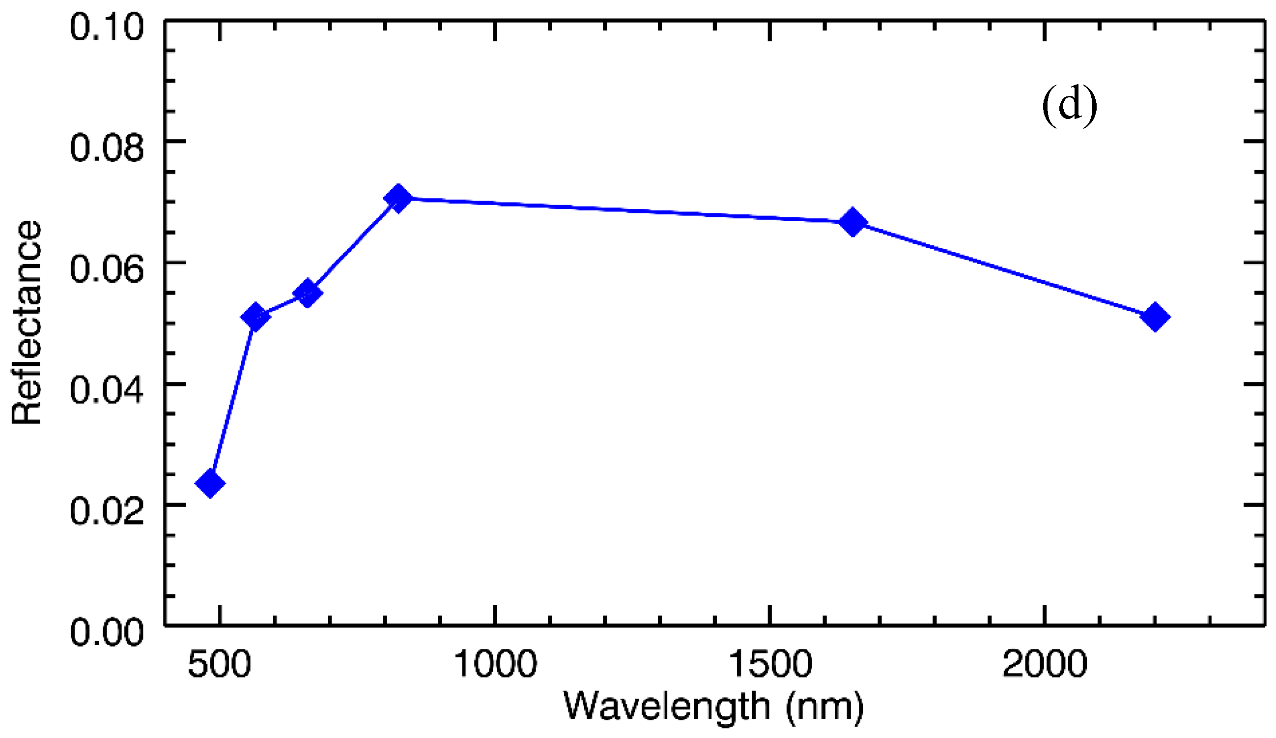
Problem 2:
Commission errors in the cloud shadow area
Maluku, Indonesia, Asia.
Lat: −3.03°
Lon: 128.72°
Date:
30 January 2008
Size:
400 × 400
Remotesensing 07 13507 i003 Remotesensing 07 13507 i004
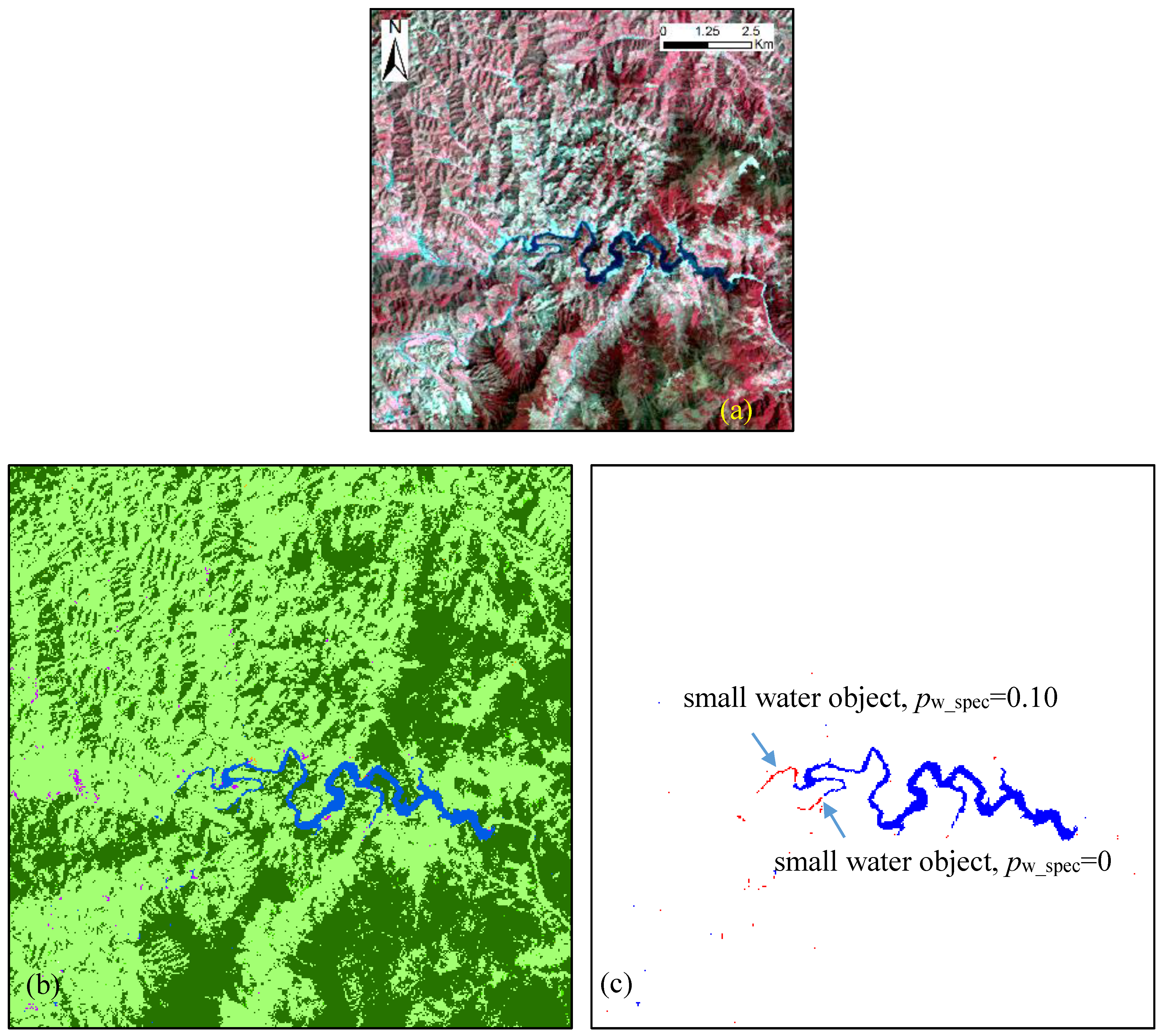
Problem 3:
Spectral mixing at the boundary area
Itapua, Paraguay,
South America.
Lat: −27.36°
Lon: −56.32°
Date:
7 February 2010
Size:
50 × 50
Remotesensing 07 13507 i005 Remotesensing 07 13507 i006
FROM-GLC legend:
Remotesensing 07 13507 i007 Cropland  Remotesensing 07 13507 i008 Forest  Remotesensing 07 13507 i009 Grass  Remotesensing 07 13507 i010 Shrub  Remotesensing 07 13507 i011 Water  Remotesensing 07 13507 i012 Impervious  Remotesensing 07 13507 i013 Bareland 
Remotesensing 07 13507 i014 Snow/Ice  Remotesensing 07 13507 i015 Cloud
When looking deeply into the FROM-GLC water mask, we find that three major problems exist (Table 1): (1) The SVM mistakenly classifies mountain shadows as water. Although topographic correction was performed for more than 6700 scenes with SRTM DEM, some topographic effects in steep mountain regions may still exist. Moreover, since SRTM DEM only covers the Earth’s surface between 56°S and 60°N, more than 1600 scenes located at higher latitudes have not undergone topographical correction. In addition, due to the inconsistent formats, 519 scenes over China, which were collected from the Chinese Satellite Ground Station, have not undergone topographical correction either. In these images, the reflectance of mountain shadow is much lower than the reflectance of the rest of the land area. As a result, mountain shadows are easily misclassified as water by the SVM. (2) Cloud shadows are also easily misclassified as water. Based on FROM-GLC results, more than 95% of the images have clouds, although only 0.81% of the scenes have more than 30% of cloud cover. Similar to mountain shadows, cloud shadows may be classified as water by the SVM. (3) The SVM as a hard classifier may fail to deal with the spectral mixing problem in water-land mixing areas. Therefore, in this article, we report our efforts to solve these three problems in the FROM-GLC water mask product, so as to build a more reliable 30 m resolution water mask for future use. It should be noted that since FROM-GLC is a single-date product, our new water mask is also a static water product.

2. Data Preparation

Besides the FROM-GLC product, additional data used for this study include the following:
  • Landsat TM/ETM+ atmosphere corrected data at 30 m resolution for water spectral feature extraction and water fraction calculation. Scenes from 56°S to 60°N except for China have had topographical correction to alleviate the topographical effect;
  • ASTER 30 m elevation data and SRTM 90 m elevation data for slope calculation. The ASTER DEM is used as supplementary data for areas from 60°N to 80°N where SRTM DEM does not cover;
  • A global validation sample set for validation analysis, which contains 37,711 validation sample units, among which 1555 are in the water category. These were initially designed for validating FROM-GLC. However, the dataset has been carefully improved through several rounds of interpretation and verification, supplemented by MODIS enhanced vegetation index (EVI) time series data and high-resolution imagery from Google Earth [15].

3. Method

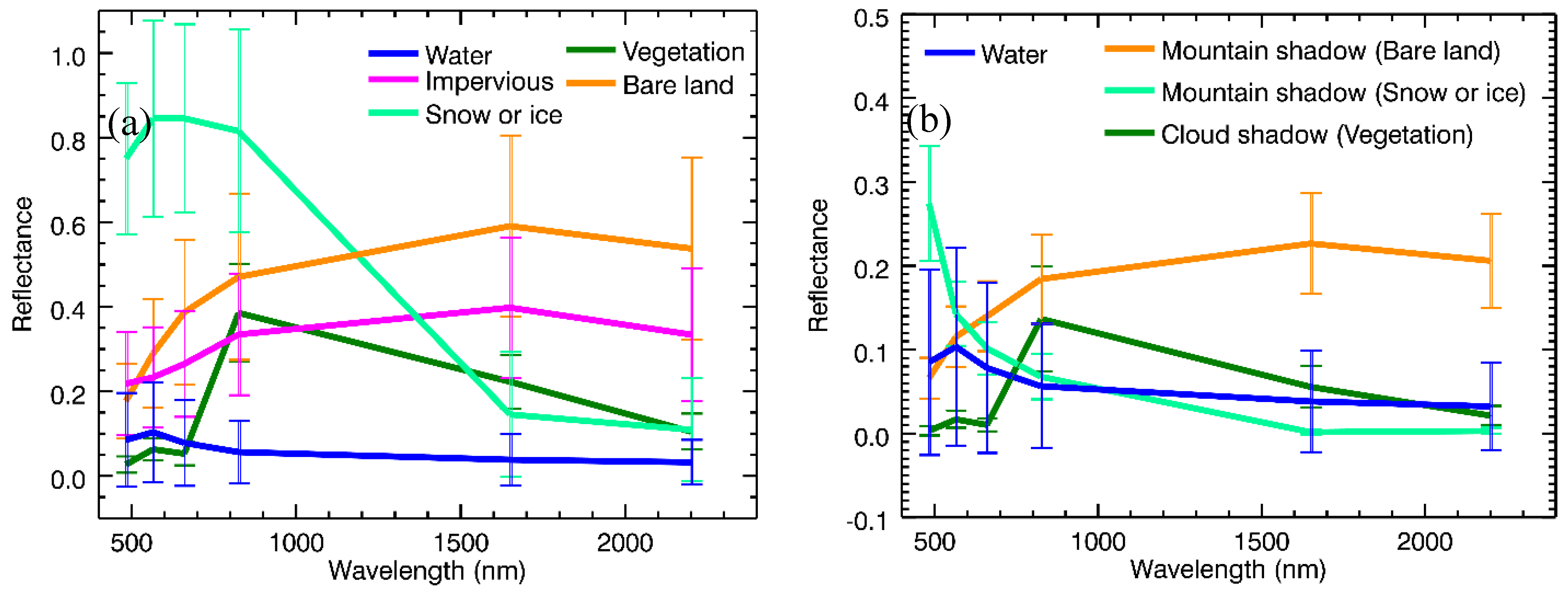
3.1. Spectral and Topographical Characteristics of Water and Land

3.1.1. Spectral Characteristics

According to the global land-cover classification system designed in FROM-GLC, the Earth surface generally consists of vegetation (including crop, forest, grass, and shrub), impervious, bare land, snow/ice and water [3]. One hundred sample units were randomly selected from the validation sample set for each of the five land-cover types [15]. The spectral signatures of the five land-cover types are plotted in Figure 1a. Vegetation has unique spectral features with a green reflectance peak and “red edge” in the visible and near infrared (VNIR) range, while impervious surfaces and bareland follow a fairly flat reflectance pattern, with higher reflectance at the short wave infrared (SWIR) wavelength range. Both snow/ice and water have higher reflectance at the visible (VIS) bands than at the near infrared (NIR) and SWIR ranges. However, the reflectance of snow/ice at VIS is much higher than that of water and other objects, which is why it usually appears bright white in true-color images. Overall, water has the lowest reflectance, especially in the NIR and SWIR bands, where the reflectance of water is close to zero. Therefore, water bodies typically appear dark in the images.
Figure 1. Spectral signatures (mean ± standard deviation) of water, vegetation, impervious, bareland, snow/ice, mountain shadow and cloud shadow. Signatures of each type in (a) were derived from 100 units randomly selected from the validation sample. Signatures for (1) mountain shadow covering bareland, (2) mountain shadow covering snow/ice, and (3) cloud shadow covering vegetation in (b) were each derived from 100 pixels manually selected from Landsat scenes located at (1) path = 155, row = 037, date = 2009.09.06; (2) path = 001, row = 008, date = 2006.7.21, and (3) path = 001, row = 058, date = 2008.09.28, respectively.
Remotesensing 07 13507 g001
The shadows also have a relatively low reflectance as has that of water. In a Landsat image, there are two major types of shadow, mountain and cloud shadow. To show the spectral overlaps between water and shadow, we manually selected 100 pixels on each of three Landsat images for mountain shadows covering bareland and snow/ice, and cloud shadows covering vegetation. The spectral signatures are plotted in Figure 1b. One can find that both water and shadow have very low reflectance in all six bands with strong spectral overlaps (the only exception is for the reflectance of shadow over bareland in the two SWIR bands). As a result, there is a high probability that many classifiers misclassify them as water. As demonstrated in the FROM-GLC water mask, many pixels with mountain and cloud shadows have been incorrectly classified as water.
However, comparing the mean spectra of shadows with those of the corresponding land-cover types in Figure 1a, we can see that shadows can preserve the spectral shapes of the corresponding ground objects. For example, the cloud shadow pixels covering vegetation also have the green peak and “red edge” in the VNIR range. This spectral feature of shadow is helpful to distinguish it from water.

3.1.2. Topographical Characteristics

According to a report on the geographical characteristics of China’s wetland for 2000, wetlands with slopes less than 3° and 8° occupy 93.85% and 99.17% of the total wetland areas, respectively [16]. In this report, wetland includes river, lake, reservoir/pond and urban/entertainment water. That is to say, water bodies are usually distributed on flat terrain. Many researchers have tried to apply topographic slope data to eliminate the shadow at mountainous regions on different types of images [11,17,18]. Typically, they create a slope mask by setting a proper threshold to filter out potential mountain shadows before water mapping. Although the method is simple, their experimental results indicate that it is effective in removing mountain shadows whose spectral characteristics are difficult to distinguish from those of water.
Next, we will first discuss the object-based algorithm for reduction of misclassification between water and shadow. Both spectral and topographical differences between water and shadow are utilized to find out shadows misclassified as waters. Then, a local unmixing method is introduced to solve the spectral mixing problem at the water-land boundary.

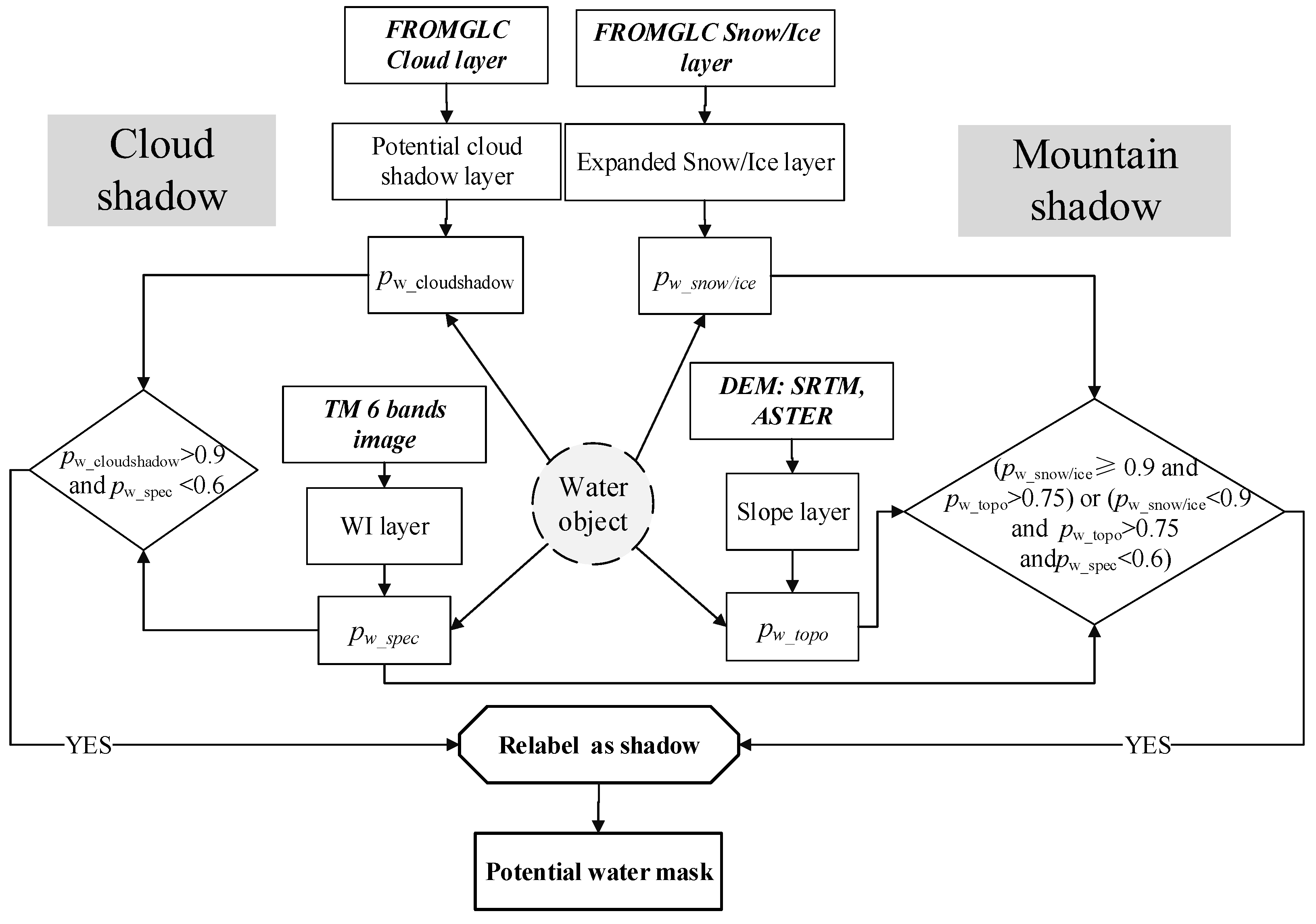
3.2. Object-Based Method to Remove Misclassification in Mountain and Cloud Shadows

3.2.1. Mountain Shadow Object

FROM-GLC is the result of a per-pixel classifier using six bands only, without incorporating any spatial context. However, the water body is usually spatially compact, and pixels within a water body are relatively homogeneous both spectrally and topographically. Thus, water objects are directly extracted from the classification results of FROM-GLC instead of performing image segmentation as done elsewhere [19]. On the other hand, other related objects, such as cloud, snow/ice, and shadow also have similar features. Therefore, in this study, we first adopt the object-based method to improve the accuracy of the FROM-GLC water mask.
The basic idea is that by calculating the spectral and topographical statistics of each water object from the FROM-GLC water mask, and the geometric relationship between a water object with a cloud object, we can identify whether a water object comes from a mountain or cloud shadow. A mountain shadow that is misclassified as water, usually has a greater slope than that of a real water object. Therefore, we can compute the probability of an object located on a mountain slope as follows:
p w _ topo = n w _ topo / N
where N is the total number of pixels in a water object, and nw_topo is the number of pixels with a slope ≥Tw_topo (Tw_topo is a threshold). According to findings in other studies [11,16,17], we set T­w_topo to 8°. However, the SRTM DEM has a coarser spatial resolution (90-m) than FROM-GLC, so some small water bodies in mountainous areas may also have a large pw_topo. As a result, these water objects may be filtered out by the threshold method using pw_topo only. From Figure 1, we can find that the biggest spectral feature of water versus vegetation, impervious and bareland is that it has higher reflectances in the VIS bands than in the NIR and SWIR bands. Therefore, we define a simple water index (WI) by:
WI = { 0 , if max  { band 1 , band 2 , band 3 } max  { band 4 , band 5  band 7 } 1 , if max  { band 1 , band 2 , band 3 } > max  { band 4 , band 5  band 7 }
where band1–5, 7 refer to the 1st–5th, 7th band of the TM/ETM+ image. Compared to other water indices, such as MNDWI [20] and AWEI [21], WI is more straightforward, as it requires no additional threshold parameter, and has lower computational cost. Next, we can construct the probability of an area identified as water in FROM-GLC actually being water using spectral features as follows:
p w _ spec = n w _ spec / N
where nw_spec is the number of pixels with WI = 1. Although some water pixels with vegetation may have WI = 0, most real water objects will have high pw_spec. Mountain shadows, whether covering vegetation or bare land, will have low pw_spec.
However, like other water indices, such as MNDWI and AWEI, WI in Equation (2) is not able to distinguish water from snow/ice [22]. As shown in Figure 1, snow/ice and the mountain shadow pixels covering snow/ice also have higher reflectance in VIS, so their WIs will also be equal to 1. Since the reflectance of mountain shadows covering snow/ice is also low (see Figure 1b), the SVM classifier will misclassify them as water. As a result, the misclassified snow/ice shadow object will also have high pw_spec. Therefore, for misclassified mountain shadows covering snow/ice, pw_spec does not work, and pw_topo is the only effective parameter to distinguish them from water. To judge whether a shadow object is covered by snow/ice, we first dilate the FROM-GLC snow/ice mask with 100 pixels in all directions to generate a potential snow/ice shadow layer. Then, we define another probability to determine whether an object is a snow/ice shadow by
p w _ snow / ice  = n w _ snow / ice  / N
where nw_snow/ice is the number of pixels located in the potential snow/ice shadow area.
Taking these together, if a water object from the FROM-GLC water mask satisfies either of the following conditions, it will be modified as a mountain shadow. The first condition is to remove mountain shadows that cover snow/ice, while the second is to remove those covering bare land or vegetation.
( 1 )   p w _ snow / ice  T snow / ice  and  p w _ topo > T topo  
( 2 )   p w _ snow / ice < T snow / ice  and  p w _ topo > T topo  and  p w _ spec < T spec

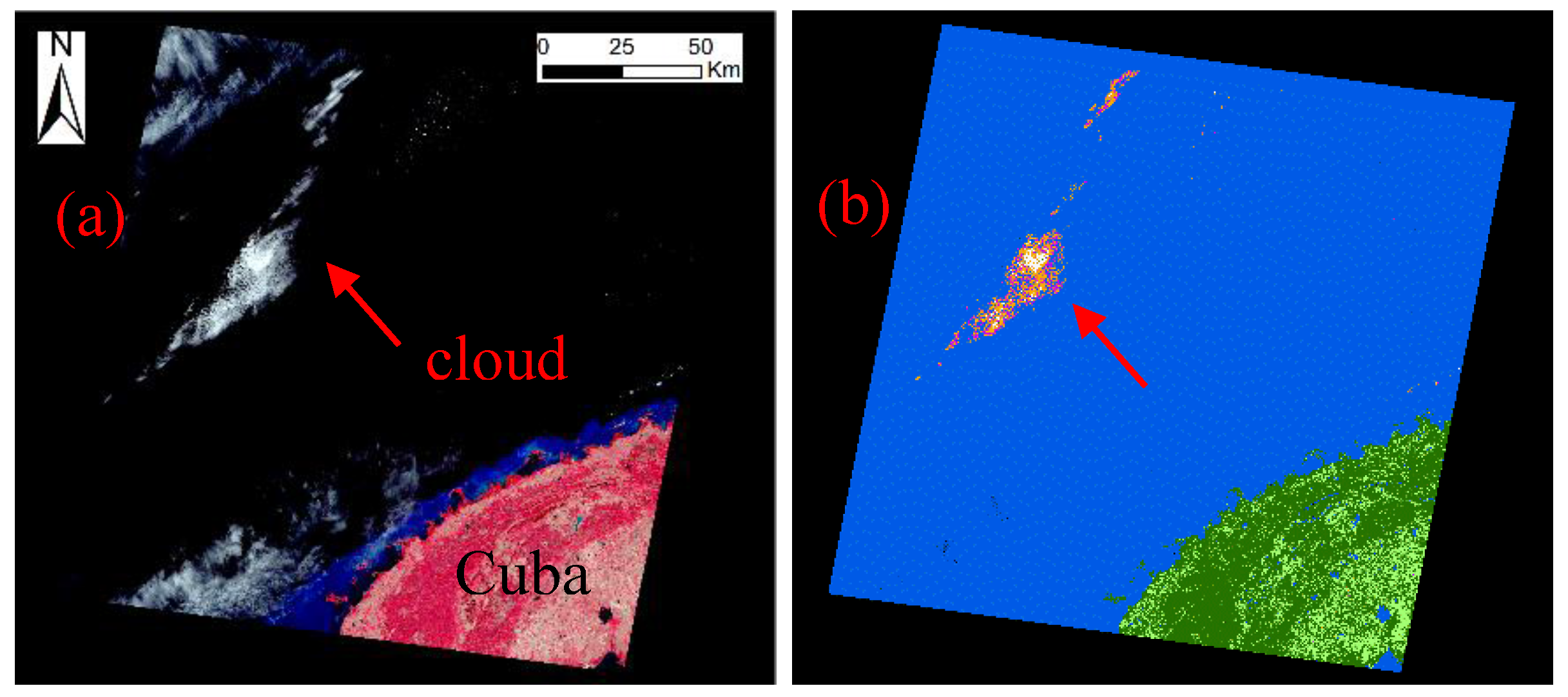
3.2.2. Cloud Shadow Object

Cloud shadow, followed by a cloud object in the FROM-GLC product, is often misclassified as water. One possible way to identify cloud shadow is to predict its location based on its geometric relationship with the cloud as long as the view angle of the satellite sensor, the solar zenith and azimuth angle, and the relative height of the cloud are known. The last parameter, cloud height, is unknown in most cases, and can range from 200–12,000 m [23]. Zhu et al. proposed a method to calculate this parameter by iterating cloud base height from a predicted minimum to maximum height [23]. However, that is time consuming. For simplicity, we first predict the projected direction of the cloud shadow using the view angle of the sensor, the solar zenith and azimuth angle [24]; then, calculate the potential shadow layer by moving the cloud object along a projected direction from 1–100 pixels. This range is empirically determined and can cover most of the cases. All pixels that intersect with the moving cloud object are considered as the potential cloud shadow area. Similarly, we define a probability to determine an object being cloud shadow by
  p w _ cloudshadow   = n w _ cloudshadow  / N
where nw_cloudshadow is the number of pixels located in the potential cloud shadow area. Since the potential cloud shadow area is larger than the actual cloud shadow, some real water bodies may also fall into this area. Therefore, the spectral information is added here to pick out the real cloud shadows in the potential cloud shadow region. Any water object that satisfies the following condition will be relabeled as cloud shadow:
  p w _ cloudshadow   > T cloudshadow  and  p w _ spec < T spec
Ttopo, Tcloudshadow and Tspec, are manually set for all images. By visually comparing FROM-GLC with the Google Earth image for several scenes, we set Ttopo = 0.75, Tspec = 0.6 and Tcloudshadow = 0.9. Details on the object-based method to remove mountain and cloud shadows are shown in Figure 2. The right side shows the steps to remove misclassified mountain shadows while the left shows the steps to remove misclassified cloud shadows. The two results are combined to derive the potential water mask. Next, local unmixing is applied to solve the spectral mixing problem.
Figure 2. Flow chart of object-based method for removing misclassification in mountain and cloud shadow. Water objects are derived from the FROM-GLC water mask.
Remotesensing 07 13507 g002

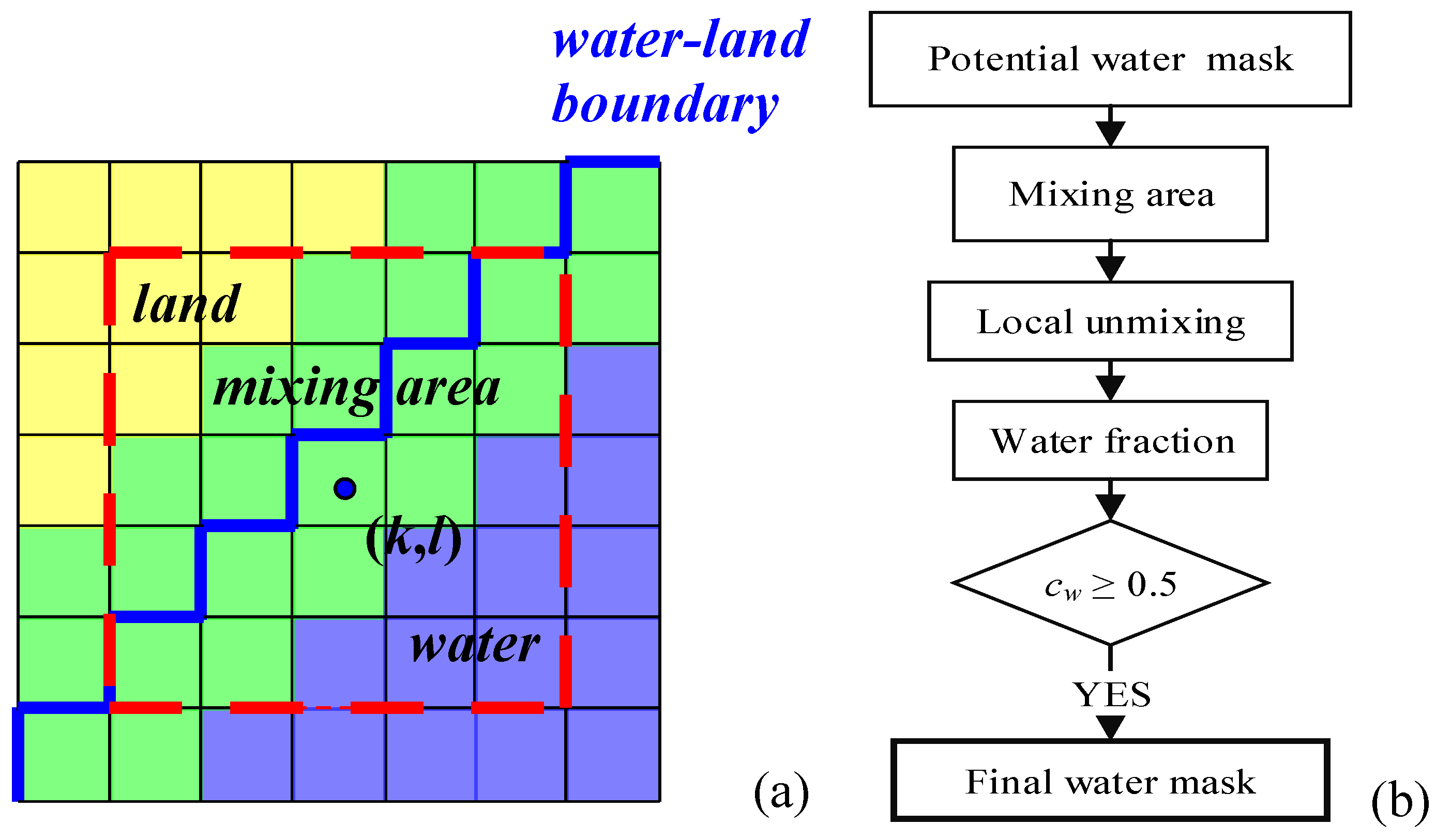
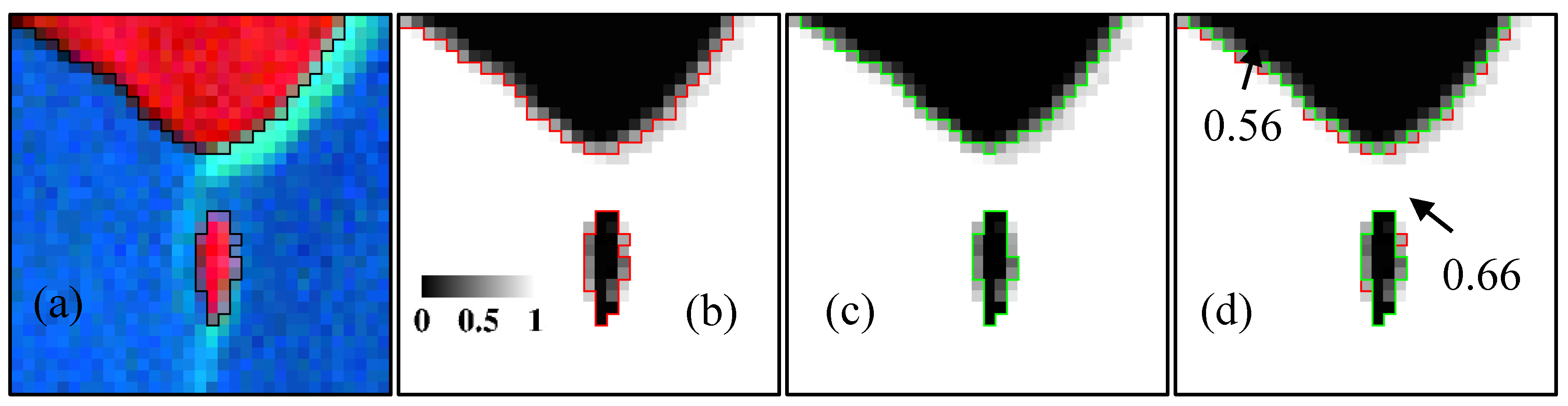
3.3. Solving the Spectral Mixing Problem Using Local Spectral Unmixing

Owing to limited spatial resolution, a large number of mixed pixels exist, especially at the boundaries of different land covers. Many studies show that water bodies are highly dynamic, and a large number of mixed pixels exist, particularly near the water boundaries [25,26,27]. The FROM-GLC water mask is derived from a hard classifier, which assigns each pixel to one of the defined land-cover types. Therefore, water-land mixed pixels exist everywhere along water boundaries in the potential water mask (Figure 2). Here, we reinvestigate the water-land mixing phenomena by soft classification techniques based on fractions of primitive land cover types along the boundary mixed pixels. Their fractions are estimated with a spectral unmixing technique. As illustrated in Figure 3a, a water-land mixing model assumes that a mixed pixel is a linear combination of water and land endmembers weighted by their corresponding fractions, which satisfy the abundance sum-to-one constraint (ASC) and abundance nonnegative constraint (ANC) [28],
r = c w e w + c L e L
c w + c L = 1
c w ,   c L 0
where r is the spectrum of the mixed pixel, eW and eL correspond to the water and land endmembers, and cW and cL represent the fractions of water and land endmembers.
The endmembers can be extracted from the Landsat images using the common endmember extraction algorithms [28,29,30,31,32,33]. However, these algorithms often assume that all pixels in the image are constructed by the same mixing model. Therefore, in most cases, only one water endmember will be extracted. However, different water types may have different optical properties. For example, turbid water generally has higher reflectance in VIS bands [22]. An unmixing error could be introduced if all the water-land mixed pixels use only one water endmember in Equation (9). Therefore, for each mixed pixel, the nearest pure water and land pixels are selected as endmembers. The specific steps are as follows: first, the water-land mixing area in the potential water mask is searched. Here, we define pixels that are 8-neigherhood connected to the water-land boundary as the mixing area (green pixels in Figure 3a). Second, water and land endmembers are searched within a 5 × 5 pixel window. To ensure that water and land endmembers are pure pixels, we select the lowest and the highest reflectance for water and land endmembers, respectively. Next, spectral unmixing is performed with the ASC constraint. Though fully constrained spectral unmixing [34] can obtain fractions strictly in [0,1], it is very time consuming and the local optima problem exists. Thus, we only perform the ASC spectral unmixing in this study. Finally, pixels with a water fraction greater than 50% are labeled as water. Details for the unmixing method are shown in Figure 3b. The procedure follows the object-based analysis in Section 3.2.
Finally, inland water is distinguished from sea water by applying the Global Self-consistent Hierarchical High-resolution Shorelines (GSHHS) [4] version 2.3.4, which is distributed in shapefile format in five different resolutions. The shoreline polygons at full resolution are used here. The algorithm was implemented using the Interactive Digital Languages (IDL). Some procedures that come with the Environment for Visualizing Images (ENVI) software were also utilized, such as the file input/output, map projection conversion, and image mosaicing.
Figure 3. Illustration (a) and flow chat (b) of water local unmixing.
Remotesensing 07 13507 g003

4. Results and Validation

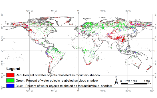
4.1. Results from the Object-Based Method
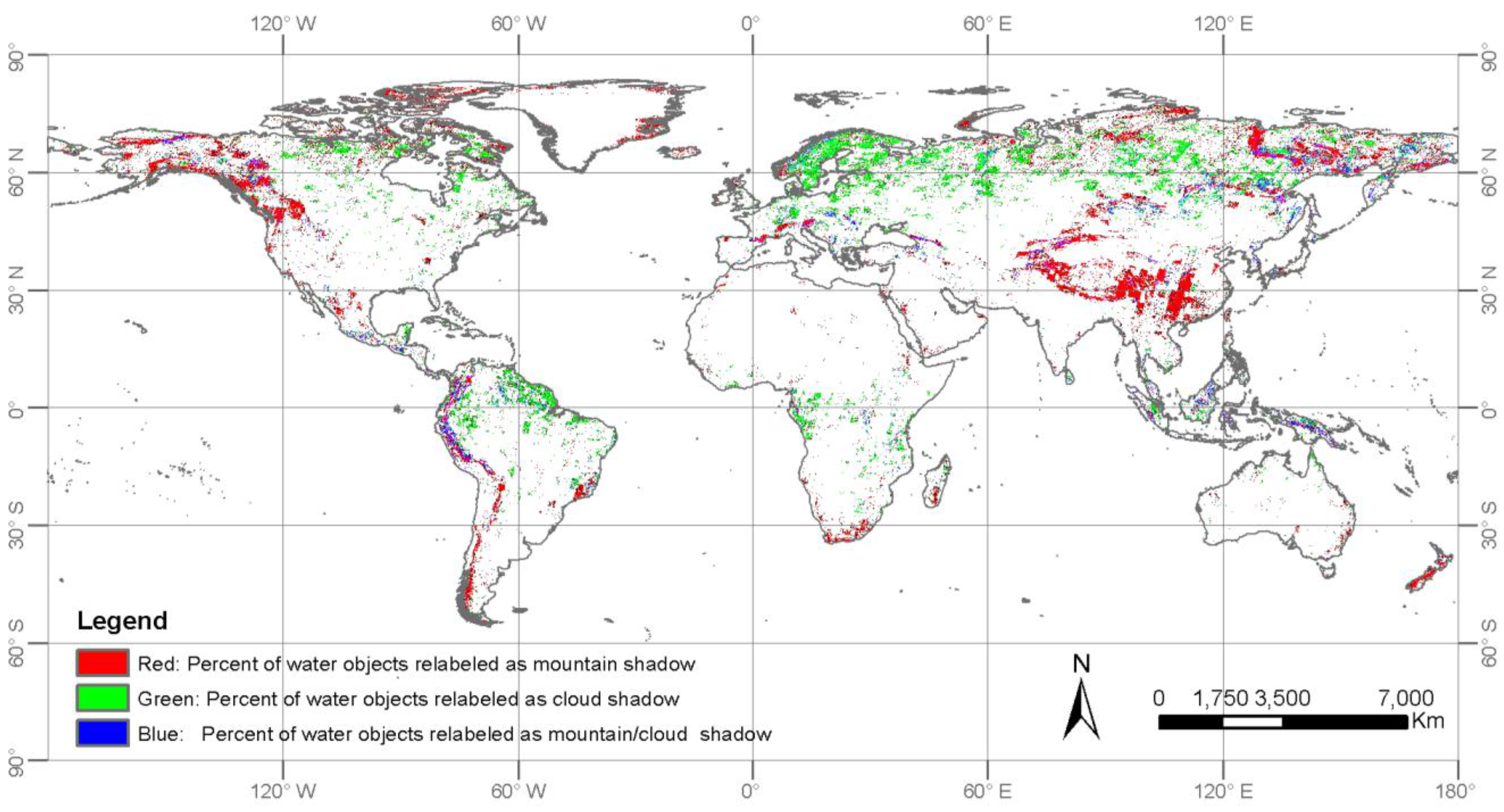
The proposed object-based method is applied to the FROM-GLC water mask to modify the misclassified mountain- or cloud-shadow objects. An example is shown in Figure 4. From the false color image, it can be found that water areas (in blue in Figure 4b) in the FROM-GLC are actually mountain shadows. Since snow/ice exists in this region, Equation (5) is utilized to pick out those misclassified water objects. The result is presented in Figure 4c, where the modified water objects are coloured in red. By utilizing Equation (5), 99.93% of the misclassified water pixels in this area have been corrected.
Figure 4. (a) False color composite image (R: band4, G: band3, B: band2; path: 148, row: 31, date: 23 October 2009); (b) classification result of FROM-GLC (blue: water, cyan: snow/ice); (c) result of the object-based method (red: water object relabeled as mountain shadow).
Remotesensing 07 13507 g004
As mentioned in Section 3.2, owing to the coarse spatial resolution of SRTM, small areas of water between mountains, may also have a high pw_topo. For instance, the pw_topo of the lake in Figure 5 is 0.77, greater than the threshold value for Ttopo. Clearly, this is a snow/ice free region, so if only pw_topoTtopo (0.75) is used, this lake object would be mistakenly marked as mountain shadow. However, the p­w_spec of the lake is 0.62, greater than Tspec (0.6). That is to say, if the spectral constraint condition, pw_specTspec, is added, this lake object will be correctly preserved (Figure 5c). Therefore, to distinguish water from mountain shadow in areas without snow/ice, neither topographical nor spectral constraint conditions should be neglected. However, small water objects cut from the main lake in FROM-GLC, were mistakenly recognized as mountain shadows by our method (Figure 5c). This is because the majority of pixels in these small lakes are spectrally mixed with the neighboring land. Therefore, they have low values of pw_spec, and our method fails in this case.
Similarly, using both spatial and spectral constraints as Equation (8), most cloud shadows that have been incorrectly classified into water in FROM-GLC can be recognized by our method (Figure 6). However, if a lake is covered by aquatic plants or thin cloud, its pixels become mixed, where WI may be 0. For example, the lake marked by an arrow in Figure 6a is covered by thin clouds. The spectral shape in Figure 6d indicates that it contains vegetation. As a result, the pw_spec of this lake is low (=0.02). Our method also fails in this case.
Figure 5. (a) False color composite image (R: band4, G: band3, B: band2; path: 120, row: 39, date: 10 April 2009); (b) classification result of FROM-GLC (blue: water); (c) result of the object-based method (red: water object relabeled as mountain shadow, blue: water object unchanged).
Remotesensing 07 13507 g005
Figure 6. (a) False color composite image (R: band4, G: band3, B: band2; path: 121, row: 16, date: 23 June 2010); (b) classification result of FROM-GLC (blue: water, white: cloud); (c) result of the object-based method (red: water object relabeled as cloud shadow, blue: water object unchanged); (d) spectrum for a pixel in the lake marked by an arrow.
Remotesensing 07 13507 g006aRemotesensing 07 13507 g006b
Next, we compute the percentage of water objects in FROM_GLC being globally modified as mountain and cloud shadows. If a water object only satisfies condition Equation (5) or (6), it is relabeled as mountain shadow, and the corresponding percentage is defined as pW-MS in Equation (12). On the other hand, if the water object only satisfies Equation (8), it is relabeled as cloud shadow, and the percentage is defined as pW-CS in Equation (13). However, mountain shadow and cloud shadow are not mutually exclusive, because clouds can appear in mountainous areas. Therefore, the water object that satisfies both Equations (5) and (8) or both Equations (6) and (8) is relabeled as mountain/cloud shadow, and the percentage is defined as pW-MCS by Equation (14). The result is tabulated in Table 2, and it can be seen that more than a quarter of the global water objects (pW-MS = 25.62%) have been modified to mountain shadows by our method. For clarity, we plot the distribution of these three modifications in Figure 7. It can be seen that most water-to-mountain-shadow modifications happen in China and in the alpine regions and also in high-latitude mountain regions. Images taken in the alpine regions have undergone topographical correction whereas those in China and the high latitude areas have not. Therefore, it can be speculated that topographical correction can be effective to exclude confusion with mountain shadow in water mapping at the sub-alpine regions, but may not work well at the alpine regions. The reason why the topographical correction algorithm fails over alpine regions may be due to the coarser resolution of the DEM data.
Comparatively, the percentage of water objects relabeled as cloud shadow is much smaller. This can be attributed to the fact that when producing FROM-GLC, the authors tried to choose images with as little cloud as possible. From Figure 4, it can be seen that the modifications are mostly located in Russia, Northern European, Northern Canada and Amazon region. 2.51% of water objects have been modified as both mountain and cloud shadows. Except for the case where cloud shadows actually lie on mountain slopes, another possibility is snow/ice on mountain peaks misclassified as clouds in FROM-GLC, as shown in Figure 4b. To sum up, a total of 33.65% of the global water objects have been revised as shadows by our object-based method.
  p w MS = Number of water objects satisfying Equation  ( 5 ) or  ( 6 ) Number of water objects × 100 %
  p w CS = Number of water objects satisfying Equation  ( 8 ) Number of water objects × 100 %
  p w MCS = Number of water objects satisfying both Equations  ( 5 ) and  ( 8 ) or  ( 6 ) and  ( 8 ) Number of water objects × 100 %
Figure 7. Distribution of FROM-GLC water objects relabeled as mountain shadow (red), cloud shadow (green) and mountain/cloud shadow (blue).
Remotesensing 07 13507 g007
Table 2. The percentage of water objects relabeled as mountain, cloud, mountain/cloud shadows.
The Water Objects Relabeled AsPercentage (%)
Mountain shadow, pW-MS25.62%
Cloud shadow, pW-CS5.52%
Mountain/cloud shadow, pW-MCS2.51%
Total33.65%

4.2. Results from Local Spectral Unmixing

After we derive the potentional water layer using the proposed object-based method, local spectral umixing is performed to derive the water fraction at the water-land boundary areas. Unlike the above object-based method, local unmixing is a per-pixel procedure. Since the ANC is not applied, the water fraction may have values that are smaller than 0 or greater than 1. For simplicity, corresponding zero and one forcing are performed to make all water fractions fall into the 0–1 range. FROM-GLC water pixels in the boundary area with fractions smaller than 0.5 will be modified as land, while land pixels with greater than 0.5 water fractions will be modified as water. From Figure 8d, we can see that compared with the FROM-GLC water mask (red line), the new water mask (green line) has expanded the water area by including those mixed pixels with greater water fractions.
Figure 8. (a) False color composite image (R: band4, G: band3, B: band2; path: 224, row: 77, date: 25 May 2002) with the FROM-GLC water layer (black lines), (b) water fraction with FROM-GLC water layer (red lines), (c) water fraction with our result (green lines), and (d) water fractions with both FROM-GLC and our result.
Remotesensing 07 13507 g008
For a comprehensive investigation, we calculate the percentage of relabeled water and land pixels according to Equations (15) and (16), and note them as pW-L and pL-W, respectively. The results are listed in Table 3. Close to 8% of land pixels in water boundary areas have been changed to the water class, while fewer than 2% of water pixels have been changed. These statistical results agree with the example in Figure 8. This may be due to the fact that there are more land training samples than water ones.
  p w L = Number of water pixels relabeled as land Number of water pixels in the mixing area × 100 %
  p L w = Number of land pixels relabeled as water Number of land pixels in the mixing area × 100 %
Table 3. The percentage of water pixels relabeled as land to the total water pixels in water-land mixing areas and the percentage of land pixels relabeled as water to the total land pixels in the same areas.
Percentage
water pixel relabeled as land, pW_L1.70%
land pixel relabeled as water, pL_W7.91%

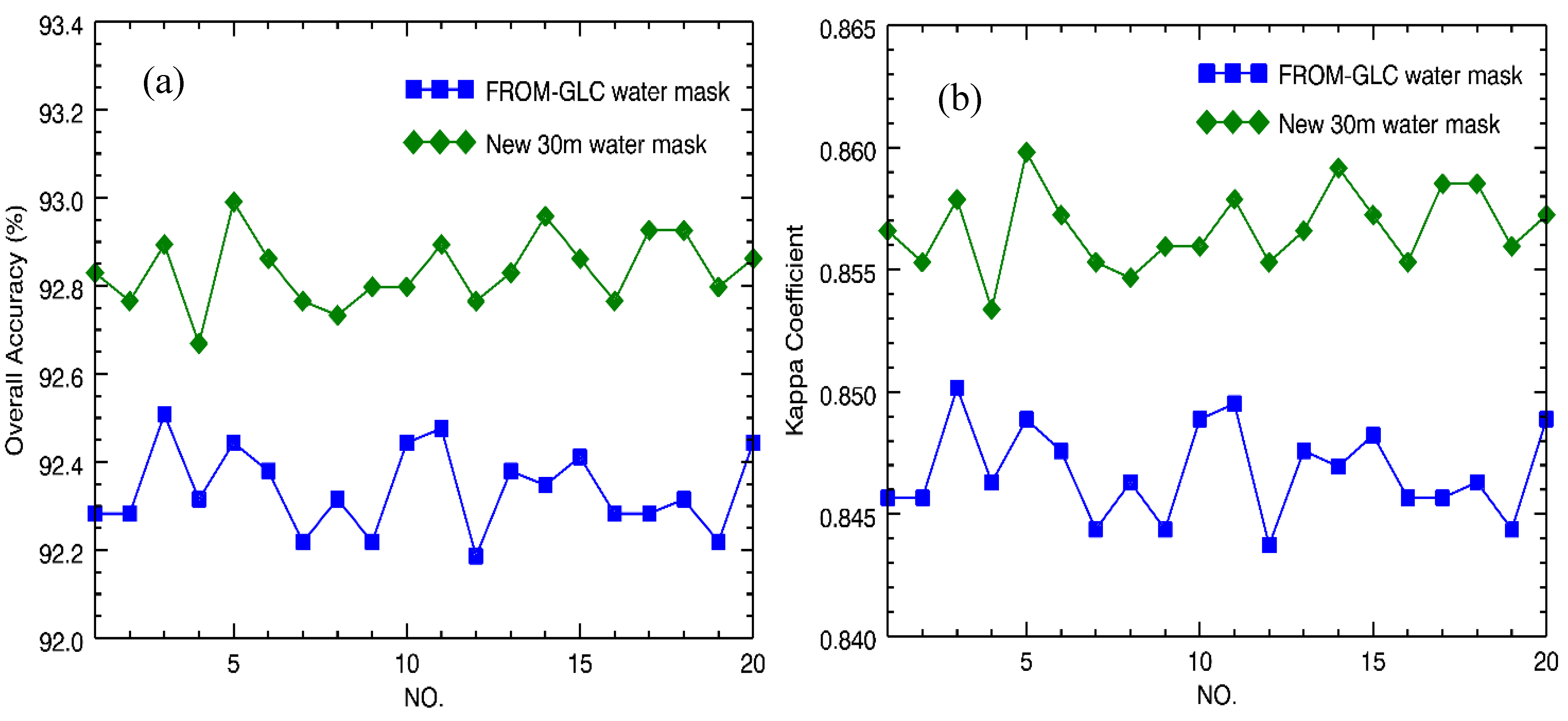
4.3. Validation Using the Global Validation Sample

A global validation data set, with a total of 38,664 sample units, was used to validate the new 30 m water mask. In total, 1555 sample units are water bodies, including lakes, reservoirs/ponds, rivers and offshore ocean [15]. The producer’s accuracy (PA), user’s accuracy (UA), overall accuracy (OA) and Kappa coefficient are calculated for the original FROM-GLC water mask and the new water mask. The confusion matrices are presented in Table 4. After performing the object-based method and local unmixing, all three indices have been raised, especially for the UA. The PA is the probability that true pixels are correctly classified and thus includes only errors of omission, whereas the UA is the probability that classified pixel labels are correct and thus includes only errors of commission [13]. In the FROM-GLC water mask, 293 land sample units were misclassified as water, while in the new water mask, only 173 sample units remain misclassified. This is because most of the mistakenly classified mountain and cloud shadows in the commission errors have been corrected by our method, and thus the UA of the new water mask has been considerably increased, from 81.97%–88.39%. The PA has increased by only 0.51%, which can be attributed to the modification of the misclassified water pixels in water boundary areas. Since only 1.7% of the water pixels have been modified (see Table 3), only eight of the 223 water sample units that were misclassified as land were corrected by the local unmixing method. The Kappa coefficient of our new water mask is 0.87, which is also greater than that of the FROM-GLC water mask (0.81).
Table 4. The accuracy of FROM-GLC and the new 30 m water mask.
FROM-GLCNew 30 m Water Mask
ReferenceReference
LandWaterUA(%)LandWaterUA(%)
ClassificationLand35,86322399.3835,98021599.41
Water293133281.97176134088.39
PA(%)99.1985.6698.6399.5186.1798.96
Figure 9. (a) The overall accuracy, (b) the kappa coefficient of FROM-GLC and the new 30 m water mask when using 1555 water and 1555 randomly selected land sample units after 20 experiments.
Remotesensing 07 13507 g009
In Table 4, it can be seen that the OAs for both water masks are high (the OA for FROM-GLC and the improved water mask is 98.63% and 98.96%, respectively). This is because the size of validation sample for land is much greater than that for water. For a fairer comparison, we randomly selected 1555 land sample units from the total land sample. We then used the 3110 land and water sample units to calculate the overall accuracy and kappa coefficient. This process was repeated 20 times and the results are plotted in Figure 9. It can be seen that the results are very stable when different land sample units are used. The OAs and Kappa coefficient of both water masks have been reduced. However, the new water mask always produces a greater OA (the mean OA for FROM-GLC and the new water mask is 92.34% and 92.83%, respectively). The situation is the same when using the Kappa coefficient as a metric. The new water mask always produces a higher Kappa coefficient (the mean Kappa coefficient of FROM-GLC and the new water mask is 0.847 and 0.857, respectively).

4.4. Overall Distribution of the New Water Mask

Finally, the inland water areas of FROM-GLC and the new water mask for the six continents were estimated. For the overlapping pixels at adjacent Landsat images, the “maximum water area” principle was followed. Though some high-frequency noise may exist as small water objects, we did not perform spatial filtering to remove them. The main reason for this is to keep as many small water bodies as possible.
The new water mask produces a total of 406.86 × 10⁴ km2 of inland surface water in circa-2010. The proportions of all continents are: North America (37.05%), Asia (35.84%), South America (8.77%), Europe (8.53%), Africa (8.53%), and Oceania (1.29%). On the other hand, the FROM-GLC water mask has 483.40 × 10⁴ km2 of total inland water. Comparatively, the inland water area of the new water mask has decreased by 15.83%. This is mainly because 33.65% (see Table 2) of the misclassified shadow objects in the FROM-GLC water mask have been filtered out. From Table 5, we can see that the biggest decrease in water area is in Asia (41.72 × 10⁴ km2), followed by North America (11.0 × 10⁴ km2), South America (9.82 × 10⁴ km2), Europe (8.74 × 10⁴ km2), Africa (3.14 × 10⁴ km2) and Oceania (2.12 × 10⁴ km2). This is in accordance with the spatial distribution of FROM-GLC water objects relabeled as shadow by our method (Figure 7).
When producing the FROM-GLC product, the authors followed a “what you see is what you get” principle to prevent subjective inference of image information from apparent land use [3]. Lakes in tropical and subtropical areas may exhibit totally different cover types ranging from bare land, vegetation, to water surface in different seasons due to large fluctuations of water levels (e.g., Poyang Lake in China [35]). Since only single-date images were used in this study, the new water mask may not be able to capture the maximum water area of those lakes. On the other hand, if a lake or river in a Landsat image is frozen, it will be classified as snow/ice. Therefore, frozen water at the high latitude areas of Asia, Europe and North America may not be included in the new water mask. This issue could be solved by using the multi-temporal data in the future.
Table 5. The water areas for the six continents of FROM-GLC and the new 30 m water mask.
ContinentWater Area (×104 km2)
FROM-GLC Water MaskThe New Water Mask
Asia187.54145.82
Europe43.4334.69
Africa37.8434.70
North America161.73150.73
South America45.5035.68
Oceania7.365.24
Total483.40406.86

5. Discussion

The object-based method proposed in this study is mainly used to reduce the commission errors in the FROM-GLC water mask, which is to exclude mountain and cloud shadows that have been misclassified as water in FROM-GLC. The result is quite promising. Compared with the per-pixel method, the object-based method has a loose requirement for the accuracy of DEM. For instance, small geometrical mismatches between TM images and the DEM will have little influence on the pw_topo of large water bodies. However, this method may lose its advantage when the water object is connected with mountain or cloud shadow in the FROM-GLC water mask [13]. If the water area is smaller than the shadow area, this water body will be mislabeled as shadow by our method. On the contrary, if the water area is larger than the shadow area, the shadow may not be filtered out. One possible way to solve this problem is by initially splitting the water objects in FROM-GLC according to the topographical, spectral or other attributes. However, this may require a series of trials before reaching a satisfactory result. Another possible solution is to perform dynamic water mapping with multi-temporal scenes [25,36,37], because the chances of being covered or shadowed by clouds in multiple images would be significantly lower for certain pixels where the number of cloudy days is small. By fusing multi-temporal images, the cloud issue should be easily overcome for those pixels. However, around the world, many places can be covered by cloud frequently. For those places, our method can be applied in the same way to each single-date image of the multi-temporal dataset. This can exclude the misclassifications between water and shadows, so as to improve the final results. While multi-temporal image analysis focuses more on the process in the time domain, our method concentrates on analyses in the spatial domain.
Though our proposed method is used as a post-classification/detection procedure in this study, it can also be applied directly to the segmentation result in object-based image classification. It should be noted here that the proposed method is not specifically designed to solve the water classification problem in FROM-GLC. The idea presented here can also be employed for other land cover types with obvious spatial characteristics, such as cropland, snow/ice, and cloud.
Local spectral unmixing is used to estimate a reliable water fraction in water boundary areas, so that pixels containing fewer land components are determined as water. This seems to be a more reasonable way. It is an automatic process, and does not require additional inputs. It is not limited to two endmember mixture models, and can be used for other land cover types as well.
Since the image selection criterion when producing FROM-GLC is to select images with the least cloud cover in inland areas during the growing season, the probability of inland water covered by thick cloud is low. That is, the omission error of the inland water is small. Therefore, in this study, we did not do any extra work to exclude cloud covers on inland water. However, cloud distribution on the ocean is not considered when choosing the FROM-GLC images, so the omission error in the ocean regions is much larger. Clouds on the ocean are often misclassified into impervious, bareland or snow/ice, as shown in Figure 10. Some land–ocean masks, such as MOD44W, GSHHG, could be used to filter out the clouds. However, because of geometrical mismatching, the difference in spatial resolution and the difference in image acquisition time, some small islands and shoreline details may be modified incorrectly. Therefore, a method to derive a land-ocean mask for TM/ETM+ image should be the subject of future studies.
Figure 10. (a) False color composite image (R: band4, G: band3, B: band2; path: 17, row: 44, date: 19 December 2000), and (b) the classification result of FROM-GLC (refer to Table 1 for more detailed legend information).
Remotesensing 07 13507 g010
From Table 4, it can be seen that both the PA and UA of our new water mask is greater than 85%, so it can be regarded as a reliable water-land mask for other research. Though it is a single time water mask, it can serve as a base map when studying the temporal change of surface water regionally or globally. Moreover, it can also be used to produce training or validation samples for water mapping or for water fraction derivation from coarser spatial resolution data, such as MODIS images. Using water mapping as an example, the target detection method [22] only requires one input parameter, the spectrum of the target, which can be generated from our new water mask. As a result it is possible to use our water mask for water mapping on TM or coarser resolution images automatically in the future.
In addition, during the course of reducing misclassifications of water, our method created many shadow objects (mountain and cloud shadow) in FROM-GLC. For these shadows, further classification would be needed. Our current method only has the ability to classify shadows into four classes: vegetation, impervious, bare land and snow/ice. However, FROM-GLC includes 11 level 1 classes and 29 level 2 classes. Therefore, well-designed rules are required for further classification. This falls outside the scope of this study.

6. Conclusions

The FROM-GLC water mask is improved by first applying an object-based method to remove the commission errors, and then performing local spectral unmixing at water-land boundary areas. By displaying the locations of FROM-GLC water objects modified as mountain shadow, we found that topographical correction, even when using a coarser resolution DEM, is useful to reduce the confusion between mountain shadows and water bodies, but may fail in high mountain areas. By comparing local unmixing results with FROM-GLC, we found that when the number of training sample units for water is smaller than that for land, some hard classifiers (e.g., SVM) tend to classify the water-land mixed pixels more favorably as land even when the water fraction is greater than that of land.
The new water map has a producer’s and user’s accuracy of 86.17% and 88.39%, respectively. Both are higher when compared with those for the original FROM-GLC (85.66% and 81.97%, respectively). We therefore conclude that the new map has improved the water mask in the FROM-GLC. The new water product is suitable for use in applications that require finer resolution, and can serve as a base map for water mapping with coarser spatial resolution.
However, there still exist some omission errors in water areas covered by clouds. Clearly, the use of multi-temporal images has the potential to remediate the cloud effect. This is our next research target.

Acknowledgments

This research is partially supported by the National Basic Research Program of China (973 Program) under Grant Number 2015CB953701. Furthermore we would like to thank Jie Wang, Kang Jiang and Le Yu for their advice and help. We also thank Yuanyuan Zhao for providing the global validation sample set.

Author Contributions

Luyan Ji: Primary researcher and writer of the research publication; Peng Gong and Xiurui Geng: Technical expertise to the research publication; Yongchao Zhao: Landsat image atmospheric correction software developer and IDL programming advisor.

Conflicts of Interest

The authors declare no conflict of interest.

References

  1. Roberts, N.; Taieb, M.; Barker, P.; Damnati, B.; Icole, M.; Williamson, D. Timing of the Younger Dryas event in East Africa from lake-level changes. Nature 1993, 366, 146–148. [Google Scholar] [CrossRef]
  2. Li, S.; Sun, D.; Yu, Y.; Csiszar, I.; Stefanidis, A.; Goldberg, M.D. A new short-wave infrared (SWIR) method for quantitative water fraction derivation and evaluation with EOS/MODIS and Landsat/TM data. IEEE Trans. Geosci. Remote Sens. 2013, 51, 1852–1862. [Google Scholar] [CrossRef]
  3. Gong, P.; Wang, J.; Yu, L.; Zhao, Y.; Zhao, Y.; Liang, L.; Niu, Z.; Huang, X.; Fu, H.; Liu, S.; et al. Finer resolution observation and monitoring of global land cover: First mapping results with Landsat TM and ETM+ data. Int. J. Remote Sens. 2012, 34, 2607–2654. [Google Scholar] [CrossRef]
  4. Wessel, P.; Smith, W.H.F. A global, self-consistent, hierarchical, high-resolution shoreline database. J. Geophys Res.: Solid Earth 1996, 101, 8741–8743. [Google Scholar] [CrossRef]
  5. Lehner, B.; Döll, P. Development and validation of a global database of lakes, reservoirs and wetlands. J. Hydrol. 2004, 296, 1–22. [Google Scholar] [CrossRef]
  6. Salomon, J.; Hodges, J.C.F.; Friedl, M.; Schaaf, C.; Strahler, A.; Gao, F.; Schneider, A.; Zhang, X.; El Saleous, N.; Wolfe, R.E. Global land-water mask derived from MODIS NADIR BRDF-adjusted reflectances (NBAR) and the MODIS land cover algorithm. In Proceedings of the 2004 IEEE International Geoscience and Remote Sensing Symposium (IGARSS’04), Anchorage, AK, USA, 20–24 September 2004; pp. 239–241.
  7. Carroll, M.L.; Townshend, J.R.; DiMiceli, C.M.; Noojipady, P.; Sohlberg, R.A. A new global raster water mask at 250 m resolution. Int. J. Digit. Earth 2009, 2, 291–308. [Google Scholar] [CrossRef]
  8. Loveland, T.R.; Reed, B.C.; Brown, J.F.; Ohlen, D.O.; Zhu, Z.; Yang, L.; Merchant, J.W. Development of a global land cover characteristics database and IGBP discover from 1 km AVHRR data. Int. J. Remote Sens. 2000, 21, 1303–1330. [Google Scholar] [CrossRef]
  9. Bartholomé, E.; Belward, A.S. GLC2000: A new approach to global land cover mapping from Earth Observation data. Int. J. Remote Sens. 2005, 26, 1959–1977. [Google Scholar] [CrossRef]
  10. Arino, O.; Bicheron, P.; Achard, F.; Latham, J.; Witt, R.; Weber, J.L. GlobCover: The most detailed portrait of Earth. Eur. Space Agency 2008, 136, 25–31. [Google Scholar]
  11. Liao, A.; Chen, L.; Chen, J.; He, C.; Cao, X.; Chen, J.; Peng, S.; Sun, F.; Gong, P. High-resolution remote sensing mapping of global land water. Sci. China Ser. D: Earth Sci. 2014, 57, 2305–2316. [Google Scholar] [CrossRef]
  12. Verpoorter, C.; Kutser, T.; Seekell, D.A.; Tranvik, L.J. A global inventory of lakes based on high-resolution satellite imagery. Geophys. Res. Lett. 2014, 41, GL060641. [Google Scholar] [CrossRef]
  13. Verpoorter, C.; Kutser, T.; Tranvik, L.J. Automated mapping of water bodies using Landsat multispectral data. Limnol. Ocean. Method 2012, 10, 1037–1050. [Google Scholar] [CrossRef]
  14. Feng, M.; Sexton, J.O.; Channan, S.; Townshend, J.R. A global, high-resolution (30-m) inland water body dataset for 2000: First results of a topographic-spectral classification algorithm. Int. J. Digit. Earth 2015. [Google Scholar] [CrossRef]
  15. Zhao, Y.; Gong, P.; Yu, L.; Hu, L.; Li, X.; Li, C.; Zhang, H.; Zheng, Y.; Wang, J.; Zhao, Y.; et al. Towards a common validation sample set for global land-cover mapping. Int. J. Remote Sens. 2014, 35, 4795–4814. [Google Scholar] [CrossRef]
  16. Niu, Z.; Gong, P.; Cheng, X.; Guo, J.; Wang, L.; Huang, H. Geographical characteristics of China’s wetlands derived from remotely sensed data. Sci. China Ser. D: Earth Sci. 2009, 52, 723–738. [Google Scholar] [CrossRef]
  17. Sun, F.; Sun, W.; Chen, J.; Gong, P. Comparison and improvement of methods for identifying waterbodies in remotely sensed imagery. Int. J. Remote Sens. 2012, 33, 6854–6875. [Google Scholar] [CrossRef]
  18. Lu, S.; Wu, B.; Yan, N.; Wang, H. Water body mapping method with HJ-1A/B satellite imagery. Int. J. Appl. Earth Obs. Geoinf. 2011, 13, 428–434. [Google Scholar] [CrossRef]
  19. Blaschke, T. Object based image analysis for remote sensing. ISPRS J. Photogramm. Remote Sens. 2010, 65, 2–16. [Google Scholar] [CrossRef]
  20. Xu, H. Modification of normalised difference water index (NDWI) to enhance open water features in remotely sensed imagery. Int. J. Remote Sens. 2006, 27, 3025–3033. [Google Scholar] [CrossRef]
  21. Feyisa, G.L.; Meilby, H.; Fensholt, R.; Proud, S.R. Automated water extraction index: A new technique for surface water mapping using Landsat imagery. Remote Sens. Environ. 2014, 140, 23–35. [Google Scholar] [CrossRef]
  22. Ji, L.; Geng, X.; Sun, K.; Zhao, Y.; Gong, P. Target detection method for water mapping using Landsat 8 OLI/TIRS imagery. Water 2015, 7, 794–817. [Google Scholar] [CrossRef]
  23. Zhu, Z.; Woodcock, C.E. Object-based cloud and cloud shadow detection in Landsat imagery. Remote Sens. Environ. 2012, 118, 83–94. [Google Scholar] [CrossRef]
  24. Li, S.; Sun, D.; Yu, Y. Automatic cloud-shadow removal from flood/standing water maps using MSG/SEVIRI imagery. Int. J. Remote Sens. 2013, 34, 5487–5502. [Google Scholar] [CrossRef]
  25. Wang, J.; Li, C.; Hu, L.; Zhao, Y.; Huang, H.; Gong, P. Seasonal land cover dynamics in Beijing derived from Landsat 8 data using a spatio-temporal contextual approach. Remote Sens. 2015, 7, 865–881. [Google Scholar] [CrossRef]
  26. Sun, D.; Yu, Y.; Goldberg, M.D. Deriving water fraction and flood maps from Modis images using a decision tree approach. IEEE J. Sel. Top. Appl. Earth Obs. Remote Sens. 2011, 4, 814–825. [Google Scholar] [CrossRef]
  27. Li, S.; Sun, D.; Goldberg, M.; Stefanidis, A. Derivation of 30-m-resolution water maps from TERRA/MODIS and SRTM. Remote Sens. Environ. 2013, 134, 417–430. [Google Scholar] [CrossRef]
  28. Ji, L.; Geng, X.; Sun, K.; Zhao, Y.; Gong, P. Modified N-FINDR endmember extraction algorithm for remote-sensing imagery. Int. J. Remote Sens. 2015, 36, 2148–2162. [Google Scholar] [CrossRef]
  29. Geng, X.; Ji, L.; Zhao, Y.; Wang, F. A new endmember generation algorithm based on a geometric optimization model for hyperspectral images. IEEE Geosci. Remote Sens. Lett. 2013, 10, 811–815. [Google Scholar] [CrossRef]
  30. Berman, M.; Kiiveri, H.; Lagerstrom, R.; Ernst, A.; Dunne, R.; Huntington, J.F. Ice: A statistical approach to identifying endmembers in hyperspectral images. IEEE Trans. Geosci. Remote Sens. 2004, 42, 2085–2095. [Google Scholar] [CrossRef]
  31. Miao, L.; Qi, H. Endmember extraction from highly mixed data using minimum volume constrained nonnegative matrix factorization. IEEE Trans. Geosci. Remote Sens. 2007, 45, 765–777. [Google Scholar] [CrossRef]
  32. Winter, M.E. N-FINDR: An algorithm for fast autonomous spectral end-member determination in hyperspectral data. Proc. SPIE 1999, 3753, 266–275. [Google Scholar]
  33. Geng, X.; Xiao, Z.; Ji, L.; Zhao, Y.; Wang, F. A Gaussian elimination based fast endmember extraction algorithm for hyperspectral imagery. ISPRS J. Photogramm. Remote Sens. 2013, 79, 211–218. [Google Scholar] [CrossRef]
  34. Heinz, D.C.; Chein, I.C. Fully constrained least squares linear spectral mixture analysis method for material quantification in hyperspectral imagery. IEEE Trans. Geosci. Remote Sens. 2001, 39, 529–545. [Google Scholar] [CrossRef]
  35. Dronova, I.; Gong, P.; Wang, L. Object-based analysis and change detection of major wetland cover types and their classification uncertainty during the low water period at Poyang Lake, China. Remote Sens. Environ. 2011, 115, 3220–3236. [Google Scholar] [CrossRef]
  36. Kaptué, A.T.; Hanan, N.P.; Prihodko, L. Characterization of the spatial and temporal variability of surface water in the Soudan-Sahel region of Africa. J. Geophys Res. Biogeosci. 2013, 118, 1472–1483. [Google Scholar] [CrossRef]
  37. Sun, F.D.; Zhao, Y.; Gong, P.; Ma, R.; Dai, Y. Monitoring dynamic changes of global land cover types: Fluctuations of major lakes in China every 8 days during 2000–2010. Chin. Sci. Bull. 2014, 59, 171–189. [Google Scholar] [CrossRef]

