Estimation of Evapotranspiration and Crop Coefficients of Tendone Vineyards Using Multi-Sensor Remote Sensing Data in a Mediterranean Environment

Abstract

The sustainable management of water resources plays a key role in Mediterranean viticulture, characterized by scarcity and competition of available water. This study focuses on estimating the evapotranspiration and crop coefficients of table grapes vineyards trained on overhead “tendone” systems in the Apulia region (Italy). Maximum vineyard transpiration was estimated by adopting the “direct” methodology for ET_p proposed by the Food and Agriculture Organization in Irrigation and Drainage Paper No. 56, with crop parameters estimated from Landsat 8 and RapidEye satellite data in combination with ground-based meteorological data. The modeling results of two growing seasons (2013 and 2014) indicated that canopy growth, seasonal and 10-day sums evapotranspiration values were strictly related to thermal requirements and rainfall events. The estimated values of mean seasonal daily evapotranspiration ranged between 4.2 and 4.1 mm·d⁻¹, while midseason estimated values of crop coefficients ranged from 0.88 to 0.93 in 2013, and 1.02 to 1.04 in 2014, respectively. The experimental evapotranspiration values calculated represent the maximum value in absence of stress, so the resulting crop coefficients should be used with some caution. It is concluded that the retrieval of crop parameters and evapotranspiration derived from remotely-sensed data could be helpful for downscaling to the field the local weather conditions and agronomic practices and thus may be the basis for supporting grape growers and irrigation managers.

1. Introduction

In semi-arid zones and in the Mediterranean environment, water scarcity and droughts are an increasingly frequent and widespread phenomenon, and a major limitation for viticulture productivity. In particular, in semi-arid regions of southern Europe, table grapes (Vitis vinifera L.) represent a key economic activity [1], where productivity, defined as the ratio between crop produced and water consumed [2,3], is directly associated with the vineyard water consumption and evapotranspiration [4]. In this context, the accurate monitoring of irrigation water management, such as regulated deficit irrigation and partial root-zone drying irrigation, has emerged as a potential way to increase water-use efficiency while maintaining yields of high quality [5,6,7,8,9], with profitable economic benefits for the grape growers linking water and grape prices and quality of grapes [10]. Timely and accurate estimation of table grapes’ water requirements are paramount for adequate irrigation scheduling and irrigation planning, to regulate the appropriate balance between vegetative growth, yield, and berry composition, and to save water. Furthermore, in dry areas the enhanced pressure on water resources with other uses requires an improvement of environmental sustainability of grapevine production according to future climate change scenarios [11].

In the past two decades, a large and growing strand of the literature has investigated various methods to calculate vineyard water requirements. Several studies were based either on measurements from weighing lysimeters [6,12,13], or on surface energy balance such as the Eddy Covariance and Bowen ratio methods [14,15,16,17,18]. Overall, these studies indicate significant variation on water requirements and more generally do not provide spatial trends of evapotranspiration, since the measured values are mostly restricted and influenced by a small footprint area [19].

The FAO-56 model is the most commonly used method for the estimation of crop water requirements [20,21]. Crop potential evapotranspiration (ET_p) is estimated as the product of the reference evapotranspiration (ET₀) and the crop coefficient (K_c). The ET₀ value is estimated by meteorological data and represents the effects of weather conditions on the evapotranspiration process [22]. The K_c coefficient is specific to each crop and to the method used for ET₀ [23], and reflects the canopy development and water management practices over the course of the growing season. Consequently, specific values of K_c are necessary to fit different climate regions and soil type conditions, especially considering future climate change scenarios that predict alterations in the growing season period and phenological stages [24,25].

In recent years, several attempts have been made to implement remote sensing data with the FAO-56 model, in order to provide a reliable alternative to the indirect estimation of ET_p and crop coefficient over large scales [4,23,26,27], allowing accurate monitoring of irrigation water management. Remote sensing approaches in the visible and near infrared ranges can be used to determine the crop water requirements in absence of stress, such as occurs for table grapes [28]. In addition, they do not require the development of complex physical models that work with detailed input datasets. In this case, the interpretation of remotely sensed data is based on the known relationships between spectral reflectance and biophysical crop parameters.

A variety of approaches, both empirical and physically-based methodologies, are used for ET_p and K_c estimations. The first type of methods commonly uses the empirical relationships between Vegetation Indices (VI) and field observations to estimate the energy partitioning and canopy parameters like K_c, while the second type of methods relies on the application of radiative transfer models and strong theoretical and physical relationships that reflect the plant water status, crop characteristics, and soil water management [4,29]. A comprehensive review of remotely-sensed Vegetation Indices used to estimate canopy parameters and their advantages and disadvantages was proposed by Glenn et al. and Allen et al. [30,31]. Although physically-based methods outperform those based on a VI approach, the latter methods are simple to deploy and maintain both in time and space [28]. VI widely used to estimate K_c are the Normalized Difference Vegetation Index (NDVI), the Soil Adjusted Vegetation Index (SAVI), and the Weighted Difference Vegetation Index (WDVI). A considerable amount of research has been conducted in recent years to estimate K_c and the temporal evolution for annual and orchard crops under different climate conditions [2,4,26,27,32,33,34,35].

However, very few studies evaluate the crop coefficients of overhead trellis system vineyards, also known in Italian as “tendone” (meaning “big tent”) [36], probably due to the fact that it is typical of only some regions in Southern Italy and Southern America. In table grapes, standard K_c values are obtained from the literature in vines trained on a trellis system developed under different climatic conditions. Nevertheless, crop coefficients primarily depend on the dynamics of canopies, light absorption by the canopy, and canopy roughness, which affects turbulence, crop physiology, leaf age, and surface wetness [37]. Moreover, factors determining the K_c of vineyards include the canopy height and architecture of the trellis system, the fraction of the soil covered by the crop, and the presence of mulch [38]. Thus, it is always recommended to adapt the K_c to the local climate, cultivars, and management practices, especially in orchards and vineyards, where the standard parameters may vary considerably from one area to another [26].

Although extensive research has been carried out on the retrieval of crop biophysical variables, there are few studies that have investigated the estimation of K_c from satellite data for vineyards in the Mediterranean. The main objective of this work is to determine evapotranspiration and K_c linked to the Growing Degree Days (GDD) and the main phenological stages of a “tendone” vineyard in the South Italy. The research was carried out during two growing seasons using satellite reflectance data and the FAO-56 single crop coefficient approach to establish a relationship between VI and K_c. The approach described in this paper also constitutes the basis of the irrigation advisory services using Earth Observation (E.O.) data, such as the “IRRISAT” service operational in Italy [39].

2. Material and Methods

2.1. Study Area and Vineyard Description

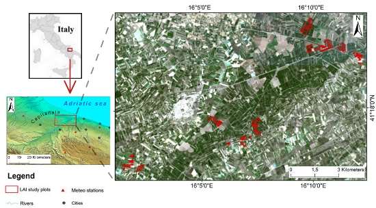
The study area is located in the Apulia region (Figure 1) in the southeastern part of the Italian peninsula, where over 70% of the total area is occupied by agriculture and vineyards cover about 26% of the crop area [40]. The regional topography is mainly flat or slightly sloping, with the exception of the Gargano area, situated in the northwest of the region. The climate of the study area is classified as Mediterranean semi-arid, characterized by moderately cold and rainy winters and dry summer seasons. Mean annual precipitation is about 550 mm, concentrated in the fall and winter; long-term mean air temperature is 15.4 °C, while the minimum and maximum yearly temperatures are 3.5 and 29.5 °C, respectively. The climate, rainfall in particular, exhibits a marked inter-annual variability that makes water availability a permanent threat to the economic development and ecosystem conservation of the region [41]. The soil is typical of the Capitanata region, with a well-differentiated profile, characterized by Quaternary marine sediments of illitic/smectitic composition that originate clay soils with vertic features (cambisols, entisols, vertisols) [42]. Due to its geo-climatic conditions, the region suffers from overall water exploitation, which exposes the water supply system to severe water scarcity events.

Figure 1. Study area location with overview of LAI plot measurements. Natural color composition of Landsat 8 image acquired on 26 August 2014.

Figure 1. Study area location with overview of LAI plot measurements. Natural color composition of Landsat 8 image acquired on 26 August 2014.

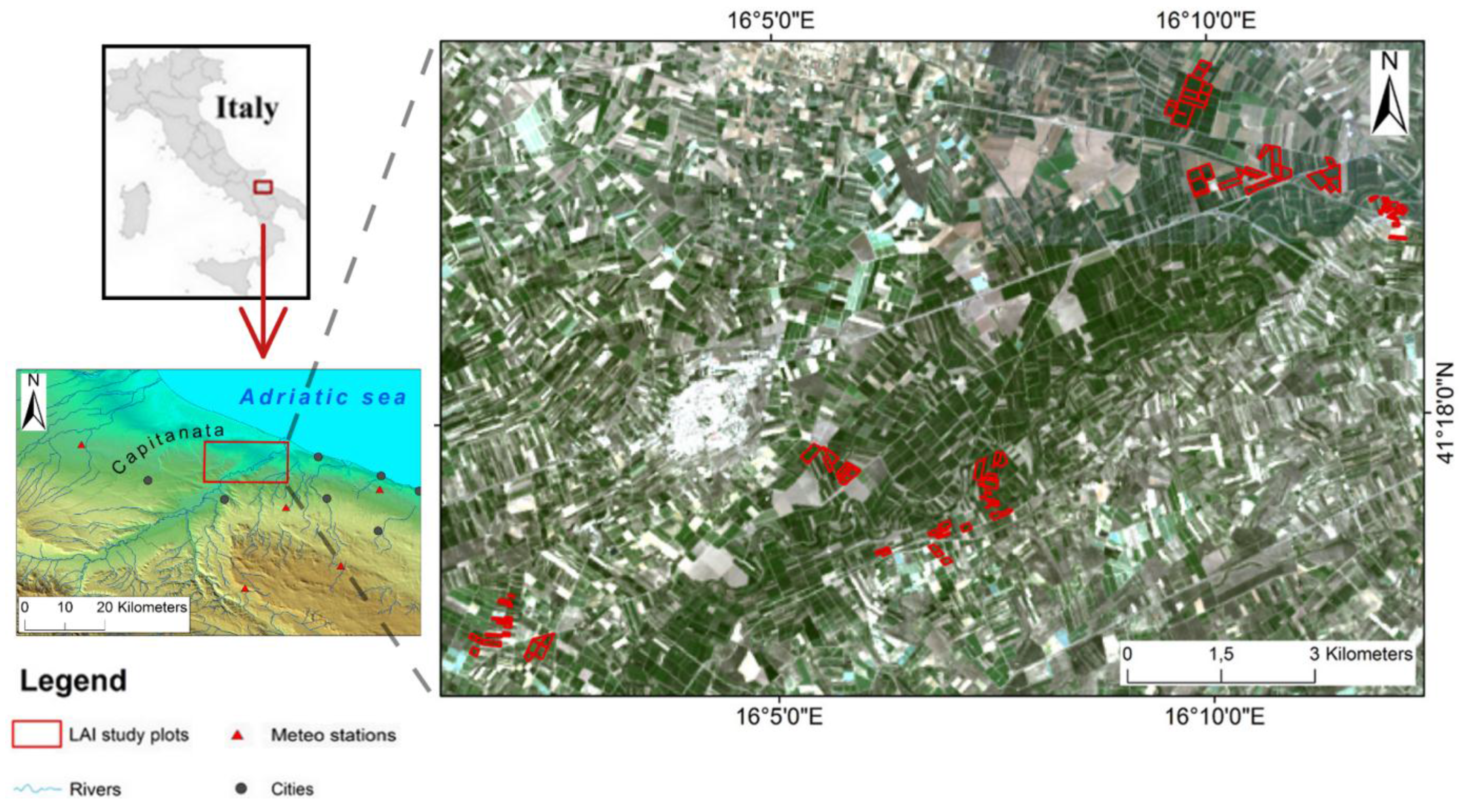
The investigations have been carried within the Land Reclamation and Irrigation Consortium Capitanata, one of the largest agricultural irrigation districts of Southern Italy (Figure 1). This region mainly contains vineyards and orchards over flat terrain. In particular, field data have been collected in a 13 ha multiplot vineyard (41°17ʹ29ʹʹ North latitude, 16°07ʹ22ʹʹ West longitude) trained on a “tendone” system, with commercial table grapes (cultivars Italia, Victoria, and RedGlobe), uncovered and drip irrigated (Figure 2). The row and vine spacing in the vineyard was generally 2.3 × 2.3 m, about 2 m high with a plant density of 1890 plants·ha⁻¹. Agronomic management generally maintains the vegetation under non-water stress conditions and soil surface free of weeds and cover crop.

Figure 2. (a) Overall view of the vineyard study field displayed on a RapidEye image acquired on 2 August 2014 (infrared false color composition 532). Yellow borders show the experimental plots. (b) Canopy growth of the vineyard inter-row acquired on 24 July 2014.

Figure 2. (a) Overall view of the vineyard study field displayed on a RapidEye image acquired on 2 August 2014 (infrared false color composition 532). Yellow borders show the experimental plots. (b) Canopy growth of the vineyard inter-row acquired on 24 July 2014.

2.2. Dataset

The dataset includes Landsat 8 and RapidEye optical images (in the visible and near infrared ranges), agrometeorological data, and in situ Leaf Area Index (LAI) measurements.

2.2.1. Satellite Images

Earth Observation images used to estimate crop coefficients were collected from the sensor OLI (Operational Land Imager), onboard the Landsat 8 Mission (formerly the Landsat Data Continuity Mission, LDCM). The data are available for download free of charge from the U.S. Geological Survey-USGS Earth Explorer data repository.

In addition, several RapidEye high-resolution images at 6.5 m Ground Sample Distance at nadir (generally resampled to 5-m pixel size), were also acquired. The study field concerns two frames of Landsat 8 images (Path 188, Row 31), radiometrically calibrated and orthorectified using ground control points, and a set of high-resolution RapidEye images, radiometrically calibrated. Table 1 summarizes the cloud-free satellite data used and processed over the study area. The temporal frequency of the entire data set acquired allows us to monitor the vegetation development throughout the growing seasons.

Table 1. Overview of the imagery dataset used in the study area.

Satellite Data	GSD* (m)	Processing Level	Revisit Time	N. of Images	Acquisition Dates
Landsat 8 OLI	30	1T	16 day	14	from 19/05/2013 to 26/08/2014
RapidEye MSI	6.5	1B	1 day	10	from 10/06/2014 to 29/09/2014

Note: *Ground sample distance.

Table 1. Overview of the imagery dataset used in the study area.

Satellite Data	GSD* (m)	Processing Level	Revisit Time	N. of Images	Acquisition Dates
Landsat 8 OLI	30	1T	16 day	14	from 19/05/2013 to 26/08/2014
RapidEye MSI	6.5	1B	1 day	10	from 10/06/2014 to 29/09/2014

Note: *Ground sample distance.

2.2.2. Agrometeorological Data and Field Data

Agrometeorological data were acquired from five stations managed by Assocodipuglia, the agrometeorological service of the Apulia Region. Daily data of precipitation, evapotranspiration, atmospheric pressure, global radiation, air temperature, humidity, and wind speed were acquired for both years. Daily air temperature was used to calculate the GDD index from 1 April to 31 October, computed as the difference between the daily mean temperature and the base temperature (10 °C) [43]. In addition, other ancillary and administrative data were used to improve elaborations.

2.2.3. In Situ LAI

In situ LAI measurements (m²·m⁻²) were collected on 23 and 24 July 2014 for 38 sample plots. Field non-destructive measurements of LAI and leaf mean tilt angle were made with LICOR LAI-2000 Plant Canopy Analyzer [44], which works by comparing the intensity of diffuse incident illumination measured at the bottom of the canopy with that arriving at the top. In order to reduce the effect of multiple scattering on LAI-2000 measurements, the instrument was only operated near dusk and dawn (6:30–9:30 am; 6:30–8:30 pm) under diffuse radiation condition, using one sensor for both above and below stand measurements. In order to prevent interference caused by the operator’s presence and the illumination condition, the sensor field of view was limited with a 180° view-cap. Measurements were azimuthally oriented opposite to the sun azimuth angle. LAI measurements were taken with the instrument held a few centimeters above the soil, generally within three days of image data acquisition.

A measurement of ambient light was made with the sensor extended upward and over the top of the canopy at arm’s length. Eight below-canopy readings were then made. This pattern has been repeated three times per spot, and the resulting 24 samples comprise one full set of measurements. Finally, each center of the LAI-2000 transects was geolocated by using GPS (Global Position System) measurements. This measurement protocol allowed us to determine statistically meaningful LAI values, characterized by a low ratio between the standard error of the LAI (SEL) and LAI (SEL/LAI ranged between ≈0.03 and ≈0.07); thus, the actual LAI should be within 10% of the LAI sample mean (Figure 3).

2.3. Methods

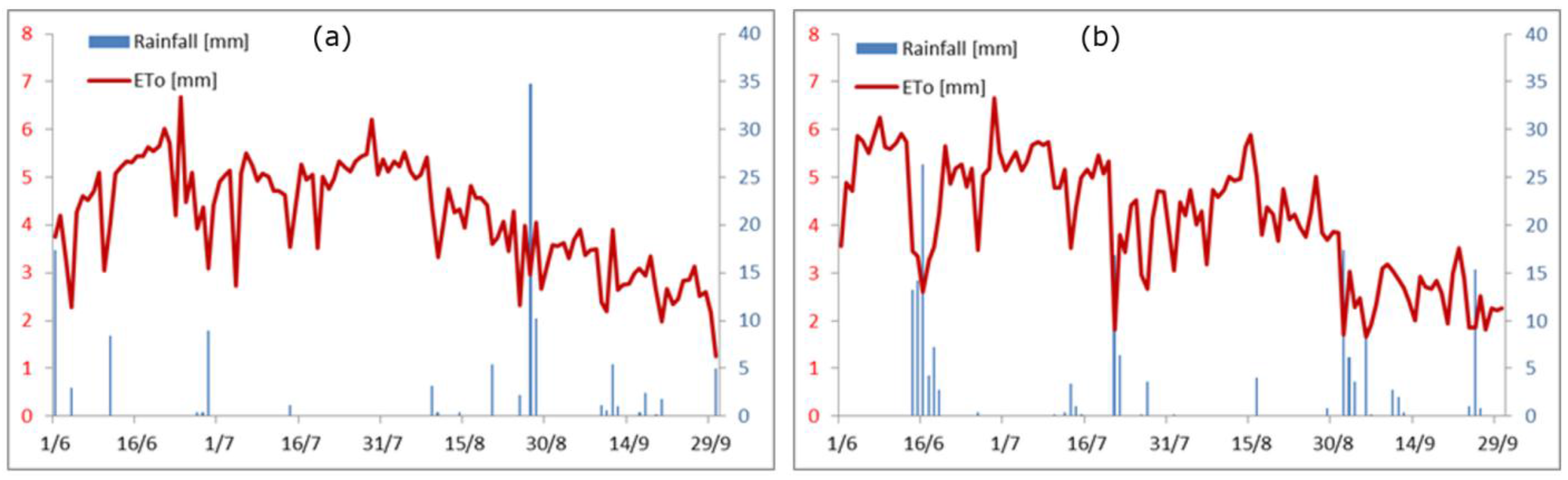
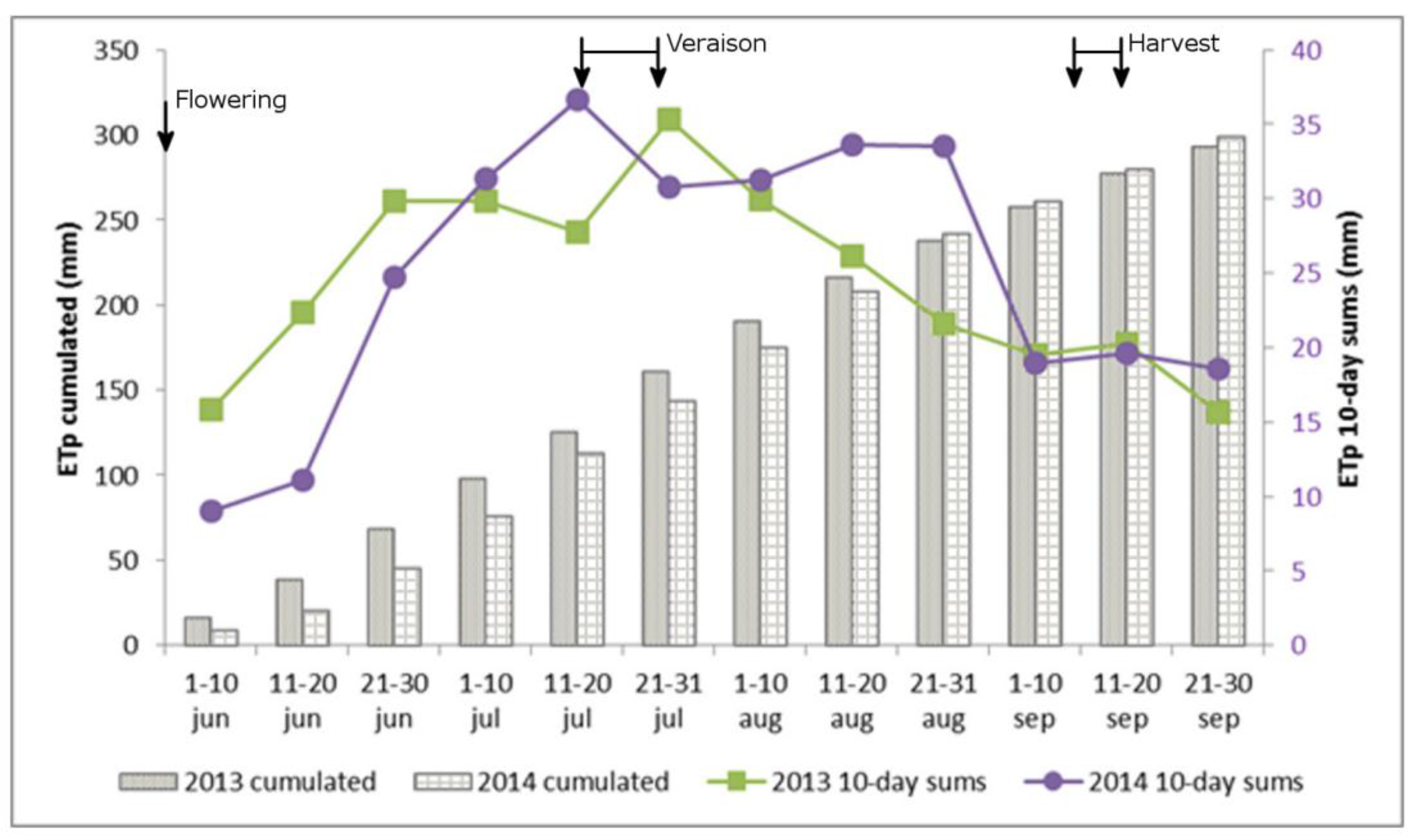
The application of the procedure is achieved by the integration of EO techniques and meteorological data of the study area. The conceptualization has been developed by D’Urso [45] and implemented into the SIMODIS model (SImulation and Management of On-Demand Irrigation System). The estimation of crop evapotranspiration under standard conditions (ET_p—mm/d)—disease-free, adequate fertilization, and soil water availability—has been carried out using the FAO’s Penman–Monteith method, which requires standard meteorological data such as solar radiation (S), air temperature (T_a), air humidity (RH), wind speed (U), and biophysical parameters that are crop-specific, such as albedo (r), LAI, and crop height (h_c) [20]. The value of ET_p is a function of the crop parameters and meteorological data, and the procedure, known as the one-step approach, is computed as:

$$E{T}_p=f\{r,LAI,hc|Ta,RH,S,U\}$$

(1)

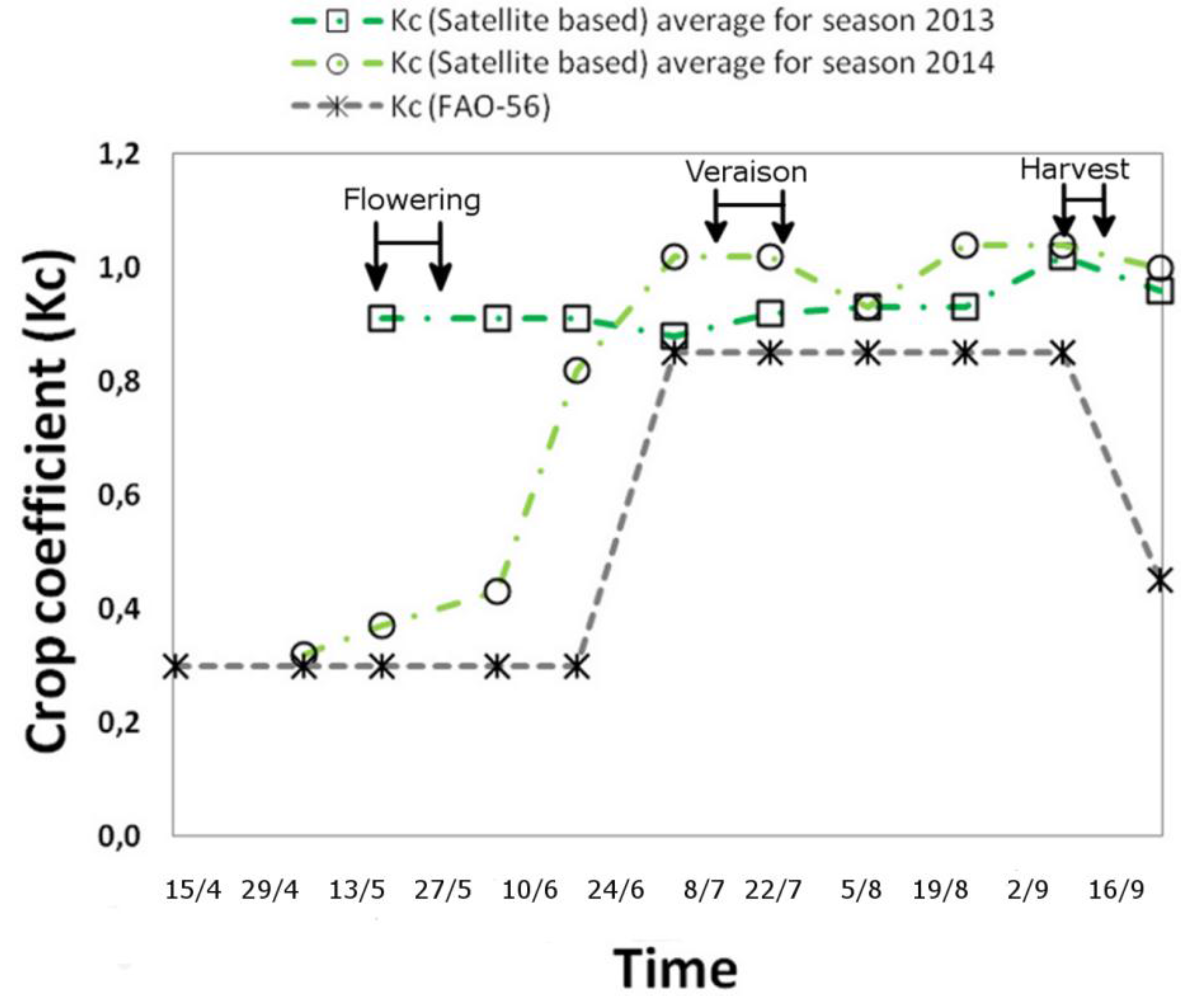
Since crop parameters (mainly r and LAI) are very difficult to obtain in the open field without specific instruments, ET_p is calculated in the routine irrigation management by multiplying ET₀ by K_c, starting from an ET₀ assuming an ideal crop with standard parameters (h_c = 0.12 m, r = 0.23, LAI = 2.88) and a K_c extracted from the FAO-56 table, following a single K_c approach [20].

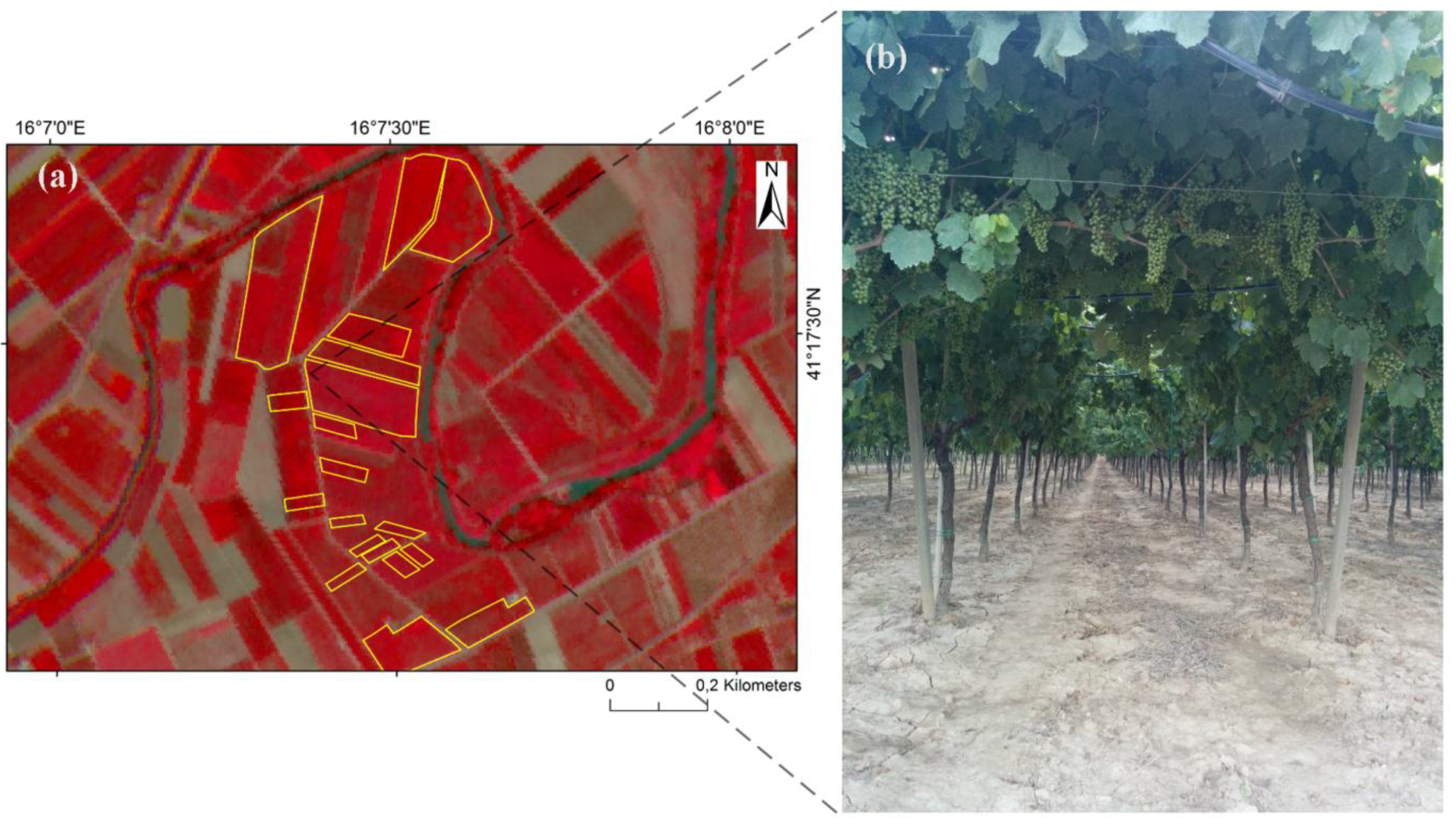
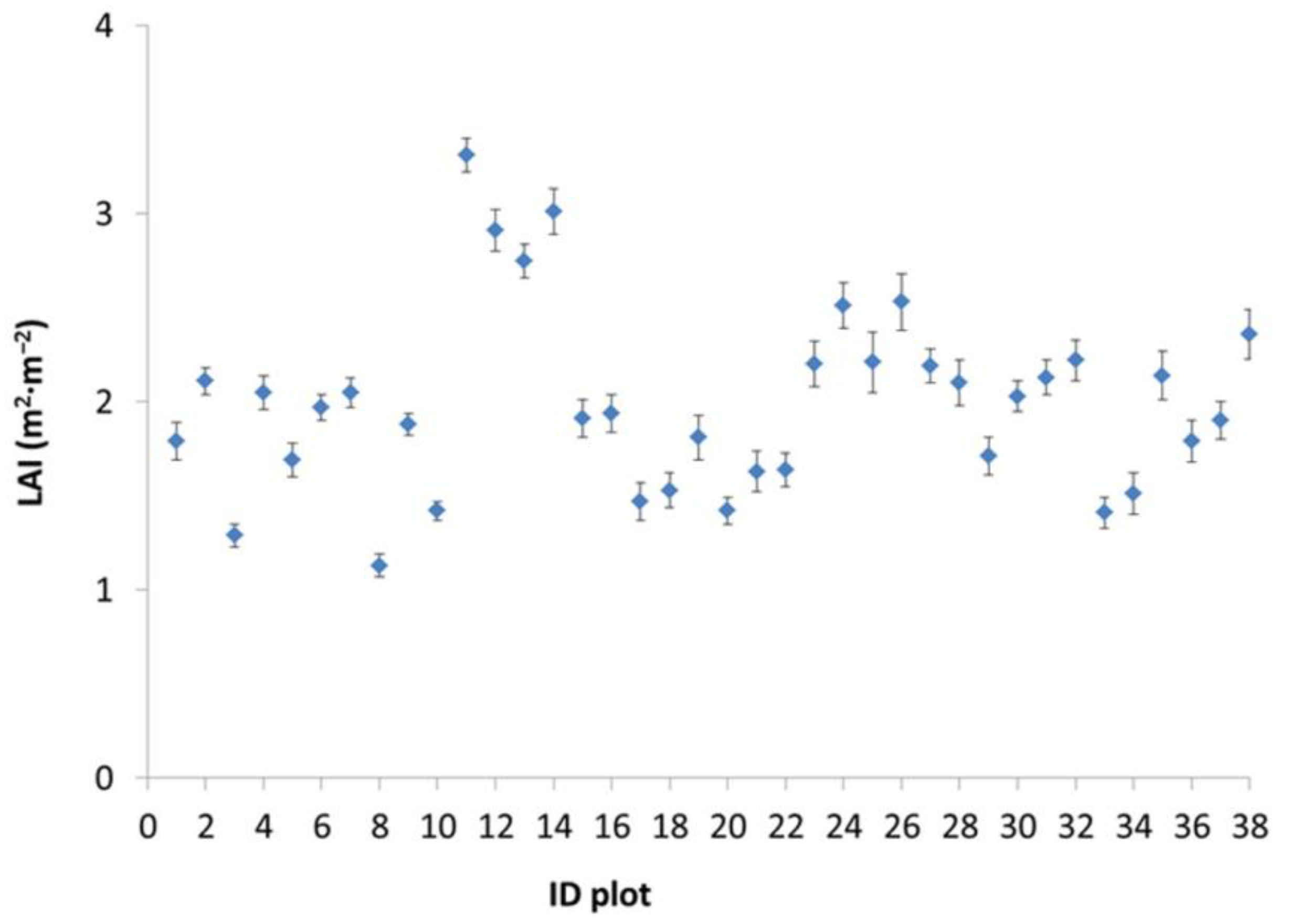
Figure 3. Field estimates of LAI collected on 23–24 July 2014 with a LICOR LAI-2000 Plant Canopy Analyzer. The filled circles show the average LAI with the standard error.

Figure 3. Field estimates of LAI collected on 23–24 July 2014 with a LICOR LAI-2000 Plant Canopy Analyzer. The filled circles show the average LAI with the standard error.

It should be noted that ET_p calculated in this way represents the maximum value, (i.e., minimum canopy resistance), so the resulting K_c values, if compared with values reported in the literature, should be used with caution. The comparison between the results of the proposed methodology and field measurements—including fluxes of latent heat by means of micrometeorological instrumentations—requires fully controlled conditions (especially for irrigation), which were not available at the current study site. However, we assume that the model can be applied to the studied canopy, having been validated in the course of field experiments on different fully irrigated crops [29,39]. Actual evapotranspiration from a well-watered crop will generally approach ET_p during the active growing stage, but it falls below it toward the end of the growing season as the plants begin to dry out. Diversely from our ET₀ estimates, actual evapotranspiration depends on the conditions of soil water availability, and is only possible to compute through complex measurements in the open field or by filling out a detailed hydrological balance, taking into account all the parameters for the simulation of water transport/flow in the Soil, Plant Atmosphere system, using numerical schematization. In this case, the value of ET_p determined with the approach proposed here is used as an upper limiting condition [46]. This kind of analysis has been carried out for some perennial tree crops in Sicily [47], where soil water and surface energy balances with visible, near, and thermal infrared data have been carried out. These previous studies support the assumption of validity, provided that the canopy parameters, i.e., LAI, are adequately described. Finally, crop water requirements can be accounted for in a simple way by subtracting the net precipitation (P_n) from ET_p.

In order to describe the amount of intercepted water from the plant surface, P_n is calculated as a function of the actual precipitation (P), LAI, and fractional cover. The semi-empirical model of interception [48] is described by the following relationship:

$$P_n=P-aLAI\left(1-\frac{1}{1+\frac{f\text{cover}\cdot P}{aLAI}}\right)$$

(2)

where P (cm·d⁻¹) and a (cm·d⁻¹) are empirical parameters representing the crop saturation per unit foliage area (~0.28 for most crops), and fcover is the fractional vegetation cover derived from LAI using a polynomial empirical expression where coefficients are determined from field measurements and are valid for a wide range of crops (LAI ≤ 5 m²·m⁻²).

K_c values are extremely variable, even within the same type of crop, depending on many factors, i.e., date and seeding density, intake of nutrients, nature of the soil, and agronomic practices. K_c is basically the ratio of the ET_p to the ET₀, and can be computed as follows [45,49]:

$$K_c=\frac{E{T}_p(r^{*},LA{I}^{*},h{c}^{*},Ta,RH,U,K^{\downarrow })}{E{T}_0(r,LAI,hc,Ta,RH,U,K^{\downarrow })}$$

(3)

where r^*, LAI^* and h_c^* represent the parameters of the crop vegetation present at the time of the satellite overpass, which can be related to satellite observations, while K^↓ represent the global incoming short-wave radiation flux density. The value of K_c depends both on the crop parameters (except albedo, which is also influenced by the degree of humidity of the soil), which can be considered relatively stable for a period of 1–2 weeks, and the weather conditions of the study area, which instead vary in time. A sensitivity analysis of the value of K_c with respect to these parameters showed that the value of K_c is more closely related to vegetation parameters r^* and LAI^*, and that the sensitivity of the change in the crop height is higher in autumn than in summer [45]. This is due to the fact that, at the daily scale, the aerodynamic component of evapotranspiration is of much less importance than the radiative. A flow-chart of the processing chain of this procedure can be found in Vuolo et al. [39]. The validation has been carried out over different crops (including vineyards), thereby fulfilling the “standard conditions” for ET_p by means of eddy-covariance independent measurements [29,39]. Since LAI represents the main parameter, it can be taken as the reference variable for the calibration of this method to local conditions, as described later.

Recent studies conducted in semi-arid areas confirm this trend [50]; in fact, a percentage change of 50% in h_c^* corresponds to a variation of 5% of K_c. Therefore, a constant value of h_c = 0.4 m has been set in this study, valid for the climatic conditions of the Mediterranean area, reducing the calculation to the estimation of r and LAI.

Data Processing for Deriving EO-Based Crop Development Maps

A total of 14 Landsat 8 images and 10 RapidEye images were used for both growing seasons. The pre-processing phase of satellite images was achieved in two steps. Firstly, Landsat 8 scenes were orthorectified by using additional Ground Control Points and a Digital Elevation Model, while RapidEye scenes were orthorectified using only the image’s rational functions. Secondly, the images have been atmospherically corrected using the ATCOR-2 software suite in ERDAS imagine, which incorporates the MODerate resolution atmospheric TRANsmission (MODTRAN version 4) model and uses look-up tables with pre-calculated model simulations for different satellite sensor types and a range of atmospheric conditions [51,52]. Furthermore, supervised classification of Landsat 8 images was performed to identify at each acquisition the plots of agricultural land cover with vegetation and areas with bare soil and/or urban areas.

In order to implement the FAO-56 model, for each satellite image a set of maps of K_c were derived on the basis of LAI and r maps. The surface albedo, needed to derive the net radiant flux, is an approximation of the hemispherical and spectrally integrated surface albedo, and was extracted as part of the value-added products available in ATCOR-2 after the atmospheric correction [53]. 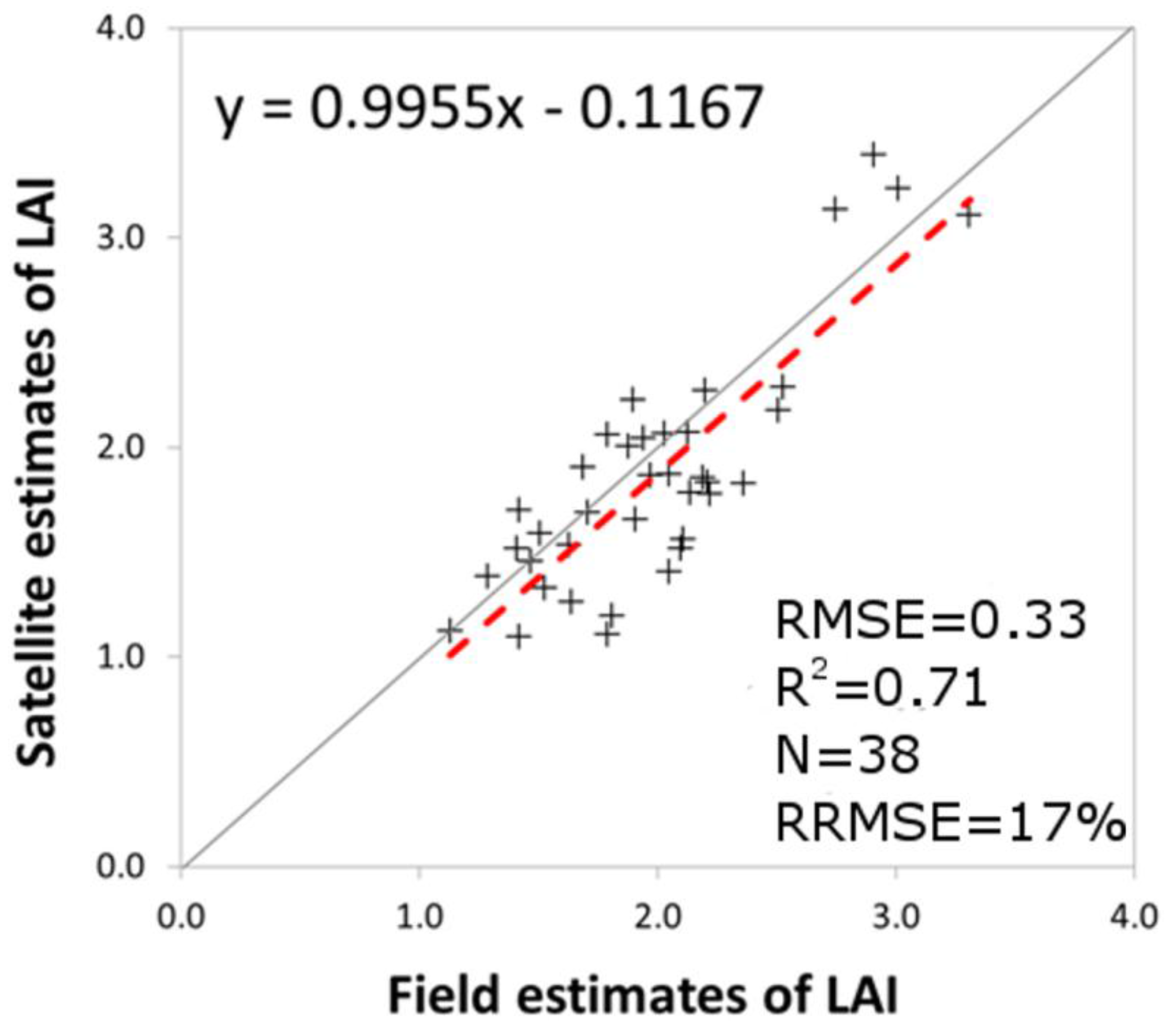LAI is a biophysical surface parameter defined as the total one-sided area of photosynthetic tissue per unit of ground area [54]. The estimate of the LAI was performed based on the simplified Clevers’ Leaf Area Index by Reflectance model, CLAIR [55], based on the Weighted Difference Vegetation Index (WDVI). The WDVI is a radiometric index calculated, for each pixel of the image, from the values of reflectance r_sRED and r_sNIR, respectively, in the bands of red (0.63–0.69 μm) and the near infrared (0.76–0.90 μm). The ratio of near-infrared and red soil reflectance is also known in the literature as the “soil line slope,” usually between 0.9 and 1.3. The effect of weighting the red band with the slope of the soil line is the maximization of the vegetation signal in the near-infrared band and the minimization of the effect of soil brightness. The LAI is related with WDVI of the observed vegetation, through the following expression, deduced from a simplified analysis of the radiative behavior of different types of crops [50,55,56]:

$$LAI=-\frac{1}{{\alpha }^{*}}\ln (1-\frac{WDVI}{WDV{I}_{\infty }})$$

(4)

where α* is an extinction coefficient (increase of WDVI for an unitary increase of LAI—an empirical shape parameter, mainly depending on canopy architecture and computed from field measurement and considered to be 0.39 in this study, corresponding to the minimum error between the observed and estimated LAI), and WDVI∞ is the asymptotical value of WDVI for LAI→∞, and is calculated at each acquisition at the target “vegetation cover (not woody) very dense and uniform” or maximum vegetation (agricultural) cover (usually between 0.55 and 0.75).

In situ LAI measurements have been used to produce LAI maps from Landsat 8 and RapidEye images by applying the semi-empirical CLAIR model based on an inverse relationship between the WDVI and LAI [55,57].

The CLAIR model needs to be calibrated by estimating the extinction coefficient α*. Equation (4) must be inverted, fixing the LAI, WDVI, and WDVI∞ values. WDVI∞ was calculated (r_sNIR/r_sRED = 1.35, WDVI∞ = 0.55) so as to create a correspondence of pixels with maximum vegetation cover. The resulted α* values were in the range of 0.34–0.70. The final value of α* = 0.39 corresponds to the minimum error between observed and estimated LAI, leading to an average error of 25% in the estimation of the LAI. To test the model prediction accuracies, we used the root-mean-square error (RMSE) and the coefficient of determination (R²) between measured and predicted LAI. According to the FAO-56 model, the ET₀ computed from the agrometeorological variables using the Penman–Monteith equation is used to calculate the value of K_c (according to the analytical method), where K_c is the ratio between ET_p and ET₀ [20]. K_c incorporates and synthesizes all the effects on the evapotranspiration related to morpho-physiological characteristics of the different crops—phenological stage, degree of soil cover, soil and climate conditions—that make them different from the reference crop.

The mean value of the ratio between ET_p and ET₀ over a period of about seven days around the date of satellite’s passage is applied twice, once with standard values of LAI, r, and crop height for a reference surface, and once by using the LAI, r, and crop height (this latter is fixed for tree crops) from satellite images. To speed up this processing in a GIS environment, we derive a polynomial expression of degree 4, whose coefficients are derived by calculating the K_c intervals of LAI and albedo targets (i.e., LAI in range 0–5 and step 0.2; albedo in range 0.05 to 0.5 and step 0.01). The coefficients mostly depend on meteorological data, and they are dimensionless as LAI and K_c. This procedure is not strictly needed, since we could directly use the FAO-56 method on a daily basis, but it has the advantage of showing the direct link between K_c, LAI, and albedo. Once we derive albedo and LAI from the satellite images and calculate the coefficients for a given time interval, in a GIS environment we derive the K_c map on a pixel-by-pixel basis. One important advantage of deriving canopy parameters or crop coefficients from spectral measurements is that their values do not depend on other variables such as planting date and density, but on the effective cover.

3. Results and Discussion

3.1. Weather Conditions, Reference ET, and Phenology

Rainfall and temperature in 2013 and 2014 were slightly different but in accordance with climatological averages for the study area (Figure 4). The year 2013 has been characterized by a rainy winter and spring and a dry summer, with anomalously high precipitation in August and in the autumn, while 2014 experienced a rainy spring: long-term average precipitation from April to June was 210 mm, about 35% of the annual amount. This situation affected the crop water requirements during the growing season. Annual rainfall and mean temperature were 629.2 mm and 16.2 °C for 2013, and 607.4 mm and 16.7 °C for 2014, respectively. Total rainfall from 1 June to 30 September was 114.4 mm (18% of the annual amount) in 2013 and 103 mm (27% of the annual amount) in 2014, respectively.

Seasonal variations of ET₀ are shown in Figure 5 for 2013 and 2014, respectively. The total amounts of ET₀ in the growing season (1 June to 30 September) were similar in both years: 511 mm in 2013 and 501.6 mm in 2014. The average daily ET₀ was 4.2 mmd⁻¹ and 4.1 mmd⁻¹ in the first and second year, respectively. In the 2013 growing season the lowest daily ET₀ was 1.3 mmd⁻¹ (30 September) and the highest was 6.7 mmd⁻¹ (24 June). In the 2014growing season, ET₀ values ranged from 1.7 mmd⁻¹ (1 September) to 6.7 mmd⁻¹ (29 June). The transpiration values reported in this study are consistent with those reported by Suvocӑrev et al. [22] (4.3–4.4 mmd⁻¹) and Teixeira et al. [2] (3.9–4.4 mmd⁻¹) for table grapes trained on an overhead trellis system, although they cannot be directly compared because they were measured at the ground.

Figure 4. Seasonal trends of temperature and rainfall at an agrometeorological station in Andria for the years 2013 (a) and 2014 (b).

Figure 4. Seasonal trends of temperature and rainfall at an agrometeorological station in Andria for the years 2013 (a) and 2014 (b).

Figure 5. Seasonal trends of ET₀ and rainfall events during the growing season for the years 2013 (a) and 2014 (b).

Figure 5. Seasonal trends of ET₀ and rainfall events during the growing season for the years 2013 (a) and 2014 (b).

In addition, the GDD index was calculated using the data from a weather station located near the sample plots. The length of four key phenological stages was also identified based on mean dates registered in the study area. The GDD index from 1 April to 31 October is similar for both seasons and ranged from 2108 GDD in 2013 to 2128 GDD in 2014 (Table 2), thus the study area was classified as Region IV (hot) [58]. Nevertheless, the GDD accumulation up to flowering in the 2014 growing season was markedly lower than in 2013.

Table 2. Phenological stages and cumulative GDD during the 2013 and 2014 growing seasons.

Phenology *	Time	GDD 2013	GDD 2014
Bud break	1–6 April	0	0
Flowering	20–30 May	341	279
Veraison	16–24 July	981	1040
Harvest	10–15 Sept.	1747	1766
–	31 October	2018	2128

Note: * Observed mean dates of key phenological stages were obtained from the research unit Consiglio per la Ricerca in Agricoltura e l’Analisi dell’Economia Agraria UTV, Turi (Tarricone L., personal communication).

Table 2. Phenological stages and cumulative GDD during the 2013 and 2014 growing seasons.

Phenology *	Time	GDD 2013	GDD 2014
Bud break	1–6 April	0	0
Flowering	20–30 May	341	279
Veraison	16–24 July	981	1040
Harvest	10–15 Sept.	1747	1766
–	31 October	2018	2128

Note: * Observed mean dates of key phenological stages were obtained from the research unit Consiglio per la Ricerca in Agricoltura e l’Analisi dell’Economia Agraria UTV, Turi (Tarricone L., personal communication).

The accumulation of degree-days has important implications for the length of the growth stages and water availability [59]. In fact, it has been demonstrated that canopy development is highly correlated with GDD [12,60] and consequently the canopy cover and shaded area control the seasonal values of the K_c [12]. Overall, these studies suggested that the observed K_c values should be linked to the cumulative GDD of specific agro-climatic locations in order to minimize the effects of year-to-year weather variations. Clearly, the seasonal development and length of growing stages on other study areas can be very different compared with those considered by the FAO-56 paper.

Up to now, a number of studies pointed out that changes in climate led to significant impacts on the phenology time series, for example shifts in phenological timing of bud-burst to harvest [25,61,62]. These results further support the need for setting K_c values for the new climate change projections, as well as agronomic practices aimed at the enhancement of soil water availability (i.e., mulching, netting, and biochar) [11,22,63].

3.2. Temporal Evolution of LAI and Kc

Consequently, the measurements made in the field were compared with the data elaborated from high-resolution satellite images (RapidEye). The data are an average of the pixels belonging to the same polygon of land cover. The scatterplot between field LAI measured and satellite LAI estimates are shown in Figure 6. The RMSE and R² between measured and predicted LAI are 0.33 and 0.71, respectively.

Figure 6. Scatter plots (n = 38) of field LAI estimates (23 to 24 July 2014) and satellite estimates of LAI (RapidEye image, 2 August 2014). RMSE: root mean square error. R² = coefficient of determination. RRMSE: relative root mean square error. The broken red line shows the ordinary least squares linear regression fits. In black is the 1-to-1 line.

Figure 6. Scatter plots (n = 38) of field LAI estimates (23 to 24 July 2014) and satellite estimates of LAI (RapidEye image, 2 August 2014). RMSE: root mean square error. R² = coefficient of determination. RRMSE: relative root mean square error. The broken red line shows the ordinary least squares linear regression fits. In black is the 1-to-1 line.

Seasonal K_c values were obtained by dividing ET_p with the reference evapotranspiration calculated as previously described. The time evolution of measured K_c for the growing seasons 2013 and 2014 are reported in Table 3 and Table 4, respectively. During the 2013 growing season the K_c value moves from a minimum of 0.43 to a maximum of 1.23 on the date of harvest, while in 2014 the K_c moves from a minimum of 0.14 to a maximum of 1.42. The K_c mean values were higher in May and June in 2013, and from July to the beginning of September in 2014. Unfortunately, there is no data available for September 2014, since the month was very rainy and the cloud coverage of satellite images did not allow us to elaborate any data. Initial K_c in the 2013 growing season was high and constant around 0.90, with a maximum value of 1.02 close to the harvest, in September. Overall, the standard deviation values of the 2014 data are lower than for the 2013 data, denoting good stability and fairly tight dispersion in the dataset.

Table 3. Statistical parameters for K_c values derived from Landsat 8 satellite images from the year 2013 (n = 110 plots).

Kc	19 May 2013	20 June 2013	06 July 2013	22 July 2013	07 August 2013	23 August 2013	08 Sept 2013	24 Sept 2013
maximum	1.14	1.14	1.14	1.19	1.19	1.18	1.23	1.19
average	0.91	0.91	0.88	0.92	0.93	0.93	1.02	0.96
minimum	0.58	0.58	0.43	0.46	0.48	0.49	0.58	0.56
Standard deviation	0.13	0.13	0.15	0.15	0.14	0.14	0.13	0.13

Table 3. Statistical parameters for K_c values derived from Landsat 8 satellite images from the year 2013 (n = 110 plots).

Kc	19 May 2013	20 June 2013	06 July 2013	22 July 2013	07 August 2013	23 August 2013	08 Sept 2013	24 Sept 2013
maximum	1.14	1.14	1.14	1.19	1.19	1.18	1.23	1.19
average	0.91	0.91	0.88	0.92	0.93	0.93	1.02	0.96
minimum	0.58	0.58	0.43	0.46	0.48	0.49	0.58	0.56
Standard deviation	0.13	0.13	0.15	0.15	0.14	0.14	0.13	0.13

Table 4. Statistical parameters for K_c values derived from Landsat 8 satellite images from the year 2014 (n = 110 plots).

Kc	06 May 2014	07 June 2014	23 June 2014	09 July 2014	10 August 2014	26 August 2014
maximum	0.63	0.75	1.07	1.42	1.10	1.30
average	0.32	0.43	0.82	1.02	0.93	1.04
minimum	0.14	0.17	0.53	0.68	0.56	0.63
Standard deviation	0.08	0.10	0.11	0.16	0.10	0.12

Table 4. Statistical parameters for K_c values derived from Landsat 8 satellite images from the year 2014 (n = 110 plots).

Kc	06 May 2014	07 June 2014	23 June 2014	09 July 2014	10 August 2014	26 August 2014
maximum	0.63	0.75	1.07	1.42	1.10	1.30
average	0.32	0.43	0.82	1.02	0.93	1.04
minimum	0.14	0.17	0.53	0.68	0.56	0.63
Standard deviation	0.08	0.10	0.11	0.16	0.10	0.12

The review of vineyard K_c values for table grapes available in literature is described in Table 5. Initial K_c in 2014 growing season is 0.32–0.43, closer to the value obtained by Netzer et al. [64] in Israel and Lamaddalena and Caliandro [65] in the same region of our study area. Midseason K_c in our study area in the two growing seasons was around 0.8 and 1.02, in line with those values reported by Rana [36] in Apulia, and Williams and Ayars [12] in California. The peaks of 1.23 in 2013 and 1.42 in 2014 are consistent with those of Netzer et al. [64], Villagra et al. [66], and Williams and Ayars [12]. All these authors estimated a K_c value equal to or greater than 1.2 for table grapevine varieties: “Thompson seedless” for Villagra et al. [66] and Williams and Ayars [12], and “Superior Seedless” for Netzer et al. [64].

Figure 7 shows the temporal evolution of K_c of “tendone” vineyards in 2013 and 2014 together with the K_c of grapes derived from the FAO-56 paper. Furthermore, arrows marked on the graph indicate the corresponding dates of phenological stages. Regarding the 2013growing season, it is interesting to note that the “usual” trend of K_c is not present, probably due to the higher vegetative growth and canopy cover stimulated by high temperatures from bud break up to flowering (Table 2) and regular precipitation. As mentioned in the FAO-56 paper [16], accurate estimates for initial K_c should consider the frequency with which the soil surface is wetted during the initial period. Where the soil is frequently wet from irrigation or rain, and consequently there is a greater amount of available water, the evaporation from the soil surface can be considerable and the initial K_c value will be large.

Figure 7. Comparison of Kc (average) estimated from remote sensing data (Landsat 8) and K_c from the FAO-56 table.

Figure 7. Comparison of Kc (average) estimated from remote sensing data (Landsat 8) and K_c from the FAO-56 table.

On the contrary, in the 2014 growing season the trend of estimated K_c value is similar to the K_c FAO trend, with a lower value at the beginning of the season, probably due to low temperatures up to flowering (Table 2), a peak from the first 10 days of July, a slight decrease in the first 10 days of August, and a plateau in the middle of the season. This observation may support the hypothesis that the vegetation growth and K_c trend, after a slow development, was stimulated by GDD accumulation that at veraison surmount the values of the 2013 growing season.

It is interesting to note that the FAO-56 K_c value underestimates the local water need of “tendone” vineyards at all phenological stages. These results are consistent with those of Villagra et al. [66], who reported a K_c value higher than suggested by the FAO-56 paper for Thompson Seedless table grapes in Chile, in growing season 2008–2009 by using the Eddy covariance method. On the contrary, Er-Raki et al. [28] reported K_c values lower than those presented in the FAO-56 paper for Perlette and Superior table grapes in Northwest Mexico (especially for the mid-season) by using ground-based, remotely-sensed data.

However, in the latter case the authors explained their results by the fact that a “Y” open-gable trellis system creates large areas of unshaded bare soil where significant heat fluxes were lost and were not available for transpiration. A possible explanation for these results may be the lack of adequate consideration of vegetation cover, since FAO-56 K_c values were computed for table grapes trained on a trellis system. Furthermore, this critique was confirmed by Williams and Ayars [12], who suggested that K_c and water use are linear functions of the shaded area measured beneath the canopy.

A significant analysis and discussion of this subject was presented by Allen and Pereira [67], who proposed a general procedure for estimating K_c where ground cover and height vary between orchards. In this study the K_c values for the initial, mid-season, and end-season periods were set to 0.30, 1.10, and 0.85 for a ground cover of 70%, 0.30, 0.95, and 0.75 for a ground cover of 50%, and 0.30, 0.60, and 0.5 for a ground cover of 25%.

Overall, these findings suggest that K_c in different crop management systems (e.g., trellising and canopy structure) and agro-climatic locations can vary widely and should be accurately estimated for better irrigation scheduling instead of using the fixed values reported in the literature [12].

Table 5. K_c values of table grapes reported in bibliography.

Kc			Trellis System	Cultivar	Season	Country	References
Initial	Middle	End
–	~1	–	Tendone	Italia	1997	Italy	Rana et al. [36]
0.2	0.9–1.3	–	Head training system	Thompson seedless	1998–1999	California	Williams and Ayars [12]
0.48	0.68	0.68	Tendone	–	–	Italy	Lamaddalena and Caliandro [65]
0.4	1–1.2	1.3	Open-gable	Superior seedless	2004–2005	Israel	Netzer et al. [64]
0.22	0.45	0.3	Open-gable	Perlette & Superior seedless	2005–2006	Mexico	Er-Raki et al. [28]
–	0.79	0.98	Open-gable*	Red Globe	2007–2008	Spain	Moratiel and Martinez-Cob [68]
0.54	0.65	0.9	Overhead trellis system*	Crimson seedless	2008–2009	Spain	Suvocarev et al. [22]
0.47	0.60	–	Overhead trellis system*	Autumn Royal	2009	Spain
0.2–0.4	~0.9–1.2	1.2	Overhead trellis system	Thompson seedless	2008–2010	Chile	Villagra et al. [66]

Note: * Vineyard covered with a net made of a thread warp of high-density polyethylene.

Table 5. K_c values of table grapes reported in bibliography.

Kc			Trellis System	Cultivar	Season	Country	References
Initial	Middle	End
–	~1	–	Tendone	Italia	1997	Italy	Rana et al. [36]
0.2	0.9–1.3	–	Head training system	Thompson seedless	1998–1999	California	Williams and Ayars [12]
0.48	0.68	0.68	Tendone	–	–	Italy	Lamaddalena and Caliandro [65]
0.4	1–1.2	1.3	Open-gable	Superior seedless	2004–2005	Israel	Netzer et al. [64]
0.22	0.45	0.3	Open-gable	Perlette & Superior seedless	2005–2006	Mexico	Er-Raki et al. [28]
–	0.79	0.98	Open-gable*	Red Globe	2007–2008	Spain	Moratiel and Martinez-Cob [68]
0.54	0.65	0.9	Overhead trellis system*	Crimson seedless	2008–2009	Spain	Suvocarev et al. [22]
0.47	0.60	–	Overhead trellis system*	Autumn Royal	2009	Spain
0.2–0.4	~0.9–1.2	1.2	Overhead trellis system	Thompson seedless	2008–2010	Chile	Villagra et al. [66]

Note: * Vineyard covered with a net made of a thread warp of high-density polyethylene.

3.3. Temporal Evolution of Evapotranspiration

Figure 8 provides an overview of the cumulated ET_p and 10-day sums trend line during the period between 1 June and 30 September for both growing seasons. In addition, arrows marked on the graph indicate the dates of the main phenological stages. The average ET_p value ranged from 294 mm in 2013 to 299 mm in 2014. These results can be compared with those obtained by Texeira et al. [2], who reported a mean value ET_p of 372 mm, although, as highlighted by Netzer et al. [64], the comparison between seasonal ET_p in different regions and different practices can be misleading and might lead to misinterpretations of the results and incorrect inferences.

Figure 8 is quite revealing and interesting in several ways, showing differences especially at mid-season. Firstly, the cumulative values for the year 2013 are generally higher than those in year 2014 until the first 10 days of August, while the values have similar trends up to the end of September. As stated previously when referring to the K_c trend lines, these differences can be explained by several factors. First, we need to consider that the 2013 growing season was initially warmer, with enhanced canopy cover and evaporative demand, and consequently improved daily transpiration. Secondly, the 10-day sums of ET_p for both seasons show a trend in line with high atmospheric demand during the summer, but with some peaks and decreasing values linked to rainfall events. For example, for both growing seasons we register the peaks of 10-day sums of ET_p at the days of veraison, but shifted by about 10 days. Furthermore, the peak on the last 20 days of August 2014 might have been influenced by a drought month, while decreasing ET_p values experienced in August 2013 could be attributed to some rain events (about 52 mm in the last 12 days of the month), more abundant and larger than in 2014 (see Figure 4 and Figure 5), that resulted in cloudy and cool conditions. Although mean monthly air temperature was similar for both months (24.4 °C for 2013 and 24.6 °C for 2014), this area is very windy and evapotranspiration trends may also be affected by the wind. Finally, the equal values of ET_p registered toward the end of the season and in correspondence with the harvest can be attributed to reduced evapotranspiration demand and leaf senescence [69]. On the other hand, with regard to the soil water status, it is important to bear in mind that table grape vineyards are constantly irrigated by grape growers to maintain adequate soil water availability to the root-zone.

Figure 8. Cumulative values and trend line evolution of ET_p.

Figure 8. Cumulative values and trend line evolution of ET_p.

Furthermore, crop water requirements calculated during the period June–September as the difference between ET_p and water resulting from precipitation (114.4 mm for 2013 and 164.8 mm for 2014) show an average irrigation requirement of 179.5 mm for 2013 and 134.3 mm for 2014, respectively. The amount of water commonly applied by using drip irrigation in this study area, collected through semi-structured questionnaires engaging grape growers in the 2013season, was approximately 250 mm, close to our ET_p values. Our results indicate that farmers tend to over-irrigate the crop, due to the unavailability of supporting information about climate and canopy development. Interestingly, a recent study in the same study area shows the possibility of reducing crop water requirements by applying seasonal water volumes, equal to 80% of ET_p at the end of irrigation season (about 220–230 mm, in line with our values), with the best balance among grape yield, berry quality, and water use [9]. In addition, visual estimations of time-series in summer 2014 for the LAI, NDVI, K_c, and ET_p are shown in Figure 9. This figure indicates that the ET_p and K_c trend patterns are strictly related with VI at the time of the satellite overpass, but from one date to another are strongly influenced by specific weather conditions and soil moisture. These data show the importance of local climate conditions for water management and irrigation scheduling of the table grapes, and confirm the requirement of site-specific K_c, considering the remarkable seasonality in precipitation during the growing seasons in the study area. Further studies need to be carried out in order to better validate the relation among LAI, K_c, and soil water status.

Figure 9. An example of time-series maps of LAI, NDVI, K_c, and ET_p for the vineyard study field represented in Figure 2.

Figure 9. An example of time-series maps of LAI, NDVI, K_c, and ET_p for the vineyard study field represented in Figure 2.

4. Conclusions

This study evaluates the crop coefficients and evapotranspiration of table grapes trained on a “tendone” system under conditions of unlimited soil water availability, pest and disease-free crop, etc. The method is based on the FAO-56 model by using appropriate values of canopy variables such as the surface albedo and the LAI derived by means of multispectral satellite data, based on existing validated methodologies. The results for the study area in the Apulia region (Italy) indicate that the values of K_c are site- and year-specific and depend on local ET₀ rates, rainfall frequency, cumulative thermal requirements, and effective canopy cover. For instance, during the 2013 growing season the Kc value moves from a minimum of 0.43 to a maximum of 1.23 at harvest, while in 2014 the Kc moves from a minimum of 0.14 to a maximum of 1.42. The obtained results showed good consistency compared with values retrieved from the international literature regarding table grapes in Mediterranean environments, although they should be used with some caution because the calculated ET_p are not the actual values but the maximum values in absence of stress. The resulting crop water requirements are lower than the actual average irrigation volumes applied by farmers, thus suggesting the possibility of improving the water use efficiency of these crops by adopting the proposed methodology. The methodology and results of this research confirm the usefulness of E.O. data in supporting irrigation scheduling and agricultural water management. Furthermore, the approach described in this paper also constitutes the basis for a potential irrigation advisory service using E.O. data as an operational service.