Building a Data Set over 12 Globally Distributed Sites to Support the Development of Agriculture Monitoring Applications with Sentinel-2

Abstract

Developing better agricultural monitoring capabilities based on Earth Observation data is critical for strengthening food production information and market transparency. The Sentinel-2 mission has the optimal capacity for regional to global agriculture monitoring in terms of resolution (10–20 meter), revisit frequency (five days) and coverage (global). In this context, the European Space Agency launched in 2014 the “Sentinel­2 for Agriculture” project, which aims to prepare the exploitation of Sentinel-2 data for agriculture monitoring through the development of open source processing chains for relevant products. The project generated an unprecedented dataset, made of “Sentinel-2 like” time series and in situ data acquired in 2013 over 12 globally distributed sites. Earth Observation time series were mostly built on the SPOT4 (Take 5) data set, which was specifically designed to simulate Sentinel-2. They also included Landsat 8 and RapidEye imagery as complementary data sources. Images were pre-processed to Level 2A and the quality of the resulting time series was assessed. In situ data about cropland, crop type and biophysical variables were shared by site managers, most of them belonging to the “Joint Experiment for Crop Assessment and Monitoring” network. This data set allowed testing and comparing across sites the methodologies that will be at the core of the future “Sentinel­2 for Agriculture” system.

1. Introduction

Achieving sustainable food security for all people was a key priority of the World Food Summit that took place from 13 to 17 November 1996 [1]. This priority was re-affirmed and re-highlighted during the Millennium Summit of the United Nations (UN) in 2000 [2], which defined the eradication of extreme poverty and hunger as one of the eight Millennium Development Goals (MDGs). In 2015, which was the MDGs deadline, broad progress was reported in varying topics, including the poverty reduction target. However, hunger remains an everyday challenge for almost 795 million people worldwide [3].

In June 2011, the need to enhance food security and address commodity price volatility was mentioned for the first time in the declaration following the meeting of the G20 Ministries of Agriculture in Paris [4]. This objective was confirmed in the Final Declaration of the Cannes Summit from November 2011 [5] and re-emphasized in June 2012 in the declaration of the G20 Mexico summit [6]. The international food supply crises as regularly observed since 2008 have further shown how agriculture production and its markets are globally connected and exhibit both a wide geographical variation and high fluctuations over time [7].

It is now widely acknowledged that neither the problem of food insecurity nor the impact of increased market volatility are likely to disappear without policy interventions based on sound scientific evidence [8]. Consequently, it is critical to develop better agricultural monitoring capabilities able to provide timely information about crop status, crop area and yield forecasts [9]. Earth Observation (EO) data can clearly contribute to this objective as a proven source for transparent, timely, accurate and consistent information on the agricultural productivity at global and regional scales [10,11].

Since 2011, support for agricultural monitoring using satellite data has become substantial, with formal institutional support, objectives and timelines. In the context of the Group on Earth Observations (GEO) supporting the sustainable management of the earth’s resources using satellite remote sensing, the Global Earth Observation System of Systems (GEOSS) identified the development of remote sensing agriculture applications as one of its strategic targets. In order to improve market information and transparency, the G20 launched the “Agricultural Market Information System” (AMIS) in Rome on 15 September 2011 and the GEO “Global Agricultural Monitoring” (GEOGLAM) initiative in Geneva on 22–23 September 2011. The GEOGLAM initiative aims to strengthen the international community’s capacity to produce and disseminate relevant, timely and accurate forecasts of agricultural production at national, regional and global scales through the use of EO [11]. It builds on GEO’s Agricultural Community of Practice (AG COP) agenda and implementation actions in GEO’s Agriculture’s Societal Benefit Area. Its outputs will directly support the AMIS. The research and development component of GEOGLAM, called “Joint Experiment for Crop Assessment and Monitoring” (JECAM), was launched to enable the global agricultural monitoring community to compare results based on disparate sources of data, using various methods, over a variety of local or regional cropping systems [12]. It has been operating since 2013, with support from the Committee on Earth Observation Satellites (CEOS). The GEOGLAM implementation plan approved in July 2013 defined clear EO requirements for agriculture monitoring, which highlighted the critical importance of the decameter resolution capabilities to cover the whole diversity of the agricultural landscapes [13,14].

The upcoming Sentinel-2 mission provides the sensor capacity that best meets this requirement. Its temporal revisit frequency of 5 days, its specific spectral bands and its high spatial resolution (10–20 meters) combined with its 290 km wide swath are particularly suited to globally and regularly record key variables of interest over cultivated landscapes [15]. Further, its compatibility to the Landsat missions allows building on an historic time series of observations. Since its inception in 1972, the Landsat program has provided an invaluable archive of EO data at 16 day repeat periods. The complementarity between the Sentinel-2 and the Landsat missions can also be seen at the spectral level as only the Landsat sensor includes thermal bands. While data from the visible, near-infrared and shortwave infrared are still the most broadly applied resource in the agricultural monitoring context, thermal data could also be of interest for evapotranspiration and water status, land surface temperature measurements and atmospheric adjustment [14]. Recent research also suggests their utility in yield forecasting as well as for crop type classification and residue mapping [16]. Besides, the effective revisit and coverage performance of Sentinel-2 may be improved through the conjoint use of Sentinel-1 observations which are also of high interest for agricultural applications [17]. A deeper analysis of the complementarity of Sentinel-2 to other similar mission can be found in [14]. Accordingly, the continuous availability of Sentinel-2 (with Landsat 8 and Sentinel-1) time series will constitute a major advancement for large scale agriculture monitoring capabilities using satellite remote sensing. It will allow providing unprecedented estimates on crop area extent, crop type and state, which can serve as indicators for the agricultural productivity of the respective region.

This paper is a first look at the Sentinel-2 for Agriculture (Sen2-Agri) project which was launched by the European Space Agency (ESA) in 2014 to anticipate this momentum and prepare the exploitation of Sentinel-2 data for local to global operational agriculture monitoring. The presentation begins with a project overview, objective, outputs, planning and approach. Then it focuses on the building of composite data sets consisting of satellite imagery and in situ measurements allowing development of agriculture monitoring methods for Sentinel-2. Satellite data were collected over 12 sites spread over the world, primarily sourced from the SPOT4 (Take 5) experiment in 2013 [18], and secondarily from Landsat 8 and RapidEye imagery. For each site, time series were pre-processed and complemented by in situ crop measurements shared by JECAM network members and other teams in the field.

2. Sentinel-2 for Agriculture Project

The objective of the Sen2-Agri project is to provide the international community with validated algorithms, open source codes and best practices to process Sentinel-2 data in an operational manner into relevant EO agricultural products for major worldwide representative agriculture systems.

2.1. Project Outputs

The Sen2-Agri project delivers different products: (i) a core of processing strategies and (ii) an open source processing software developed from the OrfeoToolbox [19] to convert the Sentinel-2 Level 1c (L1c) data (i.e., geo-coded top of atmosphere reflectance product associated with cloud and land/water masks [15]) into relevant EO products. These Sen2-Agri EO products consist of a suite of four validated Sentinel-2 based outputs (Figure 1):

• Cloud-free surface reflectance composites
  The composite products provide monthly cloud-free temporal syntheses of surface reflectance values in the 10 Sentinel-2 bands designed for land observation. Each band is delivered at its full spatial resolution, 10–20 meters.
• Dynamic cropland mask, delivered several times during agricultural seasons
  The crop mask consists in a binary map at 10 meter spatial resolution separating annual cropland areas from other areas. The mask is delivered for the first time after 6 months of data acquisition and is then updated monthly. The season start date is a parameter defined a priori by the user. From one year of data acquisition, the production is based on a 12-month moving window. The regular update leads to an accuracy progressively increasing along the growing season.
• Cultivated crop type map and area estimate for main crop groups
  The crop type map is a map of the main crop types (or crop groups) for a given region at 10 meter spatial resolution. It builds upon the cropland mask to process the time series only over the cropland areas. The main crop types are defined as (i) those covering a minimum area of 5% of the annual cropland area and (ii) whose cumulated area represent more than 75% of the annual cropland area. A maximum of 5 crop types are considered by site. The rationale for these 5% and 75% thresholds is to avoid crop types that are weakly represented and therefore, too costly for field campaign. Selection of 5 crop types and the 5% and 75% thresholds came from a thorough analysis of the Food and Agriculture Organization (FAO) national cropland statistics. As it will be demonstrated later in Section 4.1, they allow a good compromise between map accuracy and representativeness of the area. This definition of the main crop types is only used to measure the algorithm performance. In practice, the user can map as many crop types as he wants, providing that he has the corresponding in situ data.
  The crop type map is delivered twice during the growing season with user-defined season start and end dates. The first map is produced after six months of data acquisition, with a legend that might be slightly different from the final one depending on what can be discriminated during the early stages of the season (e.g., summer vs. winter crops, irrigated vs. rainfed fields, etc.). Its accuracy may be good or poor but provides the best current information critically needed for crop monitoring systems. The second map comes after one year of observations and will have much higher accuracy.
  The product is completed by an early crop area indicator, which consists of the proportion of each crop type included in the crop type map inside a 1 km² pixel. In the case of significant bias, the proportions will be corrected using the information provided by the confusion matrix of the crop type map. The area estimate is delivered at the most convenient aggregation level from the user point of view.
• Vegetation status describing the vegetative development of crops on a 7 to 10 day basis
  This product consists of a set of maps of indicators describing the evolution of green vegetation. Three types of indicators are computed: the well-known Normalized Difference Vegetation Index (NDVI) largely used to monitor fractional vegetation cover, the Leaf Area Index (LAI) and phenology metrics derived from the NDVI time profiles. NDVI and LAI maps are produced at 10 meter resolution over the whole region of interest, not only over cropland. They are delivered every 10 days as long as only one Sentinel-2 satellite is active but the temporal frequency will be decreased to 7 days when Sentinel-2 A and B satellites are operational. As an additional option, users have the possibility to re-process, at the end of the season, a filtered LAI profile, with gap filling between overpass dates.

Figure 1. Suite of the four validated Sentinel-2 derived agricultural products.

Figure 1. Suite of the four validated Sentinel-2 derived agricultural products.

The products will be generated by the system with quality flags (Table 1). Their documentation and validation report will be open and freely available. Products will be delivered in GEOTIFF format, in the Universal Transverse Mercator (UTM)/WGS84 projection and with associated metadata (Table 1).

Table 1. Quality flags and metadata associated with each product.

	Quality Flags	Metadata
Composite	- Number of valid observations, by pixel, over the compositing period - Report documenting the accuracy assessment of each composite with respect to 3 criteria: the remaining proportion of data gaps after the compositing, the fidelity of the composite to a daily image close to the compositing medium date, the spatial consistency	Single file containing: - General product information (product type, processing baseline, tile list, legacy data list, scale factor, special values for no data and invalid pixels, compression mode) - Geolocation information of the product footprint - Reference of all processing Ground Image Processing Parameters (i.e., the set of parameters and values used in each processing step)
Cropland mask	- Number of valid observations, by pixel, over the period used to generate the mask - Overall accuracy over the area of interest coming from validation against independent in situ data
Crop type map
Vegetation status	- Number of valid observations, by pixel, over the period used to generate the mask - Origin of the pixel value (computed or filled) - For the LAI, retrieval uncertainty on a pixel basis

Table 1. Quality flags and metadata associated with each product.

	Quality Flags	Metadata
Composite	- Number of valid observations, by pixel, over the compositing period - Report documenting the accuracy assessment of each composite with respect to 3 criteria: the remaining proportion of data gaps after the compositing, the fidelity of the composite to a daily image close to the compositing medium date, the spatial consistency	Single file containing: - General product information (product type, processing baseline, tile list, legacy data list, scale factor, special values for no data and invalid pixels, compression mode) - Geolocation information of the product footprint - Reference of all processing Ground Image Processing Parameters (i.e., the set of parameters and values used in each processing step)
Cropland mask	- Number of valid observations, by pixel, over the period used to generate the mask - Overall accuracy over the area of interest coming from validation against independent in situ data
Crop type map
Vegetation status	- Number of valid observations, by pixel, over the period used to generate the mask - Origin of the pixel value (computed or filled) - For the LAI, retrieval uncertainty on a pixel basis

Started early 2014, the project has been organized in three consecutive phases over a total period of 36 months. The first two phases focused on the algorithms selection, system design, prototype products generation and system implementation. The third phase is dedicated to the demonstration of the Sen2-Agri products and system in real life conditions, i.e., with Sentinel-2 data, in near real-time. It will start in spring 2016, with the end of the Sentinel-2 commissioning phase and the availability of the first images through the ramp-up phase [20]. The demonstration will be done at local scale (at least a full Sentinel-2 swath) for five sites and at a national scale (~500.000 km²) for three countries. In both cases, the exercise will be carried out in close interactions with teams working on the field. The project will end in March 2017 with the release of the open source system to the whole community.

2.2. User-Oriented Approach

Being part of the ESA Data User Element programme, this project is entirely driven by a user-oriented approach in order to address concrete user needs and requirements. User requirements were first defined before the start of the project in April 2012 through a workshop involving about 50 members of the agricultural community [21]. Out of this group, 19 users remain involved (Table 2). Referred hereafter to as “Champion Users”, they are part of scientific, national and international institutions mandated for agricultural monitoring.

Table 2. “Champion Users” of the Sen2-Agri project.

Champion User	Country, Region
Agriculture and Agri-Food Canada (http://www.agr.gc.ca/index_e.php)	Canada
Arvalis France (http://www.arvalisinstitutduvegetal.fr/en/)	France
Alberta Terrestrial Imaging Center (http://www.imagingcenter.ca)	Canada
Chinese Academy of Science, Institute of Remote Sensing and Digital Earth (http://english.ceode.cas.cn)	China
Consultative Group on International Agriculture Research (http://www.cgiar.org/)	International
Centre de coopération internationale en recherche agronomique pour le développement (http://www.cirad.fr/en)	France
Food and Agriculture Organization (http://www.fao.org)	International (UN)
Fenareg (Federation of irrigation associations)	Portugal
International Fund for Agricultural Development (http://www.ifad.org)	International (UN)
Instituto Nacional de Tecnología Agropecuaria (http://inta.gob.ar)	Argentina
MARS Unit, Joint Research Center	European Commission
Chouaïb Doukkali University & Réseau National des Sciences et Techniques de la Géo- Information	Morocco
Regional Center for Mapping of Resources for Development (http://www.rcmrd.org)	East Africa
SA GEO Agricultural Community of Practice (http://sageo.org.za/sa-geo-communities/agriculture/)	South Africa
University Cheikh Anta Diop, Faculty of Sciences and Technology, Geology department (http://www.ucad.sn/)	Senegal
Ministry of agriculture and irrigation—Agricultural Statistics Department	Sudan
Space Research Institute, National Academy of Science & State Space Agency, (http://www.ikd.kiev.ua)	Ukraine
US Geological Survey—Earth Resources Observation and Science (http://www.fews.net/Pages/default.aspx)	United States
World Food Programme (http://www.wfp.org)	International (UN)

Table 2. “Champion Users” of the Sen2-Agri project.

Champion User	Country, Region
Agriculture and Agri-Food Canada (http://www.agr.gc.ca/index_e.php)	Canada
Arvalis France (http://www.arvalisinstitutduvegetal.fr/en/)	France
Alberta Terrestrial Imaging Center (http://www.imagingcenter.ca)	Canada
Chinese Academy of Science, Institute of Remote Sensing and Digital Earth (http://english.ceode.cas.cn)	China
Consultative Group on International Agriculture Research (http://www.cgiar.org/)	International
Centre de coopération internationale en recherche agronomique pour le développement (http://www.cirad.fr/en)	France
Food and Agriculture Organization (http://www.fao.org)	International (UN)
Fenareg (Federation of irrigation associations)	Portugal
International Fund for Agricultural Development (http://www.ifad.org)	International (UN)
Instituto Nacional de Tecnología Agropecuaria (http://inta.gob.ar)	Argentina
MARS Unit, Joint Research Center	European Commission
Chouaïb Doukkali University & Réseau National des Sciences et Techniques de la Géo- Information	Morocco
Regional Center for Mapping of Resources for Development (http://www.rcmrd.org)	East Africa
SA GEO Agricultural Community of Practice (http://sageo.org.za/sa-geo-communities/agriculture/)	South Africa
University Cheikh Anta Diop, Faculty of Sciences and Technology, Geology department (http://www.ucad.sn/)	Senegal
Ministry of agriculture and irrigation—Agricultural Statistics Department	Sudan
Space Research Institute, National Academy of Science & State Space Agency, (http://www.ikd.kiev.ua)	Ukraine
US Geological Survey—Earth Resources Observation and Science (http://www.fews.net/Pages/default.aspx)	United States
World Food Programme (http://www.wfp.org)	International (UN)

The “Champion Users” were consulted at the beginning of the project to refine and consolidate the initial user requirements [22]. They are also involved in the products accuracy assessment and in the system performance evaluation. Along the course of the project, user workshops are organized to promote the Sen2-Agri products to the wider agricultural community (including the JECAM network and the GEOGLAM initiative) and to widen the ownership of the open source Sen2-Agri system.

2.3. An Objective and Transparent Selection of Algorithms

A critical activity of the project was to select the “most suitable” algorithm(s) for fulfilling products specifications to a maximum extent. It was done through a benchmarking, as illustrated in Figure 2.

Figure 2. Overall concept of the benchmarking concept.

Figure 2. Overall concept of the benchmarking concept.

For each product, a minimum of five concurrent algorithms were selected based upon literature review (commonly used algorithms, highest performance, novelty) and on the team’s experience. The concurrent algorithms were then run on the 12 sites, using the data set presented in this paper. The products were validated and inter-compared based on classical accuracy figures (overall accuracy, users and producers accuracy, F-Score values), spatial consistency indices (e.g., gaps, artifacts) and computation times. Specific attention was paid to methodologies that will benefit most from the spatial, temporal and spectral properties of Sentinel-2. The studies carried out for the crop mask and crop type products are described in detail in three papers of this special issue [23,24,25]. Project reports also document these analyses, including the ones related to the cloud-free composite and the vegetation status. They are available on the Sen2-Agri website [26].

Such a protocol ensured an objective and transparent algorithm selection but the relevance of its findings was mainly explained by the properties of the data set used as input. The building of this data set is the core of this paper and is detailed in the following sections.

3. Which Data Set to Develop Sentinel-2-Based Agriculture Monitoring Methods?

Aiming at developing an operational and globally relevant agriculture monitoring system is not straightforward. It raises several challenges.

In spite of a relative standardization of the agriculture products and the large international market integration for the main commodities, the agricultural landscapes are highly diverse. In terms of landscape and agricultural practices, there is very little in common between the Red River Delta in Northern Vietnam with 1000 persons per square kilometer living from food production based on water management since centuries with three to four cropping cycles a year and the Southern part of Central African Republic where 8 persons per square kilometer live from shifting cultivation and forest harvesting. From the remote sensing point of view, being relevant over the whole range of agricultural systems will require dealing adequately with the global diversity of surface reflectance values to extract meaningful land cover information. Furthermore, the local heterogeneity of the agricultural practices (rotations, unusual crops, grassland edges, etc.) and the agro-meteorological variability will prevent the use of expected trajectories for crop discrimination and will require methodologies able to account for specific local conditions.

Yet, products relevance does not only depend on their accuracy but also on their timeliness. Indeed, the value of most agricultural information rapidly decreases over time, as the seasonal production cycle leads to a sequence of critical dates for information delivery. The challenge is to provide the capacity to handle rapidly the processing of whole countries, with the associated large volumes of data and products. It will have to be addressed from the methodological, digital and organizational points of view.

Up to now, most operational monitoring systems rely on proxies and qualitative indicators based on medium to coarse spatial resolution sensors [27,28,29,30,31,32,33,34,35,36]. While the potential of high spatial resolution imagery is widely recognized, most of the research activities in this area currently rely on one site, one crop and one sensor. There is thus still a gap between research and operational methods. The Sentinel-2 mission will certainly contribute to bridge this gap by providing high quality imagery but the only availability of data will not solve the issue. Supporting the development of operational agriculture monitoring methods based on high resolution images will first require collecting both EO and in situ data coming from the same season. Second, enough in situ data are to be acquired over each site to allow both algorithm calibration and independent validation of each product. Third, the data has to be collected as much as possible over a selection of sites representative of the huge diversity of agricultural systems in order to tackle the global dimension. Finally, in the case of this research which took place before the Sentinel-2 era, the EO data set had to mimic the “Sentinel-2 like conditions”, emphasizing decametric spatial resolution and 5–10 day temporal revisits.

4. Data and Methods

The data set built in this research—hereafter referred to as Test Data Set (TDS)—was generated over 12 sites and is made of

• high spatial and temporal resolution EO time series that simulate Sentinel-2 time series;
• in situ data for land cover and biophysical variables, to be used for algorithm calibration and products validation.

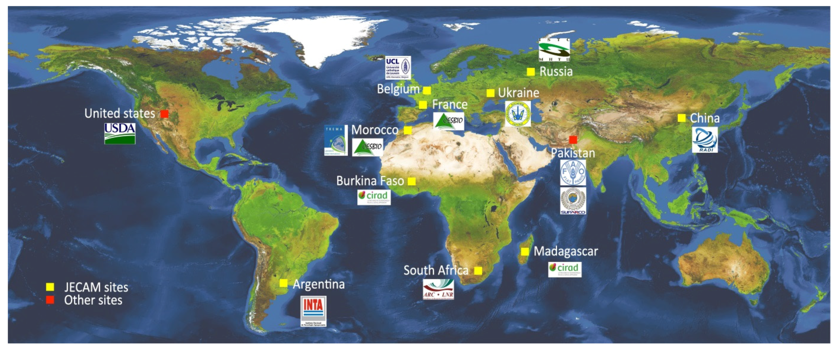
4.1. Sites Selection

The sites selection was guided by three criteria: (i) representativeness in terms of agricultural practices and climate types; (ii) availability of high spatial and temporal resolution time series; and (iii) availability of in situ data. An additional requirement expressed by ESA and confirmed by the Champion Users was to focus on Africa. As a result, 12 sites were selected (Figure 3, Table 3), making most use of the JECAM network where high spatial resolution time series were already acquired thanks to the free data access policy supported by CEOS commitment and where in situ data are collected in a systematic way.

Figure 3. Twelve globally distributed sites selected for algorithm and system design.

Figure 3. Twelve globally distributed sites selected for algorithm and system design.

Table 3. Site descriptions. In the crop description, figures in parentheses indicate the crop percentages according to FAO national statistics (first figure) and site statistics (second figure).

Spatial Extent	Main Characteristics	Main Crops and Crop Calendar
Argentina, San Antonio de Areco (JECAM)
- Top left: 33.83°S, 60.09°W - Bottom right: 34.46°S, 59.30°W	- Southern hemisphere - Temperate humid climate - Field size: 20 ha (with high variability) - Mainly rainfed crops	- Soybean (55.5%–79%), maize (11.5%–21%), wheat (9.5%–0%) - From June to December; from October to March/April
Belgium, Hesbaye (JECAM)
- Top left: 51.00° N, 4.50° E - Bottom right: 49.60° N, 5.80° E	- Northern hemisphere - Temperate climate - Field size: 3–5 ha - Mainly rainfed	- Wheat (36%–43%), maize (21%–9%), potatoes (11%–9%), sugar beet (10.5%–14%), barley (8%–9%) - From November to July; from March to September
Burkina Faso, Koumbia (JECAM)
- Top left: 11.24° N, 3.74°W - Bottom right: 10.20° N, 3.40°W	- Northern hemisphere - Tropical climate (Sudanese type) - Field size: ~1 ha	- Sorghum (32%–13.5%), cow peas (10%–9%), millet (27%–0%), maize (18%–28%), cotton (13%–38%) - From June to October
China, Shandong (JECAM)
- Top left: 37.33° N, 116.32° E - Bottom right: 36.33° N, 116.82° E	- Northern hemisphere - Temperate to semi-arid climate/monsoon climate - Field size: 0.2–0.8 ha	- Maize (20%–0%), paddy rice (17.5%–0%), wheat (14%–92%), vegetables (5%–5%) - From October to May; from June to September
France, SupdmipyOuest (JECAM)
- Top left: 44.24° N, 0.30°W - Bottom right: 43.03° N, 1.43° E	- Northern hemisphere - Temperate to Mediterranean climate - Field size: 10 ha	- Wheat (38.2%–29.5%), maize (12.5%–43%), barley (12%–0.3%), rapeseed (11.5%–6.5%), sunflower (10.5%–14%) - From October to July; from May to November
Madagascar, Antsirabe (JECAM)
- Top left: 19.38°S, 47.08°W - Bottom right: 20.01°S, 45.37°W	- Southern hemisphere - Subtropical climate - Field size: 0.03 ha - Rice cultivated with and without irrigation (terraces or basins); a lot of mixed crops	- Rice (42%–23.5%), cassava (11.5%), maize (9.5%–27%), soybean (0%–38%) - From October to April (rainy season)
Morocco, Tensift (JECAM, Centre d’Etudes Spatiales de la BIOsphère (CESBIO) and University of Cadi Ayyad, Marrakech (UCAM))
- Top left: 31.50° N, 8.24°W - Bottom right: 31.49° N, 8.22°W	- Northern hemisphere - Semi-arid climate - Field size: 0.5–40 ha - A lot of tree crops	- Wheat (41%–83%), barley (25.5%–0%), wheat-oat (0%–11%) - From December to June (winter cereals)
Pakistan (FAO with SUPARCO)
- Top left: 31.83° N, 72.26° E - Bottom right: 31.52° N, 72.69° E	- Northern hemisphere - Semi-arid to hyper-arid climate with high fluctuation in seasonal temperature regime and rainfall patterns - Field size: 0.25–6 ha	- Wheat (23%–0%), cotton (6%–12.4%), rice (6%–54.5%), maize (5%–0%), chick peas (0%–0%), sugar cane (60%–33%) - From September to May; from May to December
Russia, Tula (JECAM)
- Top left: 53.67° N, 37.14° E - Bottom right: 53.59° N, 37.33° E	- Northern hemisphere - Moderate continental climate - Field size: 50–120 ha - Only rainfed crops	- Wheat (40.5%–45.5%), barley (14.6%–24.5%), sunflower (12%–4.5%), oats (5.5%–0%), rapeseed (1%–17.5%) - From September to July
South Africa, Freestate (JECAM)
- Top left: 26.85°S, 24.55° E - Bottom right: 30.74°S, 29.77° E	- Southern hemisphere - Sub-humid to semi-arid climate - Field size: 40 ha	- Maize (53%–88%), wheat (8.5%–0%), sunflower (8.5%–9%), soybean (8%–2%) - From December to June; from April to November
Ukraine, Phenichne and Velyka Snitynka (JECAM)
- Top left: 50.14° N, 29.96° E - Bottom right: 50.01° N, 30.26° E	- Northern hemisphere - Humid continental climate, with snow cover in February and March - Field size: 30–250 ha	- Wheat (23%–22%), sunflower (20.5%–10.2%), maize (18%–36.5%), barley (13.5%–0%), potatoes (6%–0%), soybean (1%–17%) - From September to July; from April to October
United States, Maricopa (USDA)
- Top left: 33.41° N, 112.71°W - Bottom right: 32.59° N, 111.19°W	- Northern hemisphere - Long hot summers and cool-warm winter - Field sizes: 20–120 ha - Irrigated agriculture	- Maize (34.5%–13.5%), soybean (30%–0%), wheat (19.5%–1.5%), alfalfa (0%–44.5%), cotton (0%–18.5%), barley (1%–13.5%) - From November to May; from March to September; all year round for alfalfa

Table 3. Site descriptions. In the crop description, figures in parentheses indicate the crop percentages according to FAO national statistics (first figure) and site statistics (second figure).

Spatial Extent	Main Characteristics	Main Crops and Crop Calendar
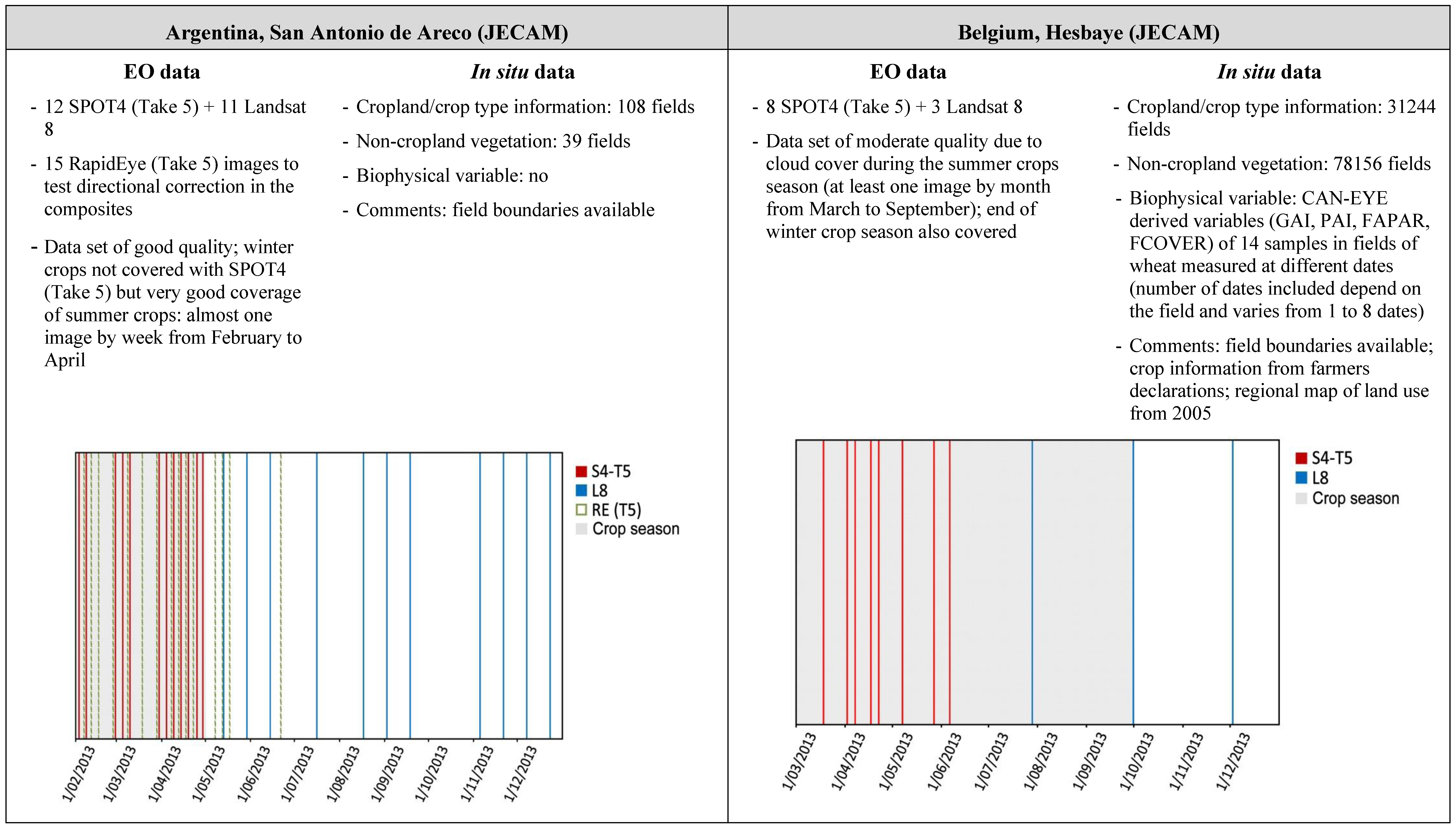
Argentina, San Antonio de Areco (JECAM)
- Top left: 33.83°S, 60.09°W - Bottom right: 34.46°S, 59.30°W	- Southern hemisphere - Temperate humid climate - Field size: 20 ha (with high variability) - Mainly rainfed crops	- Soybean (55.5%–79%), maize (11.5%–21%), wheat (9.5%–0%) - From June to December; from October to March/April
Belgium, Hesbaye (JECAM)
- Top left: 51.00° N, 4.50° E - Bottom right: 49.60° N, 5.80° E	- Northern hemisphere - Temperate climate - Field size: 3–5 ha - Mainly rainfed	- Wheat (36%–43%), maize (21%–9%), potatoes (11%–9%), sugar beet (10.5%–14%), barley (8%–9%) - From November to July; from March to September
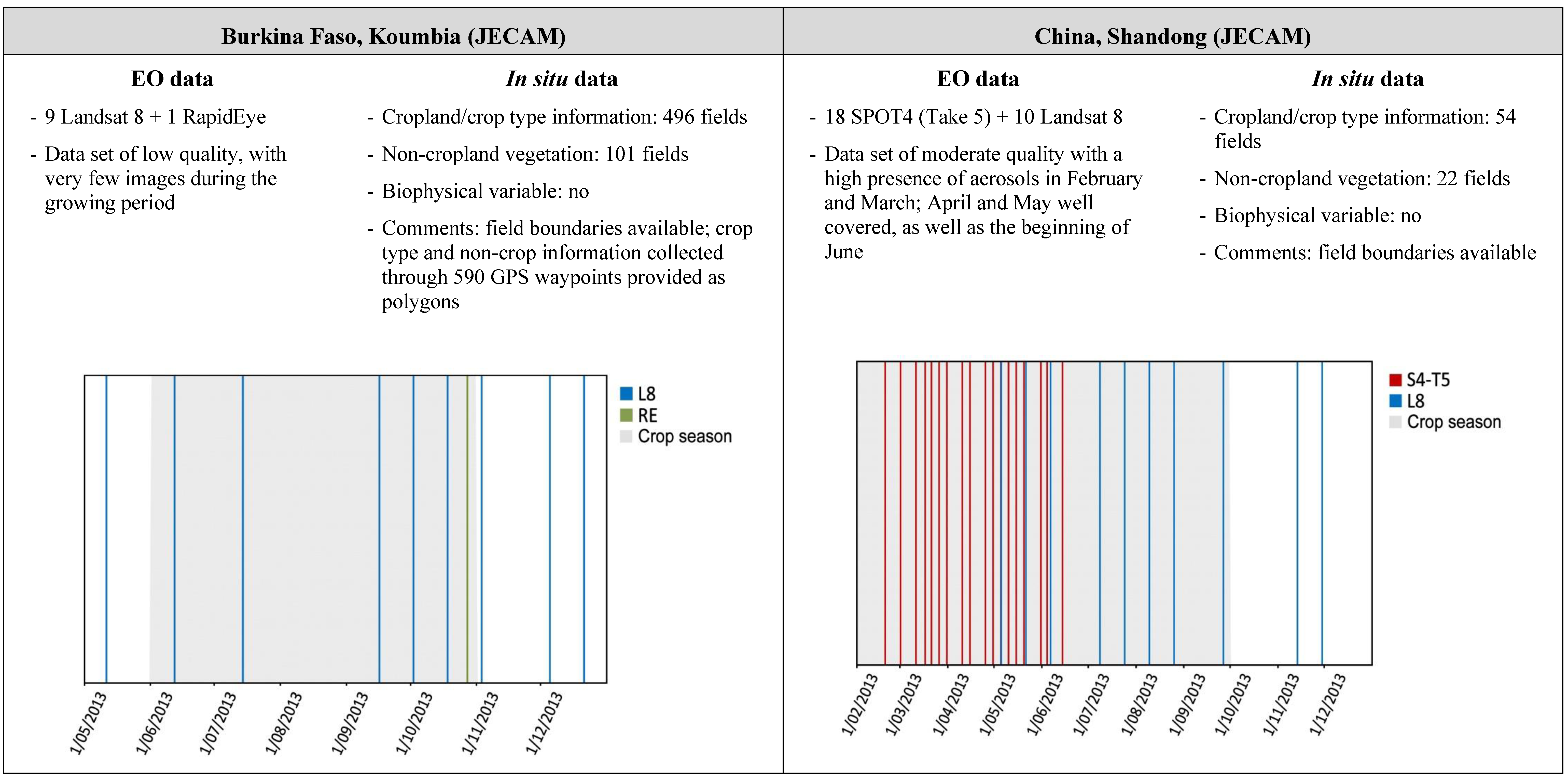
Burkina Faso, Koumbia (JECAM)
- Top left: 11.24° N, 3.74°W - Bottom right: 10.20° N, 3.40°W	- Northern hemisphere - Tropical climate (Sudanese type) - Field size: ~1 ha	- Sorghum (32%–13.5%), cow peas (10%–9%), millet (27%–0%), maize (18%–28%), cotton (13%–38%) - From June to October
China, Shandong (JECAM)
- Top left: 37.33° N, 116.32° E - Bottom right: 36.33° N, 116.82° E	- Northern hemisphere - Temperate to semi-arid climate/monsoon climate - Field size: 0.2–0.8 ha	- Maize (20%–0%), paddy rice (17.5%–0%), wheat (14%–92%), vegetables (5%–5%) - From October to May; from June to September
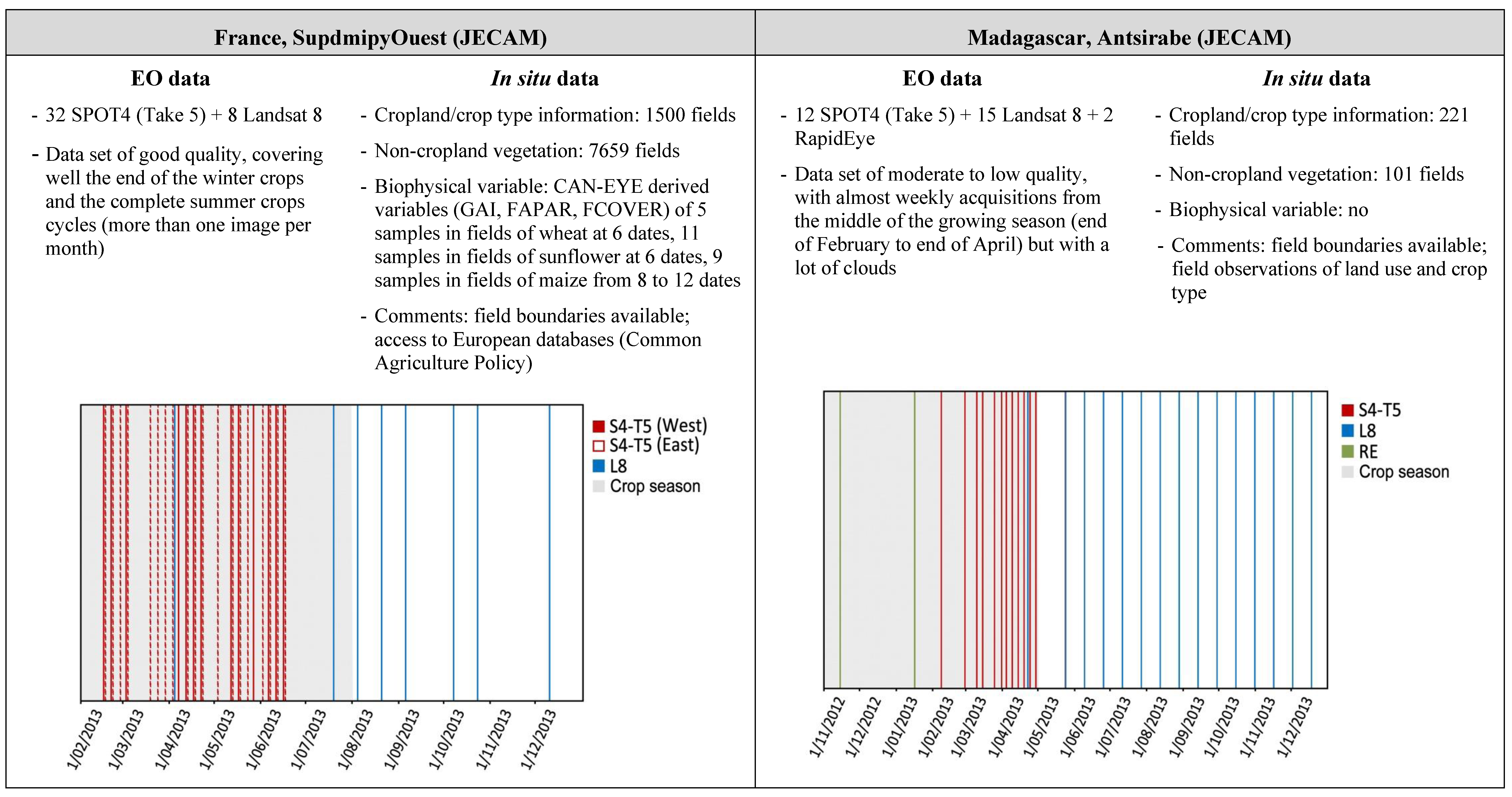
France, SupdmipyOuest (JECAM)
- Top left: 44.24° N, 0.30°W - Bottom right: 43.03° N, 1.43° E	- Northern hemisphere - Temperate to Mediterranean climate - Field size: 10 ha	- Wheat (38.2%–29.5%), maize (12.5%–43%), barley (12%–0.3%), rapeseed (11.5%–6.5%), sunflower (10.5%–14%) - From October to July; from May to November
Madagascar, Antsirabe (JECAM)
- Top left: 19.38°S, 47.08°W - Bottom right: 20.01°S, 45.37°W	- Southern hemisphere - Subtropical climate - Field size: 0.03 ha - Rice cultivated with and without irrigation (terraces or basins); a lot of mixed crops	- Rice (42%–23.5%), cassava (11.5%), maize (9.5%–27%), soybean (0%–38%) - From October to April (rainy season)
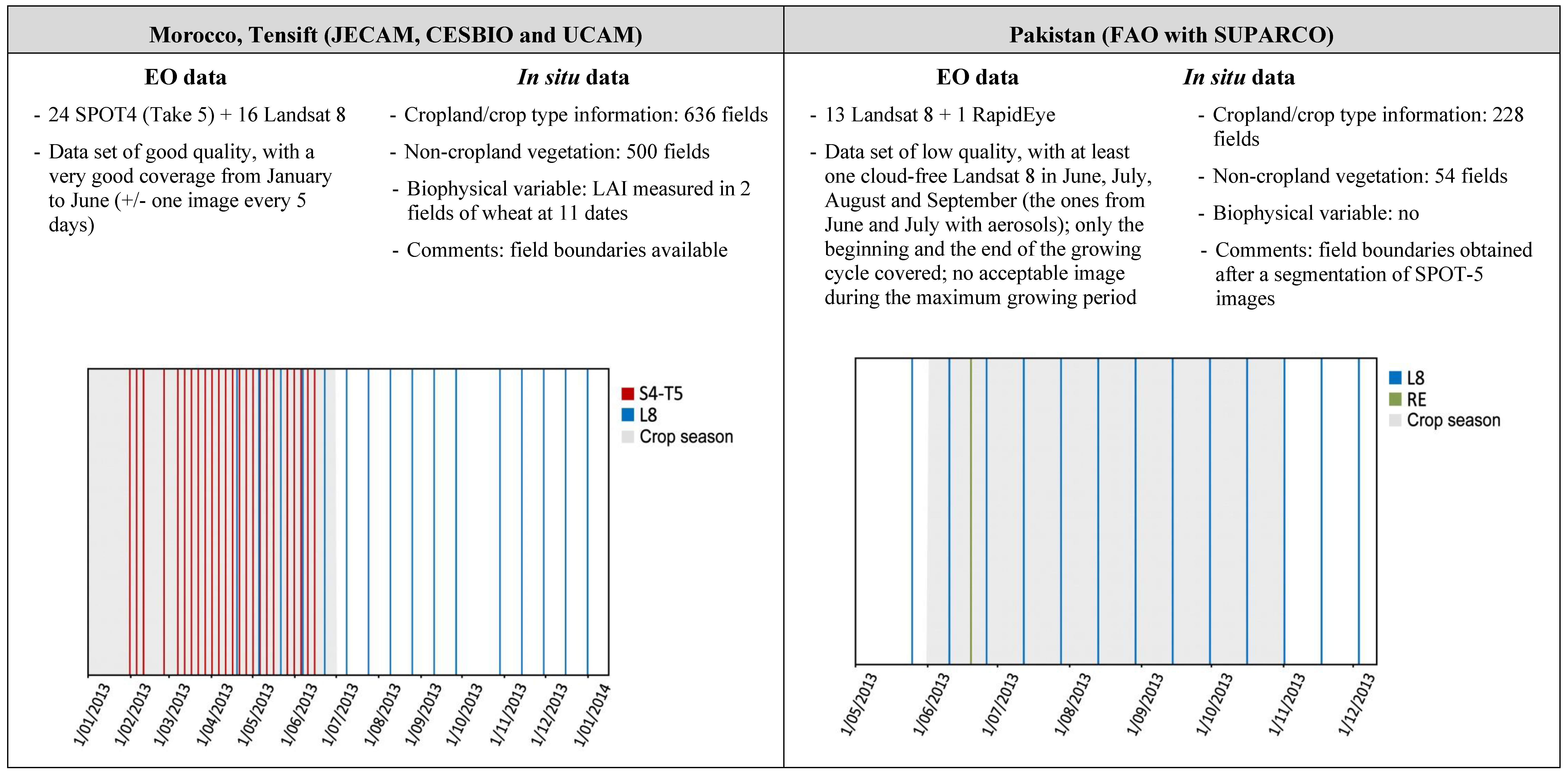
Morocco, Tensift (JECAM, Centre d’Etudes Spatiales de la BIOsphère (CESBIO) and University of Cadi Ayyad, Marrakech (UCAM))
- Top left: 31.50° N, 8.24°W - Bottom right: 31.49° N, 8.22°W	- Northern hemisphere - Semi-arid climate - Field size: 0.5–40 ha - A lot of tree crops	- Wheat (41%–83%), barley (25.5%–0%), wheat-oat (0%–11%) - From December to June (winter cereals)
Pakistan (FAO with SUPARCO)
- Top left: 31.83° N, 72.26° E - Bottom right: 31.52° N, 72.69° E	- Northern hemisphere - Semi-arid to hyper-arid climate with high fluctuation in seasonal temperature regime and rainfall patterns - Field size: 0.25–6 ha	- Wheat (23%–0%), cotton (6%–12.4%), rice (6%–54.5%), maize (5%–0%), chick peas (0%–0%), sugar cane (60%–33%) - From September to May; from May to December
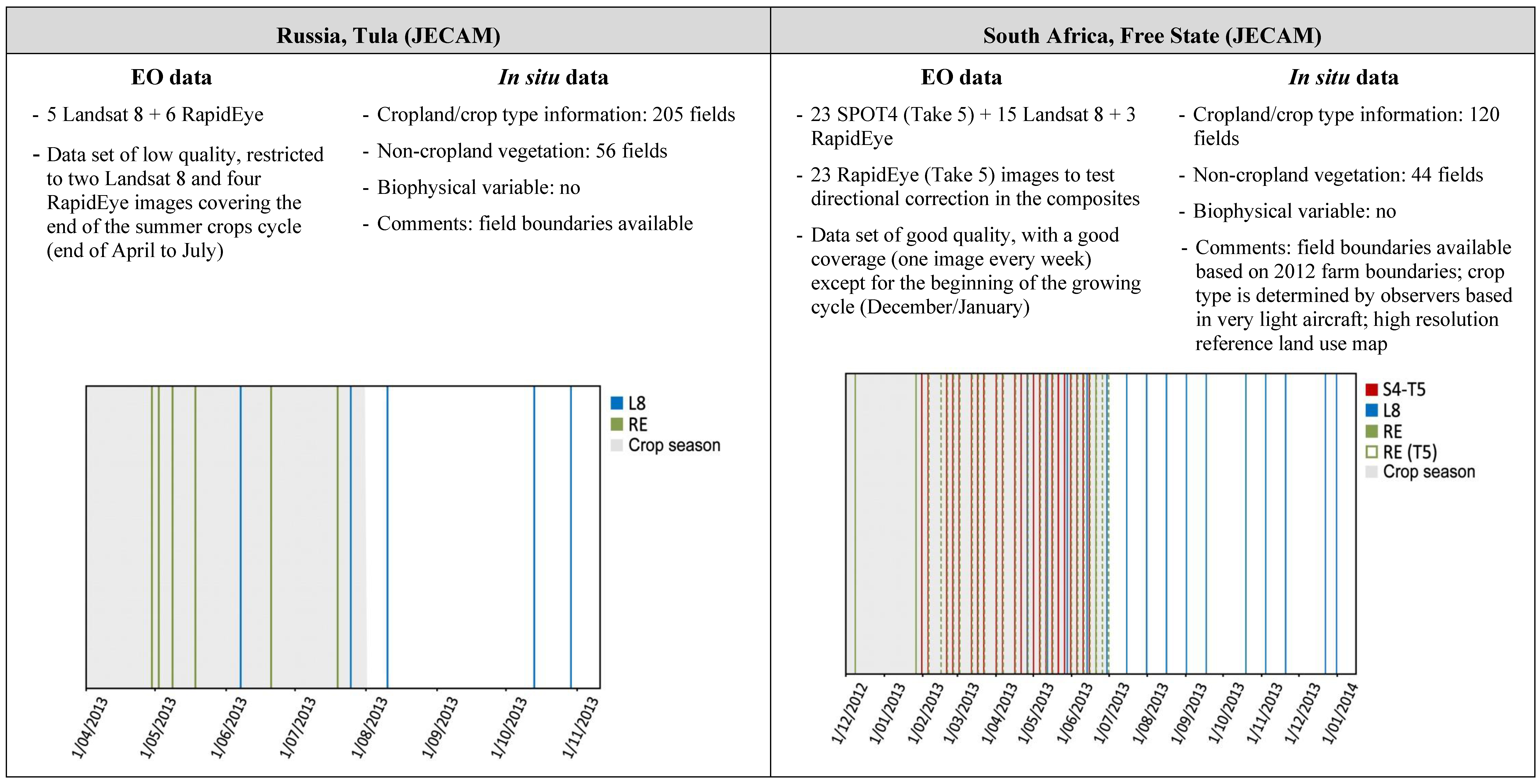
Russia, Tula (JECAM)
- Top left: 53.67° N, 37.14° E - Bottom right: 53.59° N, 37.33° E	- Northern hemisphere - Moderate continental climate - Field size: 50–120 ha - Only rainfed crops	- Wheat (40.5%–45.5%), barley (14.6%–24.5%), sunflower (12%–4.5%), oats (5.5%–0%), rapeseed (1%–17.5%) - From September to July
South Africa, Freestate (JECAM)
- Top left: 26.85°S, 24.55° E - Bottom right: 30.74°S, 29.77° E	- Southern hemisphere - Sub-humid to semi-arid climate - Field size: 40 ha	- Maize (53%–88%), wheat (8.5%–0%), sunflower (8.5%–9%), soybean (8%–2%) - From December to June; from April to November
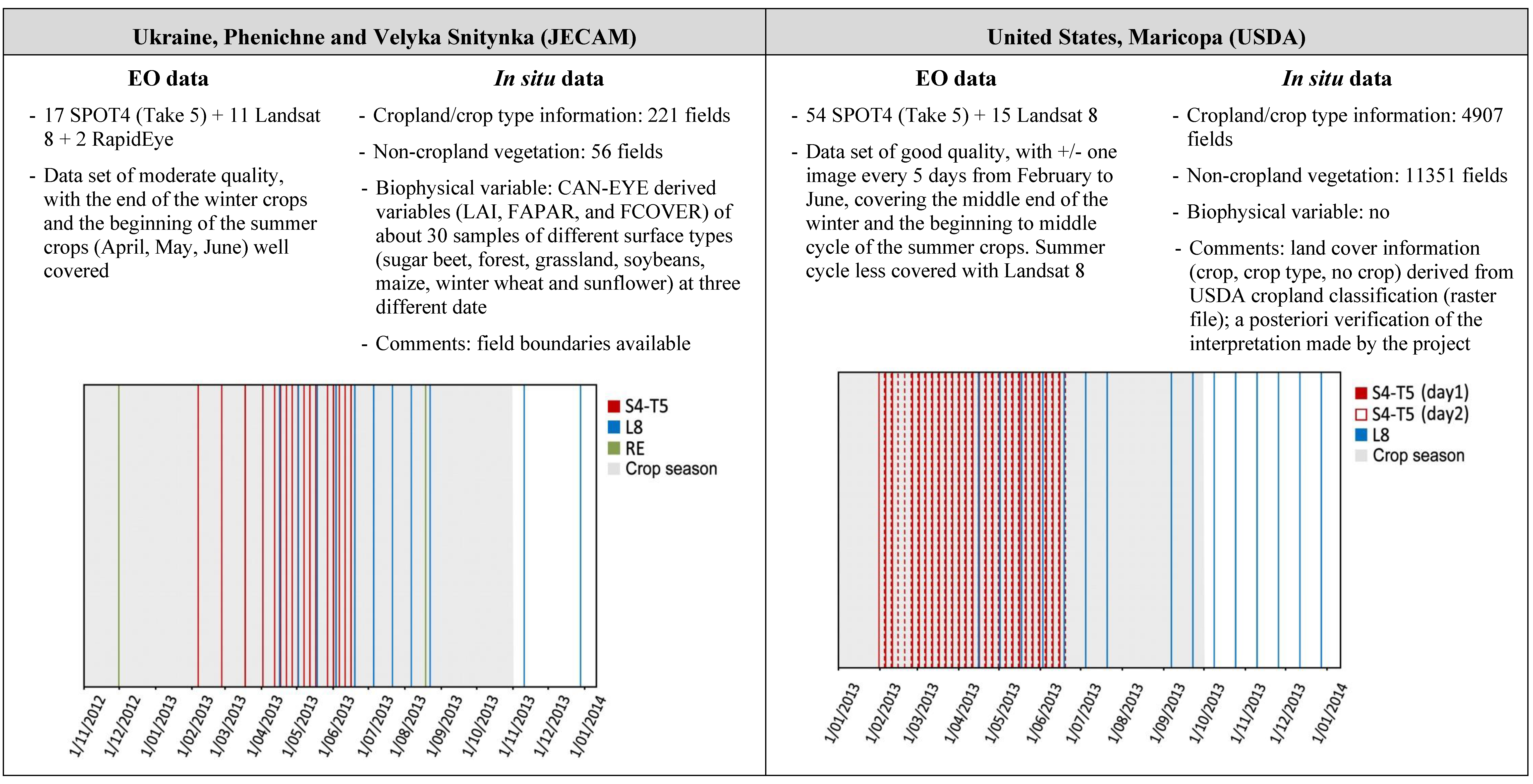
Ukraine, Phenichne and Velyka Snitynka (JECAM)
- Top left: 50.14° N, 29.96° E - Bottom right: 50.01° N, 30.26° E	- Northern hemisphere - Humid continental climate, with snow cover in February and March - Field size: 30–250 ha	- Wheat (23%–22%), sunflower (20.5%–10.2%), maize (18%–36.5%), barley (13.5%–0%), potatoes (6%–0%), soybean (1%–17%) - From September to July; from April to October
United States, Maricopa (USDA)
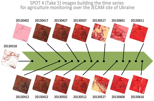
- Top left: 33.41° N, 112.71°W - Bottom right: 32.59° N, 111.19°W	- Northern hemisphere - Long hot summers and cool-warm winter - Field sizes: 20–120 ha - Irrigated agriculture	- Maize (34.5%–13.5%), soybean (30%–0%), wheat (19.5%–1.5%), alfalfa (0%–44.5%), cotton (0%–18.5%), barley (1%–13.5%) - From November to May; from March to September; all year round for alfalfa

This selection tackles a large variety of climate types and agricultural practices. It also includes sites in the southern and northern hemispheres as well as in temperate, Mediterranean and tropical regions, which will allow distributing the workload along the year and learning from one site to the other.

4.2. EO Data

4.2.1. Selection

Three sensors were considered to build the EO time series: SPOT 4, Landsat 8 and RapidEye. Characteristics of these three sensors are described in Table 4.

SPOT 4 images were those acquired by the SPOT4 (Take 5) experiment which took place between February and June 2013 [18]. Priority was given to this SPOT4 (Take 5) data set, as it aimed to provide time series of optical images simulating the periodicity, the resolution and the large swath of Sentinel-2. Landsat 8 images (with less than 70% of cloud cover) were then considered as a complement to increase the temporal resolution of the SPOT4 (Take 5) time series and the time period covered by the time series when relevant. Finally, RapidEye data were selected only over specific sites during specific periods when there were no SPOT4 (Take 5) or Landsat 8 data. Images with high cloud coverage (above 50%) were marked as less appropriate.

4.2.2. Pre-Processing

The SPOT4 (Take 5) data were made available as L2A products (see Table 4). The reader is referred to [18] for the details of the SPOT4 (Take 5) pre-processing methodology and validation. One particularity of the methodology comes from the Multisensor Atmospheric Correction and Cloud Screening (MACCS) processor, which uses multi-temporal criteria to build the various masks and to detect the aerosols before the atmospheric correction [37,38,39].

Landsat 8 data were acquired at level L1T (see Table 4) in the UTM projection from the Earth Explorer website [40]. They were pre-processed at their original spatial resolution to L2A using nearly the same method as the one developed for the SPOT4 (Take 5) images, thus also involving the MACCS processor [41]. The processing was slightly enriched compared to the SPOT4 (Take 5) since additional bands were available: band 9 (cirrus band) enabled an enhanced detection of high and thin clouds and band 2 provided an additional criterion to detect aerosols. L2A products were generated for the visible, near-infrared and shortwave infrared bands (bands 1 to 7). The thermal bands were not processed, as they are not available on Sentinel-2.

RapidEye data were acquired as L3A products (see Table 4) [42]. After a resampling to the Sentinel-2 10 m resolution, they were processed to L3A BOA (see Table 4). In this case, the processing was slightly different since the multi-temporal method implemented in MACCS requires data acquired under constant viewing angles, which is not the case for the RapidEye sensor. The cloud detection was performed through a semi-automatic approach based on a Supervised Vector Machine active learning algorithm embedded into a QGIS plugin. The cloud shadows were then retrieved assuming a constant cloud altitude within the image and by searching the ground displacement for the best match with decreased reflectance values due to shadows. The Aerosol Optical Thickness (AOT) estimation relied on the Dark Dense Vegetation method available in MACCS and described in [43].

Table 4. Characteristics of the three sensors used to build the EO time series. For the sake of comparison, Sentinel-2 main characteristics are also detailed.

	SPOT 4	Landsat 8	RapidEye	Sentinel-2
Spatial resolution	20 m	30 m	6.5 m (resampled to 5 m)	10, 20, 60 m
Field of view	60 to 120 km	180 km	77 km	290 km
Repeat period	5 days	16 days	Daily (off-nadir)/5.5 days (at nadir)	5 days (with 2 sensors)
Time Period	February 2013–June 2013	April 2013–present	September 2008–present	From June 2015
Bands	- B1: 0.50–0.59 µm - B2: 0.61–0.68 µm - B3: 0.78–0.89 µm - B4: 1.58–1.75 µm	- B1: 0.43–0.45 µm - B2: 0.45–0.51 µm - B3: 0.53–0.59 µm - B4: 0.64–0.67 µm - B5: 0.85–0.88 µm - B6: 1.57–1.65 µm - B7: 2.11–2.29 µm - B9: 1.36–1.38 µm - B10: 10.60–11.19 µm - B11: 11.50–12.51 µm	- B1: 0.44–0.51 µm - B2: 0.52–0.59 µm - B3: 0.63–0.685 µm - B4: 0.69–0.73 µm - B5: 0.76–0.85 µm	- B1: 0.433–0.453 µm - B2: 0.4575–0.5225 µm - B3: 0.5425–0.5775 µm - B4: 0.65–0.68 µm - B5: 0.6975–0.7125 µm - B6: 0.7325–0.7475 µm - B7: 0.773–0.793 µm - B8: 0.7845–0.8995 µm - B8a: 0.855–0.875 µm - B9: 0.935–0.955 µm - B10: 1.365–1.395 µm - B11: 1.565–1.655 µm - B12: 2.1–2.28 µm
Products used in the TDS	Input and output	Input	Input	/
	Level 2A (L2A): surface reflectance values (top of canopy) with masks for clouds, cloud shadows, snow and water
			Level 3A (L3A): surface reflectance values (top of canopy) with radiometric, sensor and geometric correction
		Level 1T (L1T): surface reflectance values (top of atmosphere) with masks for clouds, cloud shadows, snow, water and level of aerosol
		Output	Output:	/
			Level 3A Bottom of Atmosphere (L3A BOA): surface reflectance values with masks for clouds and water
		L2A

Table 4. Characteristics of the three sensors used to build the EO time series. For the sake of comparison, Sentinel-2 main characteristics are also detailed.

	SPOT 4	Landsat 8	RapidEye	Sentinel-2
Spatial resolution	20 m	30 m	6.5 m (resampled to 5 m)	10, 20, 60 m
Field of view	60 to 120 km	180 km	77 km	290 km
Repeat period	5 days	16 days	Daily (off-nadir)/5.5 days (at nadir)	5 days (with 2 sensors)
Time Period	February 2013–June 2013	April 2013–present	September 2008–present	From June 2015
Bands	- B1: 0.50–0.59 µm - B2: 0.61–0.68 µm - B3: 0.78–0.89 µm - B4: 1.58–1.75 µm	- B1: 0.43–0.45 µm - B2: 0.45–0.51 µm - B3: 0.53–0.59 µm - B4: 0.64–0.67 µm - B5: 0.85–0.88 µm - B6: 1.57–1.65 µm - B7: 2.11–2.29 µm - B9: 1.36–1.38 µm - B10: 10.60–11.19 µm - B11: 11.50–12.51 µm	- B1: 0.44–0.51 µm - B2: 0.52–0.59 µm - B3: 0.63–0.685 µm - B4: 0.69–0.73 µm - B5: 0.76–0.85 µm	- B1: 0.433–0.453 µm - B2: 0.4575–0.5225 µm - B3: 0.5425–0.5775 µm - B4: 0.65–0.68 µm - B5: 0.6975–0.7125 µm - B6: 0.7325–0.7475 µm - B7: 0.773–0.793 µm - B8: 0.7845–0.8995 µm - B8a: 0.855–0.875 µm - B9: 0.935–0.955 µm - B10: 1.365–1.395 µm - B11: 1.565–1.655 µm - B12: 2.1–2.28 µm
Products used in the TDS	Input and output	Input	Input	/
	Level 2A (L2A): surface reflectance values (top of canopy) with masks for clouds, cloud shadows, snow and water
			Level 3A (L3A): surface reflectance values (top of canopy) with radiometric, sensor and geometric correction
		Level 1T (L1T): surface reflectance values (top of atmosphere) with masks for clouds, cloud shadows, snow, water and level of aerosol
		Output	Output:	/
			Level 3A Bottom of Atmosphere (L3A BOA): surface reflectance values with masks for clouds and water
		L2A

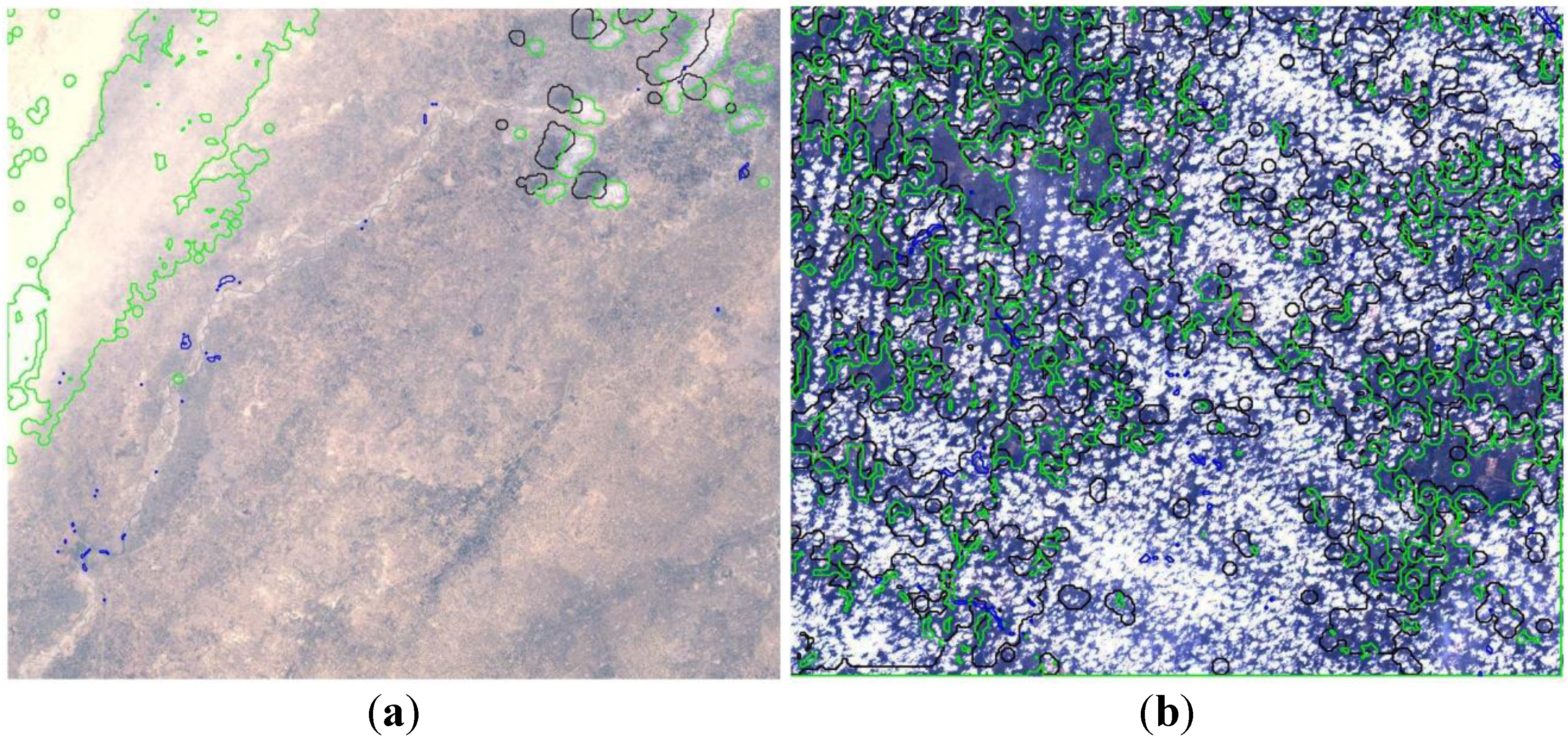
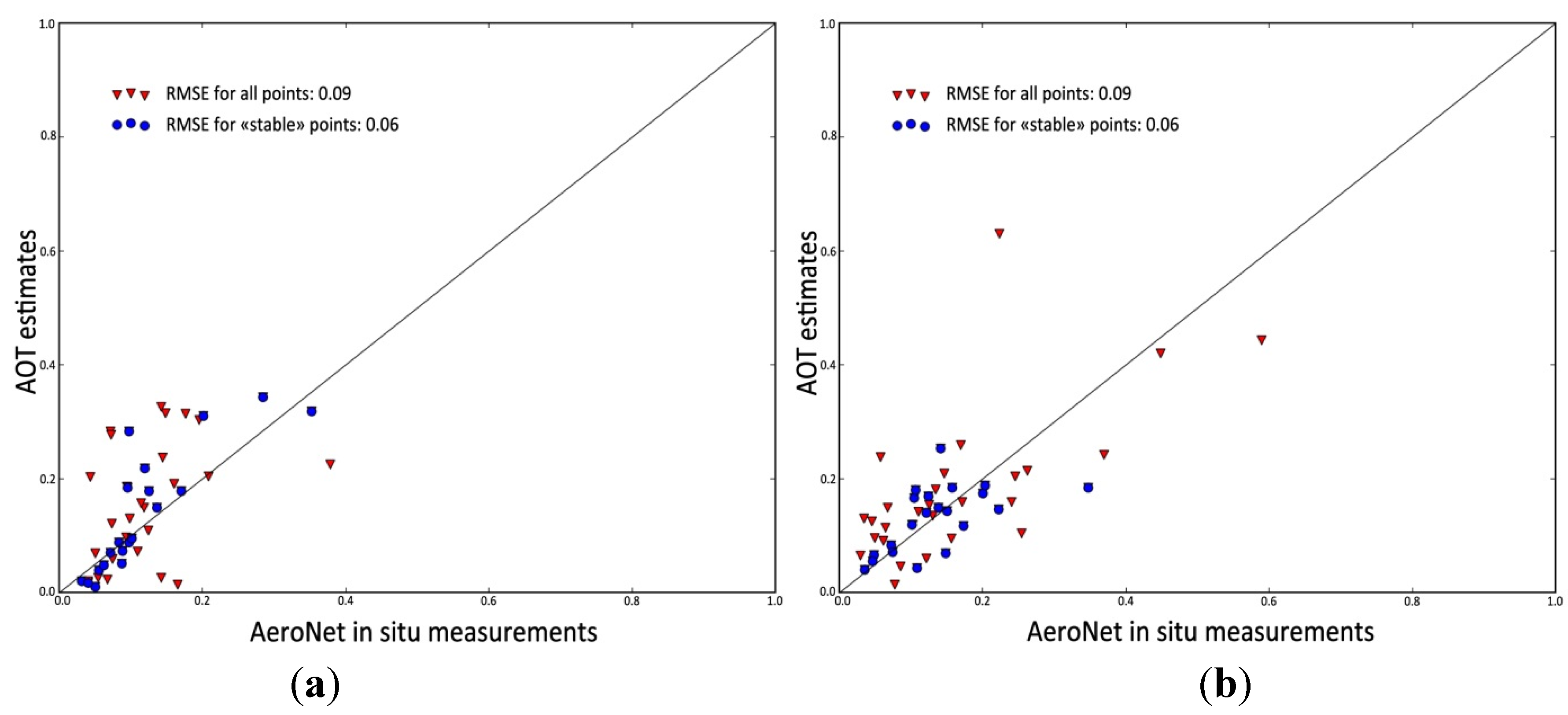
4.2.3. Quality Assessment

The quality of the resulting L2A time series was assessed, looking at several properties: (i) the geometry and the co-registration of the images over time and between sensors; (ii) the cloud masks; (iii) the aerosol estimates; and (iv) the temporal consistency of the surface reflectance values.

• Geometry

The geometry of the SPOT4 (Take 5) data set is fully documented in [18]. Given that the initial geolocation error could reach 1500 m, the multi-temporal registration was qualified as good. For most images, 50% of the measurements show that the registration performance is better than 0.3 pixel (6.66 m) and for 80% of the measurements, it is better than 0.5 pixel (10 m).

The geometric performance of the Landsat 8 L1T products is detailed in [44]. The measured band-to-band registration accuracy exceeds the requirement threshold for all band-pair combinations and greatly exceeds the threshold for all band-pairs that do not include the cirrus band. As for image-to-image registration accuracy, the performance was found again to exceed the requirement of 12 meters in the line and sample directions: 3.052 and 2.250 meters in the line and sample directions respectively for the all validation sample and 6.623 and 5.051 meters in the line and sample directions for the worst image of the samples. These generally good results were confirmed in the TDS, except for the French site where a 38-m bias was found. In this particular case, the image was nearly completely covered by clouds, resulting in few ground control points.

As for the RapidEye sensor, all images are provided with a guaranteed minimum geometric accuracy of 30.34 m [42]. These specifications were already confirmed in the literature [45,46] and were largely met in the TDS.

The multi-temporal registration of all sensors was also qualitatively assessed: pixels corresponding to borders between two different surface types were selected for each sensor and site and the temporal profile of each reflectance band was analyzed. When a significant difference between the expected reflectance value and the observed one was detected, the two consecutive images were visually analyzed. The analysis resulted in very good geometric accuracy for all data sets. When an anomaly was observed, it was mainly due to undetected clouds or shadows, but also to seasonality or changes in the brightness that were not related to the co-registration.

Finally, the geometric consistency between images acquired by different sensors was analyzed. In general, the images of the different sensors were properly aligned. The geometric consistency between the SPOT4 (Take 5) and Landsat 8 images was naturally ensured since the SPOT4 (Take 5) ortho-rectification used the Landsat 8 images as reference for all sites. The only exception is the French site as already mentioned. The consistency of the RapidEye data set with SPOT4 (Take 5) and Landsat 8 images was quantified (Table 5). The figures were obtained through a set of 90 points for the SPOT4 (Take 5) analysis and a set of 116 points for the Landsat 8 analysis. In both cases, the points were spread over all the RapidEye images (between 2 and 5 points by image). The results are below the SPOT4 (Take 5) and the Landsat 8 pixel resolution, which means that the three data sets could be used together.

Table 5. Geometric consistency of the RapidEye data set with SPOT4 (Take 5) and Landsat 8 images.

SPOT4 (Take 5)		Landsat 8
RMSEx	RMSEy	RMSEx	RMSEy
11.3 m	19.4 m	13.4 m	15.1m

Table 5. Geometric consistency of the RapidEye data set with SPOT4 (Take 5) and Landsat 8 images.

SPOT4 (Take 5)		Landsat 8
RMSEx	RMSEy	RMSEx	RMSEy
11.3 m	19.4 m	13.4 m	15.1m

• Cloud masks

The quality of the SPOT4 (Take 5) cloud masks was assessed outside of this project. The protocol and the results are documented in [18]. The evaluation of the clouds and cloud shadows masks relied on a visual verification of quick-looks. In spite of some imperfections, even very thin clouds and their shadows were usually detected.

The quality of the cloud masks generated for the Landsat 8 and RapidEye data was assessed also by visual inspection. In general, for the two sensors, the performance of the cloud screening is good, even if some problems were noticed when dealing with small clouds. When working with Landsat 8 data, clouds identification is slightly improved when using the additional spectral information provided by the cirrus band 9. Figure 4a provides an example of cloud detection on Landsat 8 data over the Pakistan site. This is a good example of the interest of a multi-temporal method (as implemented in MACCS) for cloud detection. A method based on reflectance thresholds would classify the desert (North West corner) as a cloud, or miss the haze in the valley close to desert or the clouds in the top right of image. Here, haze, clouds and their shadows were very well detected. Some possible false detections may be observed over the desert because it was a drying period at the beginning of summer. Despite the very high AOT during image acquisition, no other false detection of clouds was observed.

Figure 4. Cloud detection (a) over the Pakistan site (May 25, 2013, top left: 31.74°N–72.46°E, low right: 31.52°N–72.70°E) with haze and clouds over desert and (b) over the Ukrainian site (November 10, 2013, top left: 50.25° N–29.80° E, low right: 49.69° N–30.71°E) with a large number of cumulus clouds. Clouds are circled in green and shadows in black.

Figure 4. Cloud detection (a) over the Pakistan site (May 25, 2013, top left: 31.74°N–72.46°E, low right: 31.52°N–72.70°E) with haze and clouds over desert and (b) over the Ukrainian site (November 10, 2013, top left: 50.25° N–29.80° E, low right: 49.69° N–30.71°E) with a large number of cumulus clouds. Clouds are circled in green and shadows in black.

This good performance of the cloud mask could be even better by further improving the mask expansion process. Currently, the final mask is provided after an expansion of 480 meters in all directions, which is justified for clouds with fuzzy edges as illustrated in Figure 4b. In this case, the expansion fills the gaps between clouds in which the surface reflectance values would be affected by shadows and by the light reflected by clouds. Yet, in the case of scattered cumulus clouds which usually have sharp edges, a 480 meters expansion tends to exaggerate the size of the clouds.

• Aerosol estimates

The aerosol estimates were validated for the whole SPOT4 (Take 5) experiment (Figure 5a from [18]). They were compared with in situ measurements from the Aeronet Network [47] if available and if not, the estimates at 550 nm were compared to the Aeronet level 2 data. All the Aeronet sites which were within 50 km from the image were used.

The standard deviation of the AOT estimates was 0.09. It reduced to 0.06 when removing the Aeronet data that were likely corrupted by the presence of clouds. The criteria used for this screening are defined in [18]: only cloud-free images (i.e., for which there should be less than 10% of clouds in a 20-km neighborhood from the Aeronet site) and Aeronet observations which are stable over time (i.e., below 0.02 within an hour around the satellite overpass time) are kept. These conditions correspond to the stable condition in the legend of Figure 5, represented by blue circles. The highest disagreements were observed for the Tunisian site, which is not part of the project. The standard deviations for the Sen2-Agri sites were less than 0.06.

Figure 5. Validation of AOT estimates at 550 nm determined for (a) SPOT4 (Take 5) images (from [18]) and (b) Landsat 8 images using Aeronet in situ measurements.

Figure 5. Validation of AOT estimates at 550 nm determined for (a) SPOT4 (Take 5) images (from [18]) and (b) Landsat 8 images using Aeronet in situ measurements.

The same assessment was performed for the Landsat 8 data (Figure 5b). The Aeronet sites that were used are: Seysses, Le Fauga and Avignon in France; Kyiv in Ukraine and Saada and Ouarzazate in Morocco. Here again, the accuracy of aerosol estimates was excellent. Despite the reduced overpass frequency offered by Landsat sensors (16 vs. 5 days), the same level of accuracy is obtained as for the SPOT4 (Take 5) data set.

Unfortunately, no Aeronet sites were available near the Chinese and Pakistani sites where very large AOT were observed. For 2013, mean AOT values at 500 nm of 0.719 and of 0.706 were measured by the closest photometers of Lahore (Pakistan) and Beijing (China), respectively [48,49]. These figures must be taken cautiously as the photometers are at a significant distance from the agricultural sites and are located in cities. In Pakistan, the estimations are more or less representative while in China, they are slightly lower (around 0.5). Consequently, atmospheric corrections over these sites were less accurate and added noise to the surface reflectance time series.

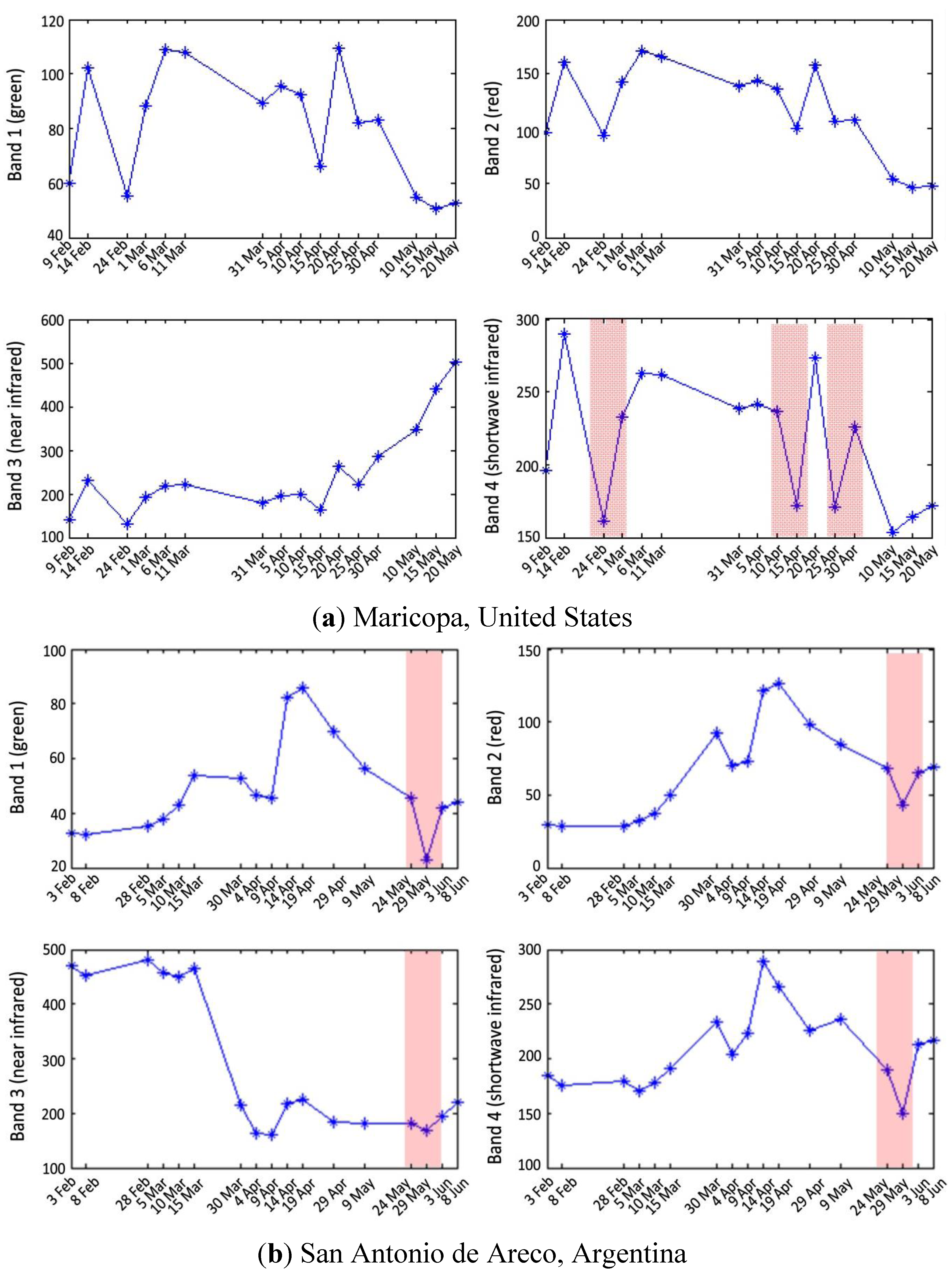
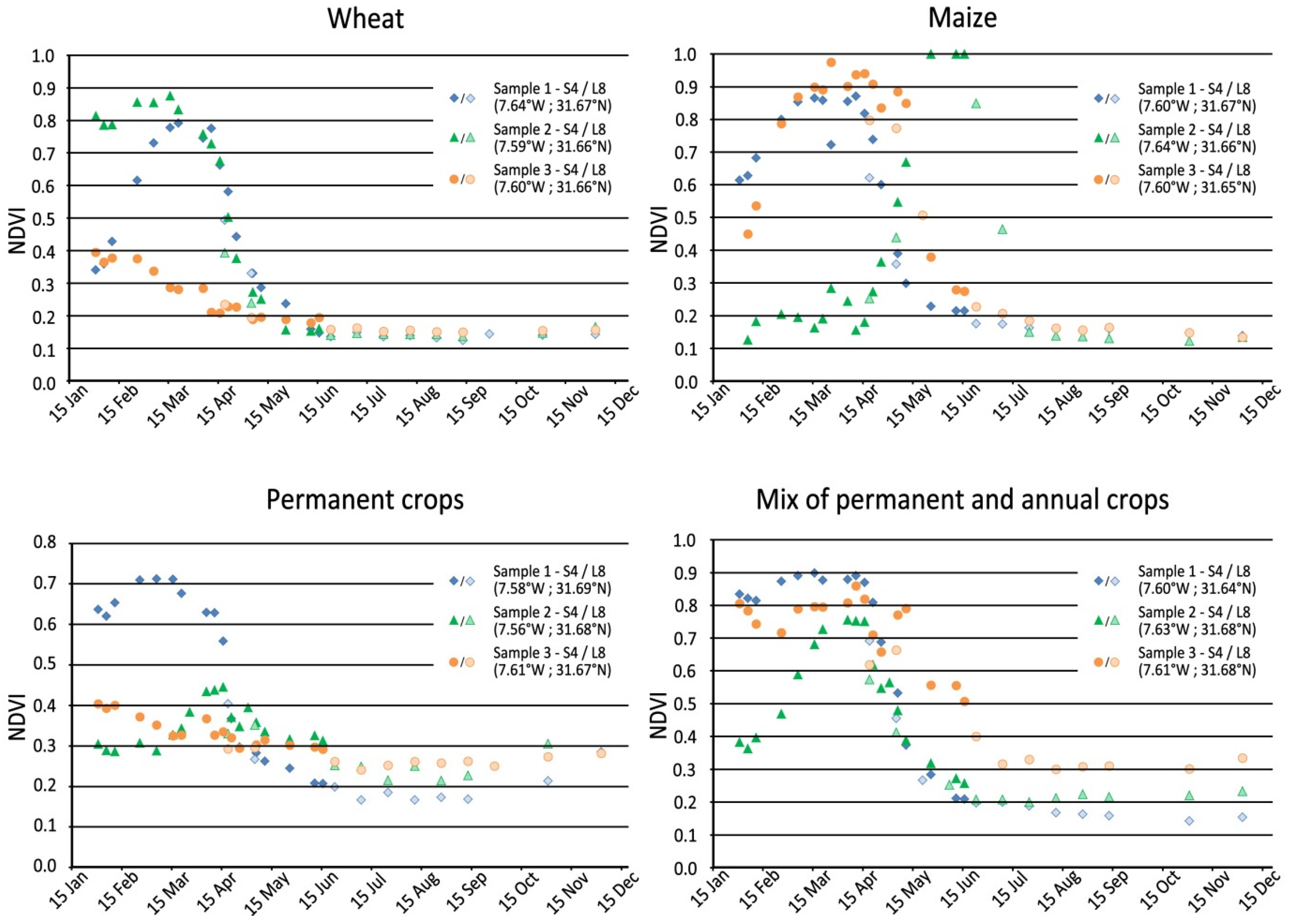
• Temporal consistency of surface reflectance values

The temporal consistency of the TDS was assessed by visually analyzing the temporal profiles of the individual reflectance bands and of the NDVI coming from different agricultural fields. When unexpected reflectance values were observed in the profiles, the images were visually checked. This analysis was done per site for each sensor, looking at the temporal profiles coming from the average of all pixels belonging to one field.

In general, the detected outliers were explained by undetected clouds or shadows, the presence of aerosols, etc. Two issues were noticed in the SPOT4 (Take 5) data sets of Maricopa (United States) and San Antonio de Areco (Argentina), which could be explained by irrigation events (Figure 6). In the case of Maricopa, irrigation explained variations observed in the band 4 (shortwave infrared) for the dates of 15, 20 and 25 April. The same occurred over the Argentinian image of May 29 when the reflectance values in the bands 1, 2 and 3 (green, red, near infrared) dropped in an unexpected way (up to 50% for the bands1 and 2).

Figure 6. Temporal profiles in the four spectral bands of the SPOT4 (Take 5) time series over the (a) American and (b) Argentinian sites. Irrigation periods are highlighted in red.

Figure 6. Temporal profiles in the four spectral bands of the SPOT4 (Take 5) time series over the (a) American and (b) Argentinian sites. Irrigation periods are highlighted in red.

Finally, the temporal consistency of the reflectance values between sensors (SPOT4 (Take 5) and Landsat 8) was evaluated, for the sites of France, Morocco and Belgium. Landsat 8 data were resampled to 20 meters and the same methodology as before was applied, thus analyzing temporal profiles made of two sensors. The conclusion was that the profiles coming from the two sensors were coherent and temporally consistent, as shown in Figure 7 for the Moroccan site.

Figure 7. NDVI temporal profiles from parcels of wheat, maize, permanent crops and mix of permanent and annual crops over the Moroccan site. For each crop, temporal profiles of three parcels are provided, plain and hatched dots showing NDVI values obtained from SPOT4 (Take 5) and Landsat 8 images respectively.

Figure 7. NDVI temporal profiles from parcels of wheat, maize, permanent crops and mix of permanent and annual crops over the Moroccan site. For each crop, temporal profiles of three parcels are provided, plain and hatched dots showing NDVI values obtained from SPOT4 (Take 5) and Landsat 8 images respectively.

4.3. In Situ Data Collection and Formatting

In situ data for algorithm development and products validation were collected for the year 2013 by the team(s) responsible of each site. All site managers agreed to share their data with the project. Except for Belgium (where an official land cover database was already available for 2013) and United States (where annual cropland classifications exist as raster files), the cropland data (crop presence and crop type identification) were obtained by field observations during the main growing season of the year 2013. In order to have a complete data set allowing a proper validation of the cropland products, non-cropland classes were also requested and obtained either from field observations or from institutional data. Regarding the biophysical variables, only 4 sites had these kinds of data: Belgium, France, Morocco and Ukraine. Over Belgium, France and Ukraine, LAI was obtained using the CAN-EYE imaging software [50] which extracts canopy structure characteristics from true-color images either acquired with a fish-eye or with a classic objective. Over Morocco, LAI was also estimated from hemispheric images using a MATLAB code which makes a similar work as CAN-EYE. Each data set received was checked, sometimes cleaned, and put in a standard format for the project.

5. Results

The data set generated for agriculture monitoring by the project is presented in Figure 8. In this figure, S4-T5, L8 and RE abbreviations were used for SPOT4 (Take 5), Landsat 8 and RapidEye.

Figure 8. Description of the TDS acquired over each site.

Figure 8. Description of the TDS acquired over each site.

6. Discussion and Future Activities

The TDS was built using EO and in situ data acquired in 2013 over 12 globally distributed sites. The EO data set was made of the best possible images to simulate Sentinel-2 time series: the invaluable SPOT4 (Take 5) data collection, complemented by Landsat 8 and RapidEye data. Such combination of missions will be exactly the situation with Sentinel-2, especially during the first year when there will be a single operational satellite.

The time series coming from the three sensors showed very good geometric performance. The specifications given in the literature [18,42,44] were largely met. Only the Landsat 8 data over the French site showed a lower geometric accuracy, with a 38-m bias. In addition, the multi-temporal registration was successfully assessed for each sensor and images acquired by different sensors proved to be properly aligned (Table 5).

The cloud mask algorithm generally performed well and was able to remove cloud and cloud shadow contaminated data from further analysis ([18]; Figure 4). This assessment is consistent with other studies that have shown the high performance of the cloud detection implemented in MACSS [38,51]. Despite the general good performance, a few issues were noticed. First, some thin clouds were omitted on SPOT4 (Take 5) images while they were better discriminated over the Landsat 8 data thanks to band 9 (cirrus band). Sentinel-2 also includes a cirrus band (band 10), which should allow avoiding this kind of omission as long as these very thin clouds are high enough [18]. Second, as the final cloud mask is provided after an expansion of 480 meters in all directions, the size of the clouds tends to be exaggerated in the case of scattered cumulus with sharp edges. Cloud-free pixels are thus removed, which can become problematic in very cloudy areas where each valid date and pixel is essential. Finally, there is also little room for improvement in the cloud shadows detection area. This specific process is being reworked and will become better in the next version of MACCS.

Once the clouds and cloud shadows are well detected, the quality of the surface reflectance time series is mainly driven by the accuracy of the AOT retrieval. The performance of the AOT estimation has been very good with a standard deviation of the AOT estimates of 0.06 both for the SPOT4 (Take 5) and Landsat 8 sensors. Only the sites of Pakistan and China showed large atmospheric correction errors, which limited the usability of the data set.

The particular dates where the performance of the cloud detection or the aerosol estimation was lower than expected were identified. In the data set of San Antonio de Areco (Argentina), the images of 29 May and 15 March presented undetected shadows. Some undetected small clouds were also observed, which was found problematic because of their quantity in the images of 4 May and 29 April, this last one being affected to a lesser degree. Over Shandong (China), the cloud detection did not perform as desired due to the high aerosol content. Most affected images are those from 19 February to 31 March. In the data set of Antsirabe (Madagascar), the image from 8 February presented a high number of undetected small clouds. It was also the case of the image of 18 September in the data set of Tula (Russia). In the data set of Free State (South Africa), high aerosol content and shadows remained in the image of 1 April and omission of cloud shadows affected the image of 11 May. Finally, over the Ukrainian site, thin clouds remain in the south east of the 16 June image and the image of 22 August presented undetected small clouds.

Over all sites, the temporal consistency of the time series was good: the profiles were smooth, and most of the observed discontinuities were due to undetected clouds or shadows. The same level of consistency was also observed in multi-sensor time series (Figure 7).

A last criterion that affects the quality—or at least, the usability—of the TDS is the number of images along the season. This information is detailed in Figure 8 as well as the images distribution along the growing season. The sites in Burkina Faso, Madagascar, Pakistan and Russia have few images during the growing season. Conversely, the sites in Argentina, France, Morocco, South Africa and United States are very well covered with up to one image per week. The data sets of Belgium, China and Ukraine are of intermediate quality: they are not very rich but they contain key dates of very good quality. It should be noted that the TDS only covers the summer crops over the Argentinian and South African sites as they are located in the southern hemisphere.

Each EO time series came with a comprehensive data set of field measurements acquired during the same growing season.

The TDS, and thus the SPOT4 (Take 5) time series, was used in the Sen2-Agri project as input for the benchmarking, to test concurrent algorithms and select the most suitable ones for each product (see Section 2.3). The project is also taking advantage of the SPOT5 (Take 5) data set. Eight sites were selected to run another set of prototype products based on these new time series. The sites are those of Belgium, Burkina Faso, China, France, Mali, Russia, South Africa and Ukraine. The same data synthesis protocols are used. For satellite data, images are acquired and L2A time series are generated using the SPOT5 (Take 5) as main inputs and the Landsat 8 data as a complementary source especially to cover the beginning of the season. For ground data, site managers agreed once more to share their in situ data with the project. Thanks to SPOT5 (Take 5) and the field data collection, the project will be able to propose agricultural products for the 2015 growing season and will offer a smooth transition with the first Sentinel-2 data. With the launch on June 23, 2015 and a commissioning phase around three months, the first images can be expected by the end of 2015. If everything goes well, the project will be able to switch to the Sentinel-2 data for the 2016 growing season in the northern hemisphere.

7. Conclusions

The need to develop better agricultural monitoring capabilities able to provide timely information about crop status, crop area and yield forecasts is widely acknowledged. Satellite data can contribute to this objective and in particular, the new Sentinel-2 mission suited to agriculture monitoring applications with its 5-day repeat period, its specific spectral bands and its 10–20 meters spatial resolution. The Sen2-Agri project anticipated this momentum around 2 years ago and prepared the exploitation of Sentinel-2 data for local to global operational agriculture monitoring. The prerequisite to this anticipation was to build a data set suitable for such an objective.

This paper presented the activities underlying the building of such a data set, which consists of satellite imagery and in situ measurements acquired in 2013 over 12 sites spread over the world. The main source of the EO data was the SPOT4 (Take 5) experiment, complemented with Landsat 8 and RapidEye imagery. In situ crop measurements were shared by JECAM network members and other teams in the field.

This duo of EO and in situ data was used as input for benchmarking algorithms and selecting the most suitable ones to be included in an operational agriculture system. Benchmarking provided crucial support for the twofold ambition of the project, which is to support timely and accurate crop information at local scales while also supporting accurate monitoring of widely varying agricultural systems at global scales. These ambitions could only be ensured since the TDS is representative of the diverse agricultural practices and climate types over the world and is made of both EO and in situ data acquired in enough quantity during the same season. The site selection and benchmarking approach adopted in this project has allowed algorithms and methods to be compared across sites [23,24,25]. So far, very few examples of this kind of across-sites study exist. This can probably be explained by the logistics, coordination and costs needed to build the necessary data sets. Yet, these studies are highly important to improve our understanding of the current agriculture monitoring capacities. They are the prerequisite to bridge the gap between research and operational methods for agricultural remote sensing.

With the past SPOT4 (Take 5) and the following SPOT5 (Take 5) experiments, the project was able to provide a strong scientific contribution to the JECAM network and GEOGLAM initiatives: it allowed completing one of the very first cross-cutting analyses for multiple, globally distributed sites. In that sense, it has helped fill the gap between field operational systems and state-of-the-art remote sensing practices.

The TDS can be made available upon request through the project website [26]. EO component is available for all sites and in situ data are shared for most of them. The data set is delivered with a report that documents its quality site by site.

References

1. Food and Agricultural Organization (FAO). World Food Summit, UN Coordination and MDG Follow-up, 1999. Available online: http://www.fao.org/3/a-x2051e/index.html (accessed on 21 August 2015).
2. United Nations (UN). The Millennium Development Goals Report 2012. Available online: http://mdgs.un.org/unsd/mdg/Resources/Static/Products/Progress2012/English2012.pdf (accessed on 21 August 2015).
3. Food and Agriculture Organization (FAO); International Fund for Agricultural Development (IFAD); World Food Programme (WFP). The State of Food Insecurity in the World 2015. Meeting the 2015 International Hunger Targets: Taking Stock of Uneven Progress; Food and Agriculture Organization of the United Nations: Rome, Italy, 2015; Available online: http://www.fao.org/3/a-i4646e.pdf (accessed on 28 September 2015).
4. G20 Meetings of Agriculture Ministers. Action Plan on Food Price Volatility. Paris, 23 June 2011; Available online: http://www.g8.utoronto.ca/g20/agriculture/index.html (accessed on 21 August 2015).
5. G20 Cannes Summit, Final Declaration, Building Our Common Future: Renewed Collective Action for the Benefit of All, 2011. Available online: https://g20.org/wp-content/uploads/2014/12/Declaration_eng_Cannes.pdf (accessed on 21 August 2015).
6. G20 Leaders Declaration, Mexico Summit, 2012. Available online: https://g20.org/wp-content/uploads/2014/12/G20_Leaders_Declaration_Final_Los_Cabos.pdf (accessed on 21 August 2015).
7. World Bank Food Price Index. Available online: http://www.worldbank.org/en/topic/poverty/food-price-crisis-observatory#tabs-3 (accessed on 21 August 2015).
8. Whitcraft, A.K.; Becker-Reshef, I.; Justice, O.J. A framework for defining spatially explicit Earth Observation requirements for a global agricultural monitoring initiative (GEOGLAM). Remote Sens. 2015, 7, 1461–1481. [Google Scholar] [CrossRef]
9. Brown, L.R. Outgrowing the Earth: The Food Security Challenge in an Age of Falling Water Tables and Rising Temperatures; Earth Policy Institute: Washington, DC, USA, 2005. [Google Scholar]
10. Developing a Strategy for Global Agricultural Monitoring in the Framework of Group on Earth Observations (GEO) Workshop Report, 2007. Available online: http://www.fao.org/gtos/igol/docs/meeting-reports/07-geo-ag0703-workshop-report-nov07.pdf (accessed on 21 August 2015).
11. Soares, J.; Williams, M.; Jarvis, I.; Bingfang, W.; Leo, O.; Fabre, P.; Huynh, F.; Kosuth, P.; Lepoutre, D.; Parihar, J.S.; et al. Strengthening global agriculture monitoring—Improving Sustainable Data for Worldwide Food Security & Commodity Market Transparency Proposal. The G20 Global Agricultural Monitoring Initiative, 2011. Available online: http://www.earthobservations.org/documents/cop/ag_gams/201106_g20_global_agricultural_monitoring_initiative.pdf (accessed on 21 August 2015).
12. JECAM—Joint Experiment for Crop Assessment and Monitoring. Available online: http://www.jecam.org/ (accessed on 21 August 2015).
13. Progress on GEOGLAM Implementation—First Steps towards Implementation 2013–2014 Phase 1 and 2, Document 10 (Rev1), 2013. Available online: https://www.earthobservations.org/documents/geoglam/GEOGLAM_Implementation_Plan.pdf (accessed on 21 August 2015).
14. Whitcraft, A.K.; Becker-Reshef, I.; Killough, B.D.; Justice, O.C. Meeting earth observation requirements for global agricultural monitoring: An evaluation of the revisit capabilities of current and planned moderate resolution optical earth observation missions. Remote Sens. 2015, 7, 1482–1503. [Google Scholar] [CrossRef]
15. Drusch, M.; del Bello, U.; Carlier, S.; Colin, O.; Fernandez, V.; Gascon, F.; Hoersch, B.; Isola, C.; Laberinti, P.; Martimort, P.; et al. Sentinel-2 mission Sentinel-2: ESA’s Optical High-Resolution Mission for GMES Operational Services. Remote Sens. Environ. 2012, 120, 25–36. [Google Scholar] [CrossRef]
16. Johnson, D.M. An assessment of pre-and within-season remotely sensed variables for forecasting corn and soybean yields in the United States. Remote Sens. Environ. 2014, 141, 116–128. [Google Scholar] [CrossRef]
17. Torres, R.; Snoeij, P.; Geudtner, D.; Bibby, D.; Davidson, M.; Attema, E.; Potin, P.; Rommen, B.; Floury, N.; Brown, M.; et al. GMES Sentinel-1 mission. Remote Sens. Environ. 2012, 120, 9–24. [Google Scholar] [CrossRef]
18. Hagolle, O.; Sylvander, S.; Huc, M.; Claverie, M.; Clesse, D.; Dechoz, C.; Lonjou, V.; Poulain, V. SPOT4 (Take5): A simulation of Sentinel-2 time series on 45 large sites. Remote Sens. 2015, 7, 12242–12264. [Google Scholar] [CrossRef]
19. Orfeo ToolBox. Available online: https://www.orfeo-toolbox.org/ (accessed on 21 August 2015).
20. ESA Sentinels—Sentinel-2: Operations Ramp-up Phase. Available online: https://sentinel.esa.int/web/sentinel/missions/sentinel-2/operations-ramp-up-phase (accessed on 21 August 2015).
21. ESA Data User Element—Users Consultation Meetings, S2 Agriculture User Consultation and Presentations (2012-03-29 and 2012-04-25). Available online: http://due.esrin.esa.int/page_meetings.php (accessed on 21 August 2015).
22. Sentinel-2 for Agriculture—User Requirement Document, 2014, Version 1.2. Available online: http://www.esa-sen2agri.org/SitePages/pubs_news.aspx (accessed on 21 August 2015).
23. Inglada, J.; Arias, M.; Tardy, B.; Hagolle, O.; Valero, S.; Morin, D.; Dedieu, G.; Sepulcre, G.; Bontemps, S.; Defourny, P.; et al. Assessment of an operational system for crop type map production using high temporal and spatial resolution satellite optical imagery. Remote Sens. 2015, 7, 12356–12379. [Google Scholar] [CrossRef]
24. Matton, N.; Sepulcre Canto, G.; Waldner, F.; Valero, S.; Morin, D.; Inglada, J.; Arias, M.; Bontemps, S.; Koetz, B.; Defourny, P. An automated method for annual cropland mapping along the season for various agrosystems globally distributed using spatial and temporal high resolution time series. Remote Sens. 2015, 7, 13208–13232. [Google Scholar] [CrossRef]
25. Valero, S.; Morin, D.; Inglada, J.; Sepulcre, G.; Hagolle, O.; Arias, M.; Dedieu, G.; Bontemps, S.; Defourny, P.; Koetz, B. Production of a dynamic cropland mask by processing remote sensing image series at high temporal and spatial resolutions. Remote Sens. 2015. submitted. [Google Scholar]
26. ESA Sentinel-2 for Agriculture Project. Available online: http://www.esa-sen2agri.org/ (accessed on 21 August 2015).
27. Food and Agriculture Organization of the United Nations—Global Information and Early Warning System on food and agriculture (GIEWS). Available online: http://www.fao.org/giews/english/index.htm (accessed on 21 August 2015).
28. Joint Research Center, Institute for Environment and Sustainability. The Monitoring Agricultural ResourceS (MARS) Unit Mission. Available online: http://mars.jrc.ec.europa.eu/ (accessed on 21 August 2015).
29. Famine Early Warning System Network (FEWS-Net). Available online: http://www.fews.net/ (accessed on 21 August 2015).
30. Institute of Remote Sensing and Digital Earth, Chinese Academy of Sciences. CropWatch. Available online: http://www.cropwatch.com.cn/htm/en/index.shtml (accessed on 21 August 2015).
31. United States Department of Agriculture (USDA), Foreign AgriculturalService (FAS). Available online: http://www.fas.usda.gov/ (accessed on 21 August 2015).
32. Ministry of Agriculture, National Supply Agency (CONAB—Companhia Nacional de Abastecimento), Geosafras Project. Available online: http://www.conab.gov.br/ (accessed on 21 August 2015).
33. China Agriculture Remote Sensing Monitoring System (CHARMS). Available online: http://www.caas.net.cn/engforcaas/index.htm (accessed on 21 August 2015).
34. Russian Academy of Sciences, Space Research Institute (IKI), Remote Sensing Based Agricultural Land Monitoring System. Available online: http://www.agrocosmos.gvc.ru/ (accessed on 21 August 2015).
35. United States Department of Agriculture (USDA), National Agricultural Statistics Service (NASS). Cropland Data Layer. Available online: http://www.nass.usda.gov/research/Cropland/SARS1a.htm (accessed on 21 August 2015).
36. South African Department of Agriculture, Forestry and Fishery, Crop Estimates Committee. Available online: http://www.daff.gov.za/ (accessed on 21 August 2015).
37. Hagolle, O.; Huc, M.; Dedieu, G.; Sylvander, S.; Houpert, L.; Leroy, M.; Clesse, D.; Daniaud, F.; Arino, O.; Koetz, B.; et al. SPOT4 (TAKE 5) time series over 45 sites to prepare Sentinel-2 applications and methods. In Proceedings of the ESA’s Living Planet Symposium, Edinburgh, UK, 9–13 September 2013.
38. Hagolle, O.; Dedieu, G.; Mougenot, B.; Debaecker, V.; Duchemin, B.; Meygret, A. Correction of aerosol effects on multi-temporal images acquired with constant viewing angles: Application to Formosat-2 images. Remote Sens. Environ. 2008, 112, 1689–1701. [Google Scholar] [CrossRef] [Green Version]
39. Hagolle, O.; Huc, M.; Villa Pascual, D.; Dedieu, G. A multi-temporal method for cloud detection, applied to Formosat-2, VENµS, Landsat and Sentinel-2 images. Remote Sens. Environ. 2010, 114, 1747–1755. [Google Scholar] [CrossRef] [Green Version]
40. United States Geological Survey (USGS), Earth Explorer. Available online: http://earthexplorer.usgs.gov/ (accessed on 21 August 2015).
41. Hagolle, O.; (Centre D’études Spatiales de la Biosphère, Université de Toulouse, CNES/CNRS/IRD/UPS, 31401 Toulouse, France). Completion of the Processing of LANDSAT 8 Level 2A Products Taken above France in 2013, Blog Communication, 11 May 2014. Available online: http://www.cesbio.ups-tlse.fr/multitemp/?p=3661 (accessed on 21 August 2015).
42. Rapid Eye—Satellite Imagery Product Specifications, v6.1, April 2015. Available online: http://www.blackbridge.com/rapideye/upload/RE_Product_Specifications_ENG.pdf (accessed on 21 August 2015).
43. Hagolle, O.; Huc, M.; Villa Pascual, D.; Dedieu, G. A multi-temporal and multi-spectral method to estimate aerosol optical thickness over land, for the atmospheric correction of FormoSat-2, LandSat, VENμS and Sentinel-2 images. Remote Sens. 2015, 7, 2668–2691. [Google Scholar] [CrossRef]
44. Storey, J.; Choate, M.; Lee, K. Landsat 8 Operational Land Imager on-orbit geometric calibration and performance. Remote Sens. 2014, 6, 11127–11152. [Google Scholar] [CrossRef]
45. Chander, G.; Haque, M.O.; Sampath, A.; Brunn, A.; Trosset, G.; Hoffmann, D.; Roloff, S.; Thiele, M.; Anderson, C. Radiometric and geometric assessment of data from the RapidEye constellation of satellites. Int. J. Remote Sens. 2013, 34, 5905–5925. [Google Scholar] [CrossRef]
46. Nowak Da Costa, J.K. RapidEye—Initial findings of Geometric Image Quality Analysis; JRC Scientific and Technical Reports; EUR 24129 EN - 2009; European Commission, Joint Research Centre, Institute for the Protection and Security of the Citizen: Ispra, Italy, 2009; Available online: http://publications.jrc.ec.europa.eu/repository/bitstream/JRC56252/pubsy_jrc56252_fmp10879_rapideye_geometry_initial_findings_jn_may2009.pdf (accessed on 21 August 2015).
47. Holben, B.N.; Eck, T.F.; Slutsker, I.; Tanré, D.; Buis, J.P.; Setzer, A.; Vermote, E.; Reagan, J.A.; Kaufman, Y.J.; Nakajima, T.; et al. AERONET—A federated instrument network and data archive for aerosol characterization. Remote Sens. Environ. 1998, 66, 1–16. [Google Scholar] [CrossRef]
48. AERONET Data Display Interface, Site of Lahore (Pakistan). Available online: http://aeronet.gsfc.nasa.gov/cgi-bin/type_one_station_opera_v2_new?site=Lahore&nachal=0&year=21&aero_water=0&level=3&if_day=0&if_err=0&place_code=10&year_or_month=1 (accessed on 30 September 2015).
49. AERONET Data Display Interface, Site of Beijing-CAMS (China). Available online: http://aeronet.gsfc.nasa.gov/cgi-bin/type_one_station_opera_v2_new?site=Beijing-CAMS&nachal=0&year=21&aero_water=0&level=3&if_day=0&if_err=0&place_code=10&year_or_month=1 (accessed on 30 September 2015).
50. INRA. Can-Eye Software. Available online: http://www6.paca.inra.fr/can-eye (accessed on 30 September 2015).
51. Reichmuth, A. ATCOR—MACCS Comparison, ESA Internal Report. 2014; unpublished.