1. Introduction
All types of urban vegetation, especially trees, play an important role in the urban ecosystem. Trees have valuable eco-service functions such as above-ground carbon storage, urban temperature mediation, air quality improvement and urban flood risk alleviation [
1,
2,
3,
4]. Acquiring timely and detailed information on spatial distribution and structural characteristics of trees within urban areas is critical for a better understanding of their eco-service values, and subsequently for developing strategies for sustainable urban development. Traditional methods for urban tree species mapping involves random sampling in various urban districts and field investigation of tree species within each sample plot. An alternative method is visual interpretation of aerial photographs. Both are time and labor consuming. Remote sensing techniques, especially high spatial resolution satellite imagery, provide a great opportunity for timely tree species mapping at a considerably lower cost. High spatial resolution satellite images, such as those acquired by IKONOS, QuickBird, WorldView-2 (WV2) or WorldView-3 (WV3) satellites, have been widely used for tree species identification in forested areas [
5,
6,
7,
8,
9,
10]. Compared to the traditional four-band IKONOS and QuickBird, the WV2 satellite (DigitalGlobe Inc.) launched in 2009 has better spectral (eight bands) and spatial (0.5–2 m) resolution. The four additional bands (coastal, yellow, red-edge and near-infrared2 bands) are considered to be more capable of detailed vegetation identification [
6,
7,
11]. The WV3 satellite was launched in August 2014. In addition to the eight bands it shares with WV2, it also has a 16-band mode which could provide an additional eight short-wave infrared (SWIR) bands that may further benefit vegetation analysis.
Most of the existing tree species identification applications have focused on forested areas, and only a few studies have evaluated the capability of high spatial resolution imagery for urban tree species classification. One of the representative studies was conducted by Pu
et al. [
12], which compared the capability of IKONOS and WV2 the tree species identification of seven types of trees in the city of Tampa, Florida, USA. The seven tree species included sand live oak (
Quercus geminata), laurel oak (
Q. laurifolia), live oak (
Q. virginiana), pine (species group), palm (species group), camphor (
Cinnamomum camphora), and magnolia (
Magnolia grandiflora). Both the Linear Discriminant Analysis (LDA) algorithm and the Classification and Regression Tree (CART) methods were examined. The results showed that WV2 achieved better overall classification accuracy (around 55% when using CART) than IKONOS. Compared to forested areas where tree crowns are usually densely distributed and the surrounding environment is relatively homogeneous, urban areas feature complex and heterogeneous land covers and thus face specific challenges in tree species classification. First, shadows casted by high-rise objects lead to reduction or total loss of spectral information of shaded tree species so that they are difficult to be classified or interpreted. Li
et al. [
13] reported that shadows considerably affected the capability of tree species discrimination, even when the shadow area in the image was recovered using the linear-correlation correction method (the overall accuracy decreased by over 5% when trees under shadows were considered). Second, trees in an urban area are distributed in a scattered fashion, and thus spectral characteristics of tree crowns are easily affected by surrounding non-tree objects. Third, various background materials under tree crowns—such as soil, asphalt or cement—could influence spectral information of crowns observed by a high resolution sensor. These challenges may affect species classification accuracy. As reported by Pu
et al. [
12], the average producer accuracy and user accuracy of the seven tree species classification were only around 67% and 52%, respectively, which indicates lower classification accuracy in forested areas [
6,
7].
The aforementioned studies indicated that single-date imagery may not suffice for urban tree species classification. Multi-temporal images that represent different vegetation phenologies may assist in better classification. Tigges
et al. [
14] explored the identification of eight tree genera in an urban forest in Berlin using RapidEye imagery (6.5 m) acquired in spring, summer and autumn. The eight tree genera are: pine (
Pinus sylvestris), chestnut (
Aesculus hypocastanum), plane (
Platanus hispanica), lime (
Tilia cordata, Tilia × vulgaris, Tilia platyphyllos), maple (
Acer campestre, Acer platanoides, Acer sp.), poplar (
Populus nigra, Populus alba), beech (
Fagus sylvatica) and oak (
uercus robur, Quercus rubra, Quercus sp.) In Berlin, urban vegetation covers over 40% of the total urban area, and more than 290 km
2 are urban forest. This study utilized pixel-based classification based on the Support Vector Machine (SVM) approach and found that a series of multi-temporal images (spring, summer, autumn) were necessary for tree genera classification; the overall accuracy reached 85.5%.
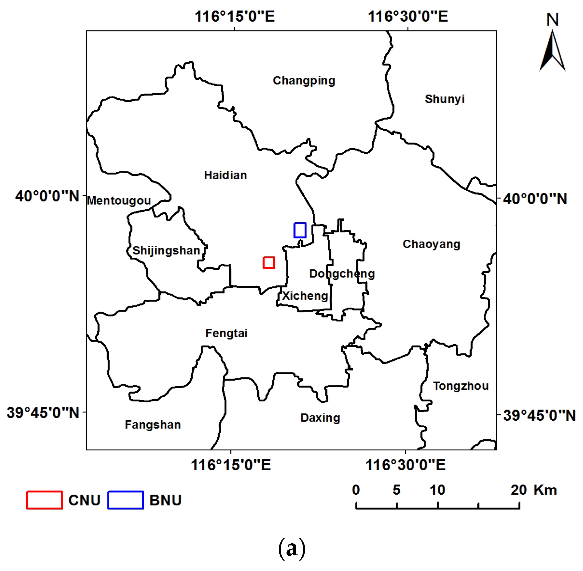
In this study, we aimed to evaluate bi-temporal high spatial resolution imagery for tree species classification in a more complex urban environment, exemplified by two study areas in Beijing, China which represent typical tree distribution in big cities. Unlike the study area in Berlin, urban tree coverage in inner-city Beijing makes up only 25.2% [
15]. Trees are mainly isolated and distributed along roadsides, as well as around residential areas, school campuses, or within parks; trees are either individually distributed or clustered in groups of several trees. Tree crown sizes vary and the crown diameter is normally within 3–8 meters. In these cases, the spatial resolution of RapidEye imagery is likely too coarse to identify crown spectral and texture characteristics. Higher spatial resolution imagery needs to be utilized to conduct tree classification at the species level. Moreover, a pixel-based classification method such as that used for RapidEye imagery cannot be used for species classification. In this study, we examined higher spatial resolution imagery,
i.e., WV2 and WV3 images, for bi-temporal analysis with an object-based method. At each of the two study sites, three classification schemes, including classification based on late summer WV2 images, high autumn WV3 images and both WV2 and WV3 images, were conducted to examine the effects of bi-temporal imagery on urban tree species classification. Two machine learning algorithms, SVM and Random Forest (RF) were used for object-based classification. Comparisons between the two study sites were also performed in order to analyze the impact of a complex urban environment on tree species discrimination.
3. Methods
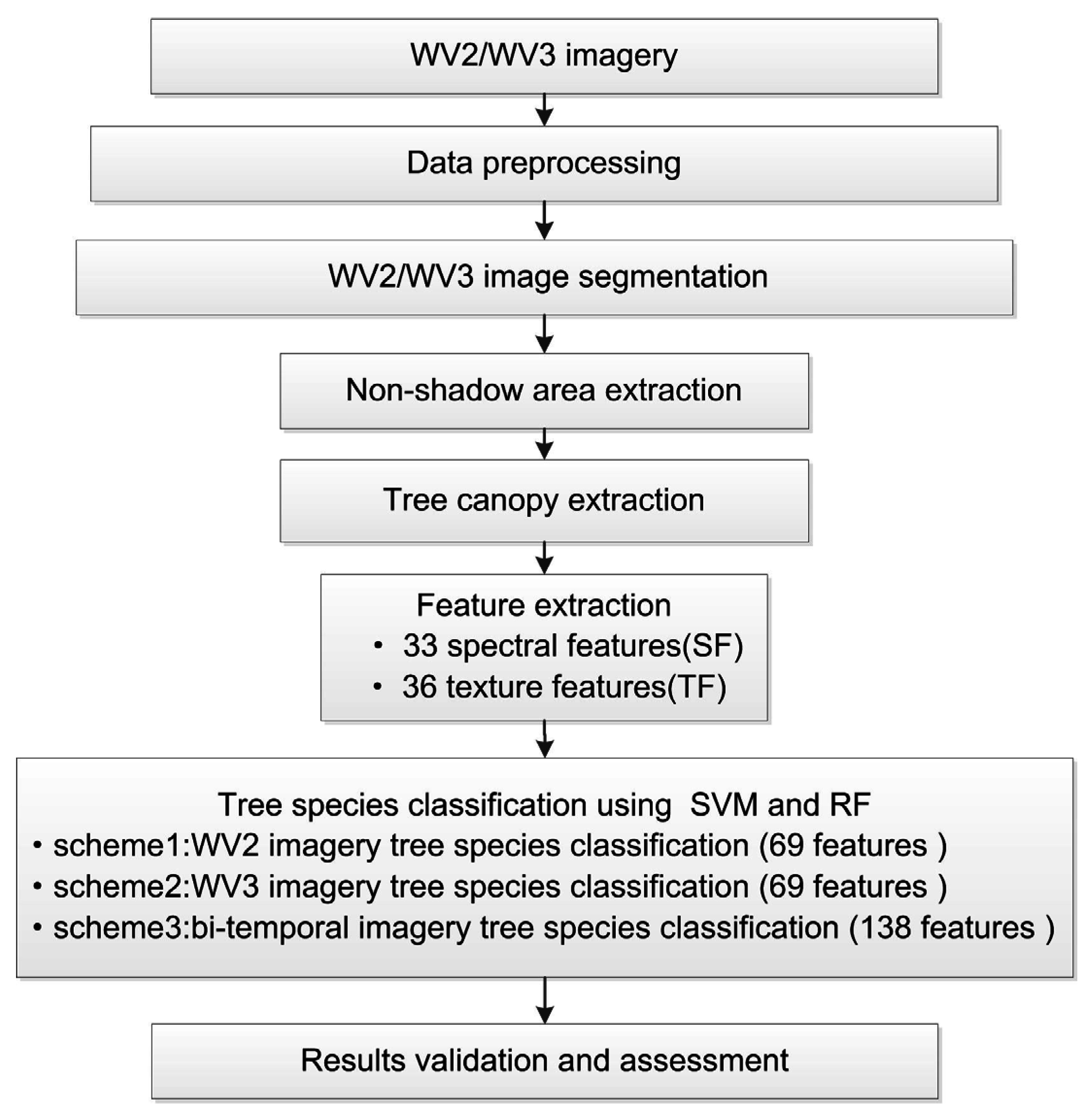
Figure 3 presents the flowchart of the urban tree species classification procedure using an object-based method and machine learning algorithms. The procedure consists of five steps: (1) data preprocessing; (2) images’ object generation by image segmentation; (3) tree crown area extraction; (4) feature extraction; and (5) tree species classification using machine learning algorithms SVM and RF. In order to evaluate the effect of bi-temporal images on urban tree species identification, for each study site three classification schemes were tested: classification based solely on the WV2 image, WV3 image, and a combination of WV2 and WV3 images. Accuracy assessment was then performed for each classification scheme. A tree species classification map was finally produced based on the best results.
Figure 3.
Flowchart of the tree species classification procedure.
Figure 3.
Flowchart of the tree species classification procedure.
3.1. Data Preprocessing
Each of the WV2 and WV3 panchromatic and multispectral Digital Number (DN) images was converted to Top of Atmosphere (TOA) radiance based on radiometric calibration parameters [
20] and standard correction formula [
21]. For each band, surface reflectance was generated using Second Simulation of a Satellite Signal in the Solar Spectrum Vector (6SV) [
22] radiative transfer algorithm based on a sensor spectral response function and specified atmospheric condition. A mid-latitude summer climate model was used to specify water vapor and ozone content. Aerosol optical thickness was obtained from MODIS Aerosol product (MOD04_L2) on the same day. Then the 2 m multispectral WV2 (or WV3) surface reflectance image was fused with 0.5 m panchromatic WV2 (or WV3) surface reflectance image to generate a pan-sharpened 0.5 m WV2 (or WV3) image using the Gramm-Schmidt Spectral Sharpening (GSPS) method with nearest-neighbor resampling [
23]. Studies have proven that this pan-sharpening method could reflect the synergic effectiveness of both multispectral and high resolution panchromatic images. It has also proved that this method is spectrally stronger than other sharpening techniques for the fusion of WV2 multispectral bands with the panchromatic band [
24]. The GSPS method has been widely applied in land cover classification [
25], forest tree species classification [
26], urban tree species classification [
12], and detection of mineral alteration in a marly limestone formation [
27]. In our study, the pan-sharpened image provides clear boundaries of tree crowns, and thus was used for further processing including segmentation and classification.
Both WV2 and WV3 pan-sharpened images were co-registered to eliminate small location displacement of tree crowns caused by differences in image acquisition time and satellite observation angle. The co-registration error, i.e., Root Mean Square Error, was within 0.5 pixel size (0.28 pixel at BNU study area and 0.17 pixel at CNU study area).
3.2. Image Segmentation
Multi-resolution segmentation algorithm in Trimble eCognition
TM Developer 8.7 software was used to generate image objects from each of the pan-sharpened WV2 and WV3 images. The multi-resolution segmentation algorithm is a bottom-up region merging technique. Starting from one-pixel objects, larger objects are generated by merging smaller ones with a series of iterative steps [
28]. Parameters required as input for the segmentation algorithm include: (1) weight of each input layer; (2) scale parameter; (3) color/shape weight; and (4) compactness/smoothness weight. In this study, all of the eight spectral bands of WV2 or WV3 pan-sharpened imagery were used as input. Previous research has shown that the eight WV2 bands are equally important for urban land cover classification [
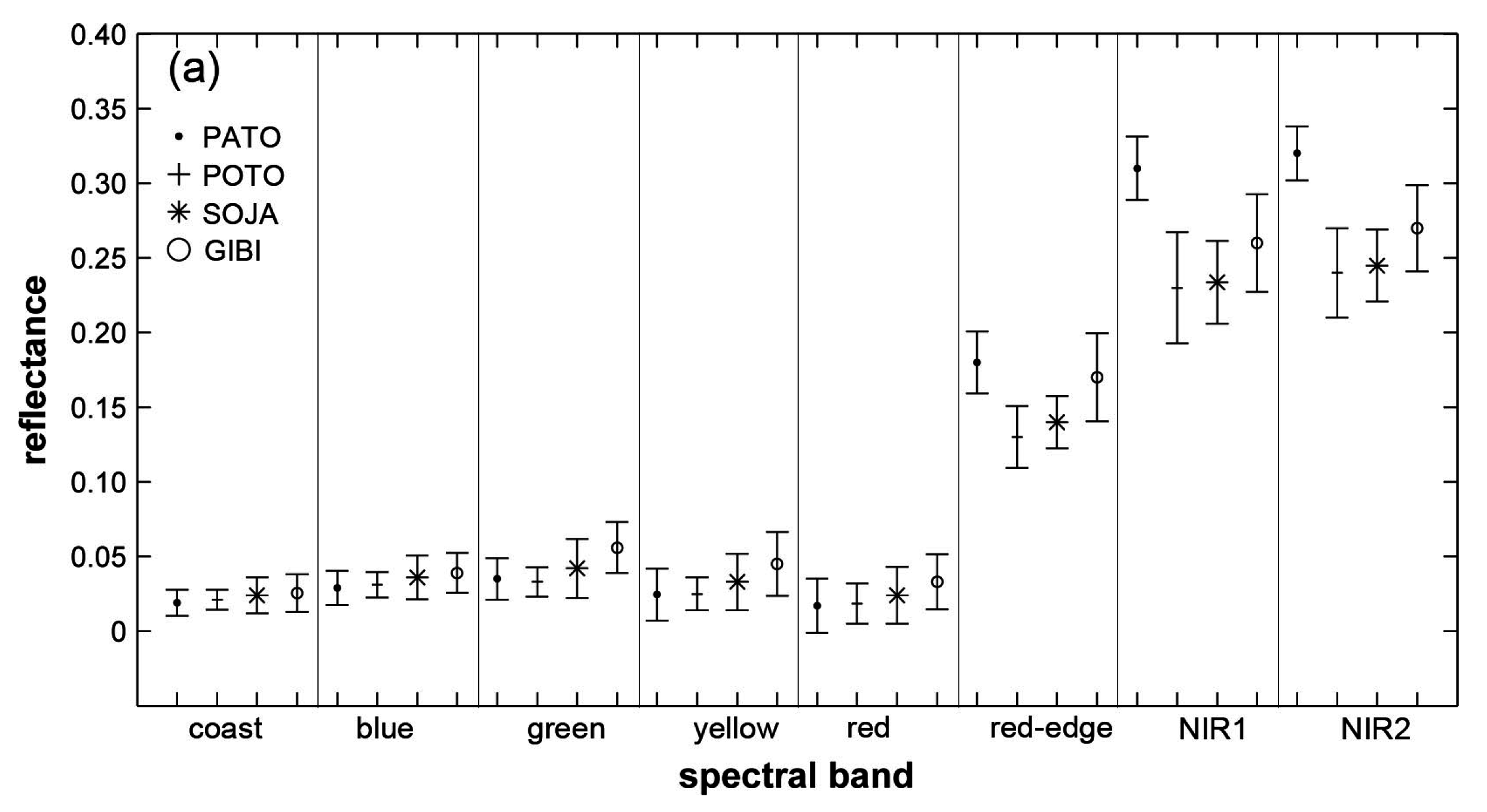
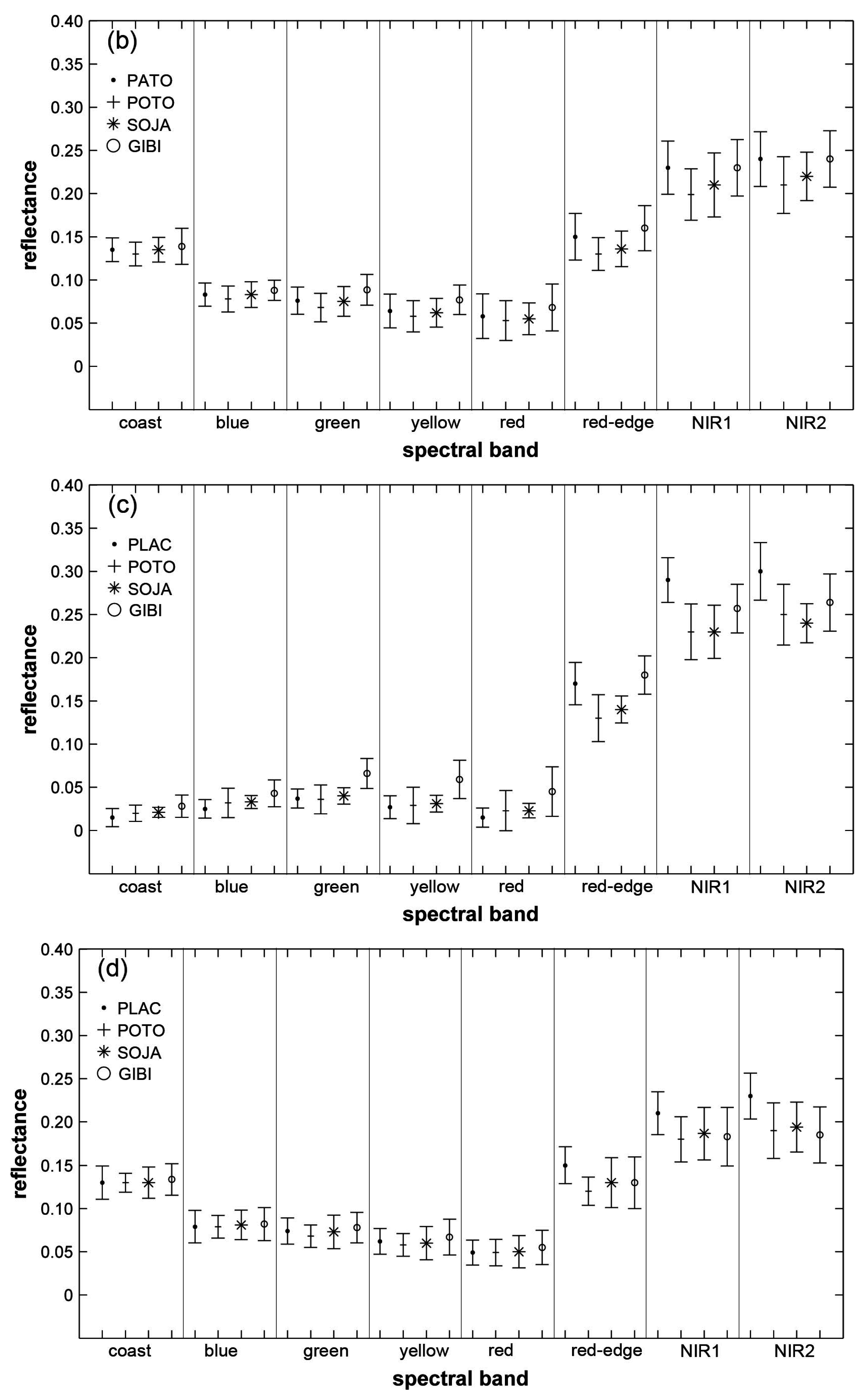
29]. Furthermore, as is shown in
Figure 2, the spectral reflectance of the species are different at each of the eight bands, and it is hard to tell which bands are more important in distinguishing these species. Therefore, all of the eight spectral band layers were assigned the same weight in the segmentation process. The weights of color and compactness were set as 0.8 and 0.5, respectively, in order to balance the difference of spectral/shape heterogeneity between tree species and buildings. For bi-temporal classification, segmented polygons from each of the single-date images were intersected to generate new image objects.
For object-based classification, scale parameter is a key factor because it is closely related to the resultant image object size [
30,
31]. Under- or over-segmentation both decreases classification accuracy, although significant under-segmentation tends to produce much worse results than over-segmentation [
9,
32,
33]. In this study, we adopted the Bhattacharyya Distance (BD) index method presented by Xun
et al. [
25] and Wang
et al. [
26] in order to determine the best segmentation scale parameter. In statistics, BD is used to measure the similarity between two discrete or continuous probability distributions and the amount of overlap between two statistical samples. In remote sensing, a greater BD value corresponds to greater spectral separation between two distinct classes. The BD index method assumed that the best scale parameter leads to the maximum separation of classes; thus, when the pair-wise BD values reach the highest, the corresponding scale parameter was selected as optimum. Six scale parameters, 100, 110, 120, 130, 140 and 150, were tested (
Table 3). For each segmented image, BD index values between every two tree species were calculated based on mean spectral reflectance of each band within the segmented polygons. The scale parameter that results in the overall maximum BD values was selected as optimal scale parameter. BD index equations are as follows:
where
i, j represent class
and class
,
is the Bhattacharyya Distance between tree species class
i and
j,
and
are the matrices composed of mean reflectance values of all polygons at each of the eight spectral bands.
and
are the covariance matrix of
and
, respectively;
is half of the sum of
and
. The result is a value in a range of 0 to 2, with greater BD values representing greater separability.
Table 3.
Parameters for pan-sharpened WV2/WV3 image segmentation.
Table 3.
Parameters for pan-sharpened WV2/WV3 image segmentation.
| Band Number | Input Layers | Weight | Scale Parameters | Color | Compactness |
|---|
| 1 | coastal | 1 | 100
110
120
130
140
150 | 0.8 | 0.5 |
| 2 | blue | 1 |
| 3 | green | 1 |
| 4 | yellow | 1 |
| 5 | red | 1 |
| 6 | red-edge | 1 |
| 7 | NIR1 | 1 |
| 8 | NIR2 | 1 |
3.3. Tree Canopy Extraction
Hierarchical classification strategy was utilized to extract tree crowns in non-shadow areas. Tree canopy under shadows casted by buildings were not considered in this study as it is difficult to recover accurate spectral information of tree crowns. First, shadow and non-shadow areas were separated with NIR1 threshold. Studies have demonstrated that urban land covers usually have higher reflectivity at the NIR spectrum than the visual spectrum, and the reflectance in the shadow area drops more significantly at the NIR band than the non-shadow area because of the occlusion of sunlight [
34]. The threshold value was determined using a bimodal histogram splitting method, which has been successfully used for shadow detection [
34,
35,
36]. Image objects with mean NIR1 reflectance values higher than the threshold were extracted as the non-shadow area. Next, vegetation was extracted from the non-shadow area with a NDVI threshold. Because there was an overlap between NDVI values of blue roofs (0.29–0.60 at CNU and 0.22–0.64 at BNU) and those of vegetation (0.35–0.98 at CNU and 0.43–0.99 at BNU), we further used the blue band threshold to remove these buildings because blue roofs have significantly higher blue band reflectance than vegetation. Both NDVI and blue band thresholds were determined with a stepwise approximation method [
12], which searches an initial threshold values in the histogram and then identifies the optimal threshold value as the one that results in the best match with reference polygons. Finally, tree canopy objects were separated from the other vegetated areas such as grass and shrub. New metrics were first calculated by multiplication of a textural feature such as Grey Level Co-occurrence Matrix Entropy (GLCME) of NIR1 band (GLCME
NIR1) or Grey Level Difference Vector Angular Second Moment (GLDVA) of NIR1 band (GLDVA
NIR1) and a color feature such as hue or intensity. Both texture and color features were considered because of the observations that tree canopy normally had a higher GLCME
NIR1 value or hue values than grass/shrub, and lower GLDVA
NIR1 or intensity values. All combinations of GLCME
NIR1, GLDVA
NIR1, hue and intensity values were evaluated. Similar as the vegetation/non-vegetation classification, threshold values were determined using the stepwise approximation method. After trial and error, threshold values of GLCME
NIR1 × hue metrics and GLDVA
NIR1 × intensity metrics were chosen for the CNU and BNU areas, respectively (
Table 4). The accuracy of tree crown extraction was approximately 95% for both sites.
Table 4 summarized all threshold values for each classification step.
Table 4.
Threshold values for hierarchical classification steps.
Table 4.
Threshold values for hierarchical classification steps.
| | Non-Shaded Area | Vegetation | Tree Canopy |
|---|
| CNU_WV2 | NIR1 ≥ 0.083 | NDVI > 0.35 and blue < 0.075 | GLCMENIR1 × hue > 2.45 |
| CNU_WV3 | NIR1 ≥ 0.094 | NDVI > 0.35 and blue < 0.12 | GLCMENIR1 × hue > 2.6 |
| BNU_WV2 | NIR1 ≥ 0.063 | NDVI > 0.43 and blue < 0.077 | GLDVANIR1 × intensity < 0.0019 |
| BNU_WV3 | NIR1 ≥ 0.085 | NDVI > 0.33 and blue < 0.12 | GLDVANIR1 × intensity < 0.0013 |
3.4. Tree Canopy Feature Extraction
For tree canopy objects on each of the WV2 and WV3 images, a total of 69 features including 33 spectral features and 36 textural features were extracted from the pan-sharpened eight-band image in addition to the first principal component layer derived by Principal Component Analysis (PCA). As listed in
Table 5, spectral features consisted of means and standard deviations of surface reflectance of each band, ratios calculated by mean spectral value of each band divided by the sum of spectral values of all eight bands, NDVIs derived from red, NIR1 bands and four additional bands, brightness values derived from the traditional bands (band 2, 3, 5, 7) and additional bands (band 1, 4, 6, 8), and mean and standard deviation of the first principal component image. Textural features included 24 GLCM and 12 GLDV features [
9,
37]. GLCM is a tabulation of the frequency of different combinations of grey levels at a specified distance and orientation in an image object, and GLDV is the sum of the diagonals of the GLCM within the image object [
9,
28]. The spectral indices were considered because they reflect spectral discrimination between tree species. Texture indices were used because tree crowns with different species have different crown structures and distribution of branches or twigs. All these spectral and textural indices are potentially useful for forest or urban tree species classification [
9,
12]. The first principle component image accounts for most of the variance in the eight bands. Previous research [
38] has shown that PCA analysis helped discrimination of trees, grass, water and impervious surfaces in urban areas. The 69 features were used for each single-date classification scheme. For the bi-temporal classification scheme, a total of 138 features, including 69 features from each of the WV2 and WV3 images, were used. Note that object geometric features such as size, shape index, or length/width ratio were not incorporated because an image segment may consist of several connected trees, and could therefore not represent shape and size characteristics of each tree crown.
Table 5.
Description of object features derived from WV2/WV3 images.
Table 5.
Description of object features derived from WV2/WV3 images.
| Feature Name | Description |
|---|
| Mean1-8 | Mean of bands 1–8 |
| SD1-8 | Standard deviations of individual bands 1–8 |
| Ratio1-8 | ith band mean divided by sum of band 1 through band 8 means |
| BTRA | Brightness derived from traditional bands 2, 3, 5, 7 |
| BADD | Brightness derived from additional bands 1, 4, 6, 8 |
| NDVI75 | (band7 − band5)/(band7 + band5) |
| NDVI86 | (band8 − band6)/(band8 + band6) |
| NDVI84 | (band8 − band4)/(band8 + band4) |
| NDVI61 | (band6 − band1)/(band6 + band1) |
| NDVI65 | (band6 − band5)/(band6 + band5) |
| GLCMH | GLCM homogeneity from bands 3, 6, 7, 8 |
| GLCMCON | GLCM contrast from bands 3, 6, 7, 8 |
| GLCMD | GLCM dissimilarity from bands 6, 7, 8 |
| GLCMM | GLCM mean from bands 3, 6 |
| GLCME | GLCM entropy from bands 3, 6, 7, 8 |
| GLCMSD | GLCM standard deviation from bands 3, 6, 7, 8 |
| GLCMCOR | GLCM correlation from bands 6, 7, 8 |
| GLDVA | GLDV angular second moment from bands 6, 7, 8 |
| GLDVE | GLDV entropy from bands 6, 7, 8 |
| GLDVC | GLDV contrast from bands 3, 6, 7, 8 |
| GLDVM | GLDV mean from bands 3, 6 |
| PCAM | Mean of the first principal component from Principal Component Analysis |
| PCASD | Standard deviation of first component from Principal Component Analysis |
3.5. Tree Species Classification
Image objects that intersected with reference polygons were used as reference samples. The number of samples for each tree species was summarized in
Table 6. For each classification scheme at each study area, two machine learning algorithms, Support Vector Machine (SVM) and Random Forest (RF), were used to mode the classifiers.
Table 6.
Number of sample objects for each study area.
Table 6.
Number of sample objects for each study area.
| Study Area | Tree Species | WV2 | WV3 | Bi-Temporal |
|---|
| CNU | PATO | 98 | 98 | 260 |
| POTO | 269 | 214 | 620 |
| SOJA | 205 | 157 | 396 |
| GIBI | 74 | 50 | 87 |
| Sum | 646 | 519 | 1363 |
| BNU | PLAC | 168 | 115 | 397 |
| POTO | 448 | 303 | 726 |
| SOJA | 459 | 335 | 814 |
| GIBI | 241 | 187 | 259 |
| Sum | 1316 | 940 | 2196 |
Support Vector Machine (SVM) was developed by Cortes and Vapnik [
39]. It attempts to find the optimal hyper plane in the high-dimensional feature space to maximize the margin between classes with a kernel function in polynomial, radial basis, or sigmoid form. SVM has proved to perform well in handling small numbers of training samples with high-dimensional space [
14,
40,
41]. In this study, we used Radial Basis Function Kernel (RBF) as the kernel function because it works well in many classification tasks [
42,
43,
44]. Optimal classifier parameters including RBF kernel parameter
and penalty factor
were determined by the grid search method in the LibSVM software package [
45].
Random Forest (RF) [
46] is constituted by many Classification and Regression Trees (CARTs) and suitable for high-dimensional dataset classification [
40,
47,
48]. Each decision tree in RF is constructed by extracting an individual bootstrap sample (sampling with replacement) from the original dataset. The splitting variables used at each node are determined based on the Gini Index [
7,
40,
49,
50,
51]. Then, each tree assigns the single vote to the most frequent class for the input data. To finish, the class gaining the majority vote is classified into the corresponding category. RF employed out-of-bag (OOB) samples that are not in the bootstrap samples to estimate the prediction performance. During classification, two important parameters [
7,
49] are necessary: (1) ntree,
i.e., the number of decision trees executing classification; and (2) mtry,
i.e., the number of input variables used at each node. In this study, we tried the parameter ntree ranging from 100 to 1000 and mtry as 1, 8 or 11 (the square root of the number of features) to determine the best group setting. After trial and error, the validation results indicated that the accuracy reached its maximum with ntree = 500 and mtry = 8 for single-date image classification, and ntree = 500 and mtry = 11 for bi-temporal image classification. These parameters were thus used for RF classification in this study.
Image objects with over 10% of the area intersecting with the reference samples were used as sample objects. Ten-fold cross-validation with fixed subsets of training/validation sample objects was conducted to for each classifier and classification scheme. Each subset of the training/validation samples were selected based on a stratified random sampling process in order to ensure that the sample selected had a proportional number of each class. The average overall accuracy, kappa value, user and producer accuracy from validation datasets were used to assess the classification performance.
4. Results
4.1. Selection of Optimal Image Segmentation Scale Parameter
Pair-wise BD values were calculated for each image at each study area.
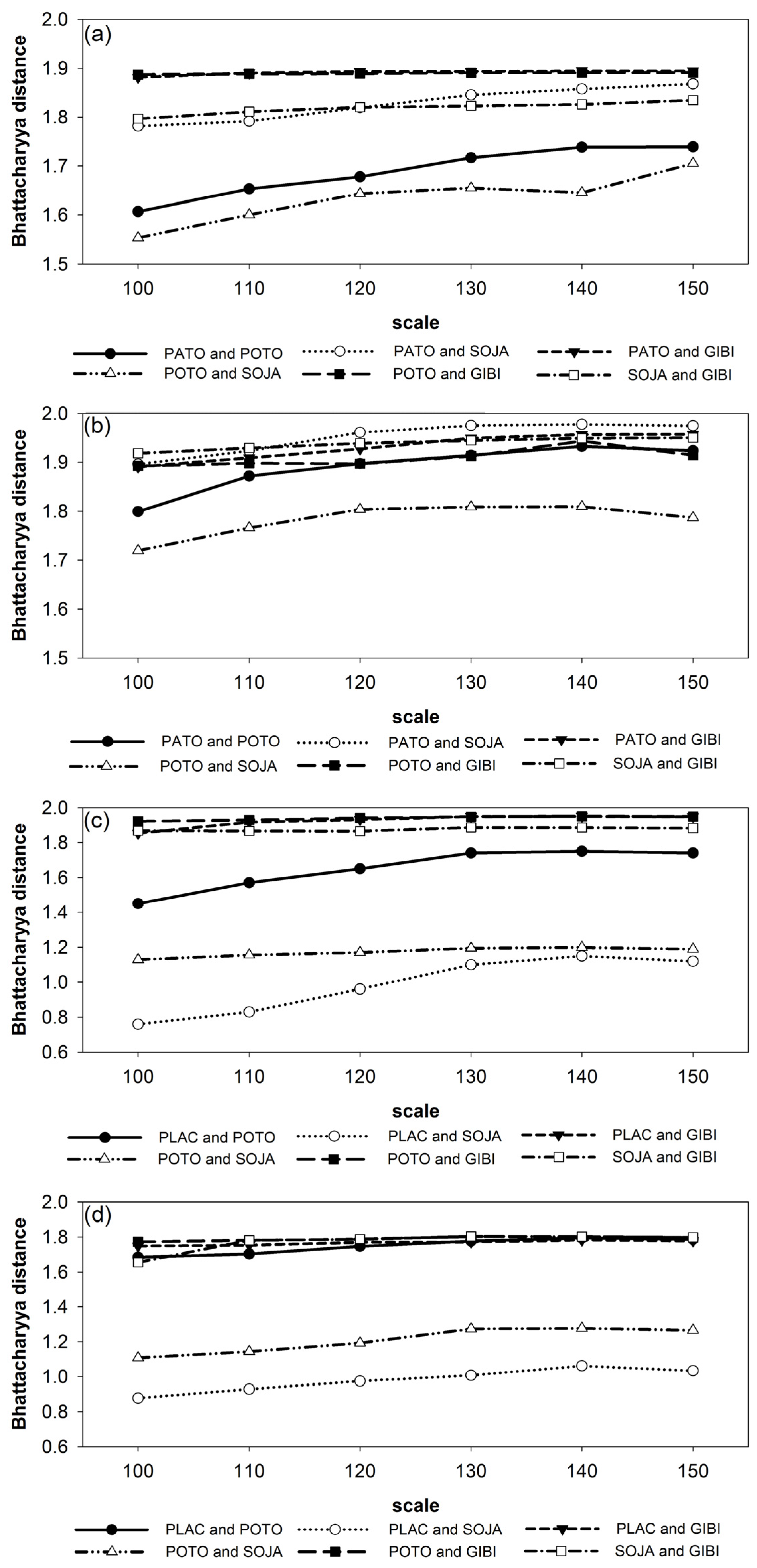
Figure 4 shows that at both areas, BD values of all six pairs of species increase gradually with a scale parameter ranging from 100 to 130. For the WV2 image at CNU (
Figure 4a), all BD values except that between POTO and SOJA reach their maximum at the scale parameter of 140 and become stable from 140 to 150. The maximum BD between POTO and SOJA is obtained at a scale parameter of 150. Thus, 150 was selected as the best scale parameter. For the WV3 image at CNU, all BD values reach a plateau at a scale parameter of 140, thus 140 was selected as best scale parameter (
Figure 4b). Similarly, 140 was selected as best scale parameters for both images at BNU (
Figure 4c,d). In both study areas, the number of tree stems per segment varies from one to eight depending on the tree crown layout. For individual tree crowns, each segment only covers one tree crown. For connected tree crowns (for example, Chinese white poplars on the CNU campus are planted densely along the avenue), one segment may cover as many as eight stems.
At both study sites, GIBI and any other species always have higher BD values, thereby indicating that GIBI has better spectral separability from other species, and thus better classification accuracy is expected. POTO and SOJA species always have smaller BD values, meaning that the two species are less spectrally separable. PLAC and SOJA, PATO and POTO species are also less separable. Overall, BD values at BNU are lower than those at CNU; lower overall classification accuracy is therefore expected.
Figure 4.
BD values between six pairs of tree species at image segmentation scales from 100 to 150. (a) BD values from WV2 image at CNU; (b) BD values from WV3 image at CNU; (c) BD values from WV2 image at BNU; (d) BD values from WV3 image at BNU.
Figure 4.
BD values between six pairs of tree species at image segmentation scales from 100 to 150. (a) BD values from WV2 image at CNU; (b) BD values from WV3 image at CNU; (c) BD values from WV2 image at BNU; (d) BD values from WV3 image at BNU.
4.2. Classification Results
Table 7 lists the average overall accuracy (OA) and kappa values from all classification schemes at both study sites. The OAs range from 70.0% to 92.4% at the CNU study site, and from 71.0% to 83.0% at the BNU study site. Using either the SVM or RF algorithm, tree species classification based on bi-temporal WV2 and WV3 images produces considerably higher accuracies than those based on each image alone at both study sites, with an average increase in OA of 11.5%. At CNU, the OA is around 9.7%–20.2% higher than when using a single-date image, regardless of the classification method used. Kappa values based on bi-temporal images are higher than 0.85, while those based on single-date images can be as low as 0.56. At BNU, OAs from bi-temporal image classification increase around 5%–12% compared to single-date image classification, and kappa values increase from less than 0.60 to over 0.75.
Table 7.
Classification results with single-date images and bi-temporal images using the SVM and RF methods in the CNU and BNU areas. OA: overall accuracy.
Table 7.
Classification results with single-date images and bi-temporal images using the SVM and RF methods in the CNU and BNU areas. OA: overall accuracy.
| Classification Schemes | CNU | BNU |
|---|
| SVM | RF | SVM | RF |
|---|
| OA(%) | Kappa | OA(%) | Kappa | OA(%) | Kappa | OA(%) | Kappa |
|---|
| WV2 | 82.7 | 0.75 | 77.2 | 0.67 | 75.6 | 0.66 | 71.0 | 0.59 |
| WV3 | 76.3 | 0.66 | 70.0 | 0.56 | 74.2 | 0.64 | 72.7 | 0.62 |
| bi-temporal | 92.4 | 0.89 | 90.2 | 0.85 | 80.3 | 0.76 | 83.0 | 0.76 |
Radar charts in
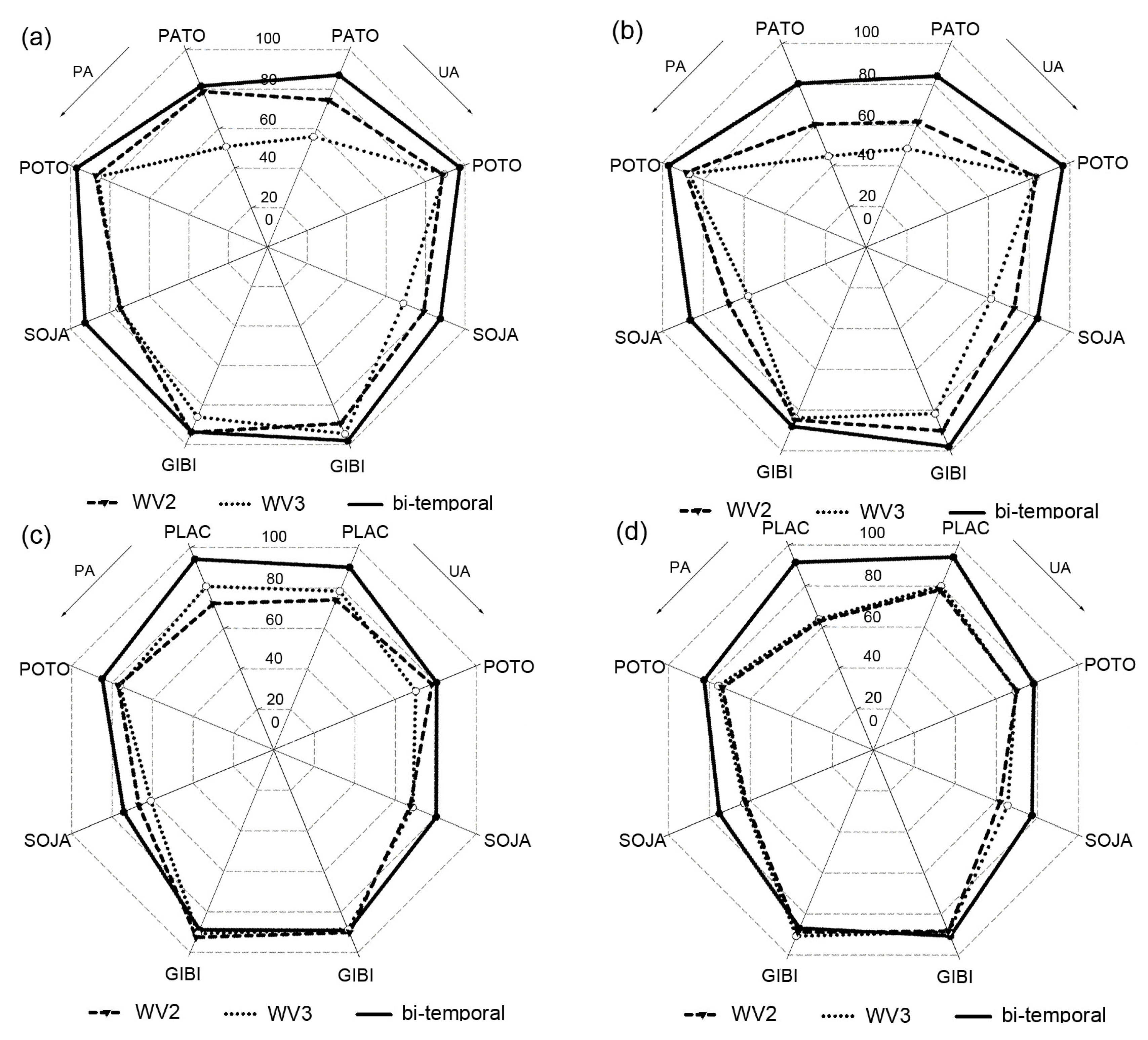
Figure 5 show that for almost all tree species, both producer accuracies (PAs) and user accuracies (UAs) derived from bi-temporal image classification are notably higher than those from single-date image classification; the increases of PAs and UAs are on average 10.7%. At CNU, PAs of SOJA species increase by over 15% regardless of classification algorithm used, and UAs increase by over 11%; PATO has low PA and UA (44.7%–56.0%) based on the WV3 image alone, which may be caused by the small spectral reflectance gap between PATO and other species during high autumn (
Figure 2b), while the addition of the WV2 image acquired in late summer helps increase the accuracy to 81.5%–87.1%. At BNU, PA of PLAC increase from 62.9% to 91.2% and UA increase from 78.2% to 94.2%. GIBI has relatively higher PAs and UAs than other species at both study sites using either WV2 or WV3 images. Especially at BNU, both PA and UA of GIBI are over 85%, while PA and UA of other species are lower than 80%. PATO, PLAC and SOJA had lower PA and UA when single-date images were used in the classification in each area. However, when using a combination of WV2 and WV3 images, PA and UA of PATO and SOJA at CNU, and PLAC at BNU increase substantially and are comparable with those of GIBI species (
Figure 5). It is evident that bi-temporal classification not only produces higher but also more balanced PAs and UAs among tree species. The standard deviation of PAs of all species decreases from 11.7% using a single-date image to 6.2% using a bi-temporal image, and that of UAs decreases from 13.6% to 6.4%.
Table 7 demonstrates that OAs at the CNU site are consistently higher than those from BNU, regardless of the classification methods or schemes. For example, the overall accuracy generated from WV2 images using the SVM classifier at CNU is about 7% higher than that at BNU. For the same dominant species at both sites,
i.e., POTO, SOJA and GIBI, both PAs and UAs at CNU are higher than those at BNU (
Figure 5). Comparisons between SVM and RF classification results show that SVM is superior to RF at both sites (
Table 7 and
Figure 5). OAs from SVM were around 1.5%–6.3% higher than those from RF except that from the bi-temporal classification scheme at BNU. TheSVM classifier was thus used for tree species mapping.
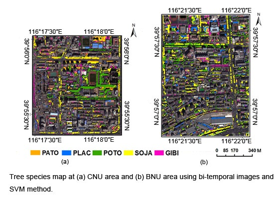
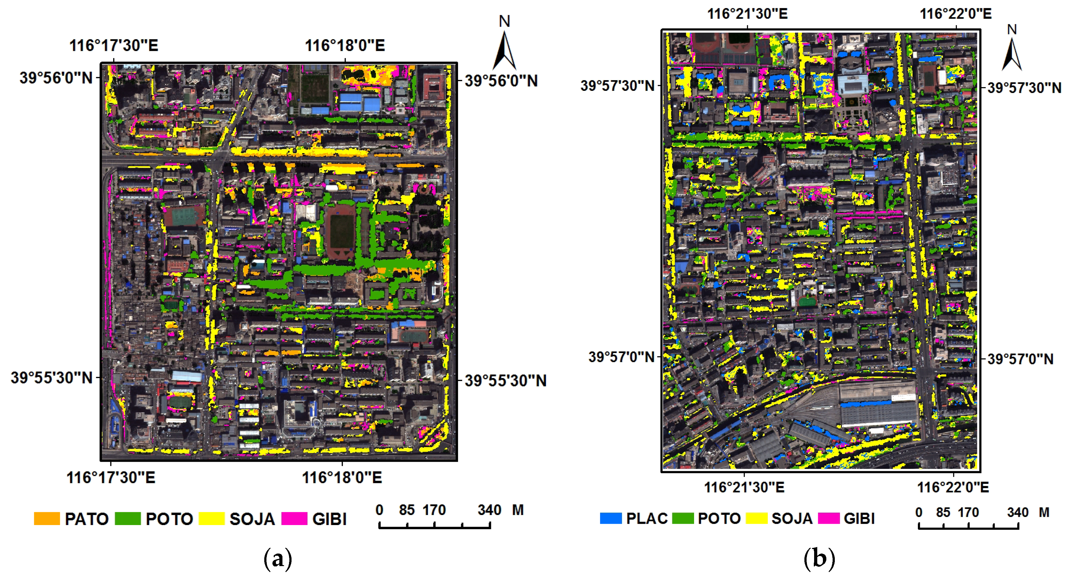
Figure 6 illustrates the resultant classification maps for dominant tree species using the SVM method based on bi-temporal images over both areas. Minor tree species were classified as one of the dominant classes. It is obvious that the classification map at BNU is more fragmented than that at CNU.
Figure 5.
Radar charts of three classification schemes with SVM and RF methods in two study areas. (a) PAs and UAs using SVM at CNU; (b) PAs and UAs using RF at CNU; (c) PAs and UAs using SVM at BNU; (d) PAs and UAs using RF at BNU. PA: producer accuracy; UA: user accuracy.
Figure 5.
Radar charts of three classification schemes with SVM and RF methods in two study areas. (a) PAs and UAs using SVM at CNU; (b) PAs and UAs using RF at CNU; (c) PAs and UAs using SVM at BNU; (d) PAs and UAs using RF at BNU. PA: producer accuracy; UA: user accuracy.
Figure 6.
Tree species map at (a) CNU area and (b) BNU area using bi-temporal images and SVM method.
Figure 6.
Tree species map at (a) CNU area and (b) BNU area using bi-temporal images and SVM method.
4.3. Feature Importance
Table 8 and
Table 9 list the first 20 important metrics ranked by SVM and RF classifiers in the bi-temporal classification scheme. F-score and Mean Decrease Accuracy (MDA) were used to calculate feature importance in SVM and RF, respectively. F-score is a tool embedded in LibSVM software and measures the discrimination of two sets of real numbers [
52]. MDA is generally used to measure the contribution of each feature to prediction accuracy in the RF model and can be calculated by permuting the
mth features of each tree for the out-of-bag data [
53]. Higher F-score or MDA values indicate higher importance of the feature in classification.
Among the 138 features used for bi-temporal classification, the top 20 important features identified by the SVM and RF classifier are mostly dominated by spectral characteristics. In both the CNU and BNU areas, less than five textural features are listed in the top 20 features by either the SVM or RF classifier, indicating that the spectral features make a more significant contribution to the species classification than the textural features. In both study areas, both the F-score and MDA identify the red-edge band (Band 6), the new NIR band (NIR2, Band 8) and green band (Band 3) as the most important bands since the features based on these bands, such as WV2_NDVI86, WV3_SD6, WV2_Mean3 and WV3_Ratio6, are consistently listed among the top-ranking features. Compared to the traditional four bands of high resolution satellite sensors, the new bands, especiallythe red-edge and NIR2 band designed for WV2 and WV3, make more of a contribution to urban tree species identification. In the two study areas, both WV2 and WV3 features are listed as important. Removing features derived from either WV2 or WV3 result in a decrease in accuracy, thereby emphasizing the role of bi-temporal spectral information in urban tree species classification.
Table 8.
F-score weight of each feature in SVM for bi-temporal classification.
Table 8.
F-score weight of each feature in SVM for bi-temporal classification.
| Rank | CNU | Rank | BNU |
|---|
| Features | F-Score | Features | F-Score |
|---|
| 1 | WV2_Mean3 | 0.696 | 1 | WV2_Ratio6 | 0.479 |
| 2 | WV3_Mean3 | 0.511 | 2 | WV2_NDVI86 | 0.409 |
| 3 | WV2_Mean4 | 0.511 | 3 | WV3_Ratio6 | 0.403 |
| 4 | WV2_NDVI86 | 0.455 | 4 | WV2_Mean3 | 0.376 |
| 5 | WV3_SD6 | 0.446 | 5 | WV2_Mean4 | 0.331 |
| 6 | WV3_SD3 | 0.353 | 6 | WV3_SD6 | 0.309 |
| 7 | WV3_SD5 | 0.344 | 7 | WV2_Mean6 | 0.288 |
| 8 | WV3_PCASD | 0.343 | 8 | WV2_SD6 | 0.249 |
| 9 | WV3_PCAM | 0.343 | 9 | WV2_Mean5 | 0.236 |
| 10 | WV3_Mean4 | 0.337 | 10 | WV3_Mean6 | 0.229 |
| 11 | WV3_SD2 | 0.322 | 11 | WV3_PCASD | 0.207 |
| 12 | WV3_SD4 | 0.322 | 12 | WV2_BADD | 0.196 |
| 13 | WV2_Ratio6 | 0.312 | 13 | WV2_PCASD | 0.189 |
| 14 | WV3_Ratio6 | 0.310 | 14 | WV2_BTRA | 0.187 |
| 15 | WV2_Mean5 | 0.304 | 15 | WV2_PCAM | 0.185 |
| 16 | WV2_Mean2 | 0.291 | 16 | WV3_NDVI61 | 0.185 |
| 17 | WV2_Mean1 | 0.262 | 17 | WV3_Mean3 | 0.184 |
| 18 | WV3_SD1 | 0.262 | 18 | WV2_GLDVE7 | 0.169 |
| 19 | WV3_SD8 | 0.261 | 19 | WV2_GLDVA8 | 0.167 |
| 20 | WV3_Mean2 | 0.254 | 20 | WV2_GLDVE8 | 0.165 |
Table 9.
MDA of each feature in RF for bi-temporal classification.
Table 9.
MDA of each feature in RF for bi-temporal classification.
| Rank | CNU | Rank | BNU |
|---|
| Features | MDA | Features | MDA |
|---|
| 1 | WV2_NDVI86 | 20.3 | 1 | WV2_Ratio6 | 24.7 |
| 2 | WV2_Ratio6 | 19.8 | 2 | WV2_NDVI86 | 20.0 |
| 3 | WV2_Mean3 | 16.1 | 3 | WV3_Ratio6 | 16.8 |
| 4 | WV3_SD6 | 15.1 | 4 | WV3_SD6 | 16.6 |
| 5 | WV3_PCASD | 13.6 | 5 | WV3_NDVI86 | 15.8 |
| 6 | WV3_Ratio6 | 13.5 | 6 | WV2_Mean3 | 15.7 |
| 7 | WV3_Mean5 | 13.3 | 7 | WV2_Ratio3 | 14. 4 |
| 8 | WV3_Mean3 | 13.2 | 8 | WV2_GLCMSD6 | 13.9 |
| 9 | WV3_SD8 | 12.7 | 9 | WV2_Ratio5 | 13.8 |
| 10 | WV3_NDVI86 | 12.6 | 10 | WV2_SD6 | 13.7 |
| 11 | WV2_GLCMM3 | 12.2 | 11 | WV3_Mean3 | 13.7 |
| 12 | WV2_Mean6 | 12.1 | 12 | WV2_NDVI65 | 13.6 |
| 13 | WV3_SD7 | 11.9 | 13 | WV3_NDVI65 | 13.2 |
| 14 | WV3_PCAM | 11.8 | 14 | WV3_GLCMM6 | 13.2 |
| 15 | WV2_SD6 | 11.7 | 15 | WV2_GLCMH8 | 13.0 |
| 16 | WV2_BTRA | 11.7 | 16 | WV2_GLDVA8 | 12.9 |
| 17 | WV2_Mean8 | 11.7 | 17 | WV3_Mean1 | 12.8 |
| 18 | WV2_GLDVC3 | 11.7 | 18 | WV3_SD7 | 12.7 |
| 19 | WV2_GLCMCON3 | 11.7 | 19 | WV2_NDVI57 | 12.6 |
| 20 | WV2_PCAM | 11.7 | 20 | WV3_GLDVA6 | 12.4 |
6. Conclusions
This study evaluated bi-temporal WV2 and WV3 imagery for tree species identification in complex urban environments. An object-based classification method based on SVM and RF machine learning algorithms was conducted using late summer WV2 images and/or high autumn WV3 images. Five dominant tree species, the empress tree (Paulownia tomentosa), Chinese white poplar (Populus tomentosa Carrière), Chinese scholar tree (Sophora Japonica), gingko (Ginkgo biloba) and London plane tree (Platanus acerifolia), were examined at two study sites in urban Beijing, China.
Results showed that phenology variations presented in the bi-temporal imagery helped enhance the species identification capability. The overall accuracies based on both WV2 and WV3 imagery reached 92.4% and were significantly higher than those based on single-date image alone. The PAs and UAs produced by a single-date image were relatively low (44.7%–82.5%) and could hardly satisfy requirements for most urban ecological assessment applications, whereas those derived from bi-temporal images were on average 10.7% higher, and the PAs and UAs more balanced. The feature importance analysis revealed that spectral characteristics were more important than texture features. The new wavebands designed for WV2 and WV3 sensors such as red-edge and NIR2 bands contributed more to the classification than the traditional four bands. Both WV2- and WV3-derived features are listed among the most important features. This highlights the necessity of bi-temporal or even multi-temporal high resolution images for urban tree species classification. Comparison between two study sites showed that urban environment heterogeneity and distribution pattern of trees in the study area influenced classification accuracy. Clustered and evenly distributed tree species were more easily identified than trees with scattered distribution. Our study also suggests that SVM is superior to RF in urban tree species classification as the former algorithm is more suitable for imbalanced sample distribution.
This study only identified the species in non-shadowed areas and did not consider the shadow effect on species classification. Our future research will focus on the development of approaches for spectral information restoration under shadowed areas in order to perform better and more complete tree species inventory. Because of the rounded shape of tree crowns, the uneven sun illumination within tree crowns may affect the species classification, especially for trees individually distributed. Impact of the uneven illumination on tree species classification will be incorporated in our future research. As the WV3 satellite could provide images in the 16-band mode, future research will also include evaluation of the eight shortwave infrared spectral bands in urban tree species classification.


