
Treating the Hooking Effect in Satellite Altimetry Data: A Case Study along the Mekong River and Its Tributaries


Abstract
:
1. Introduction

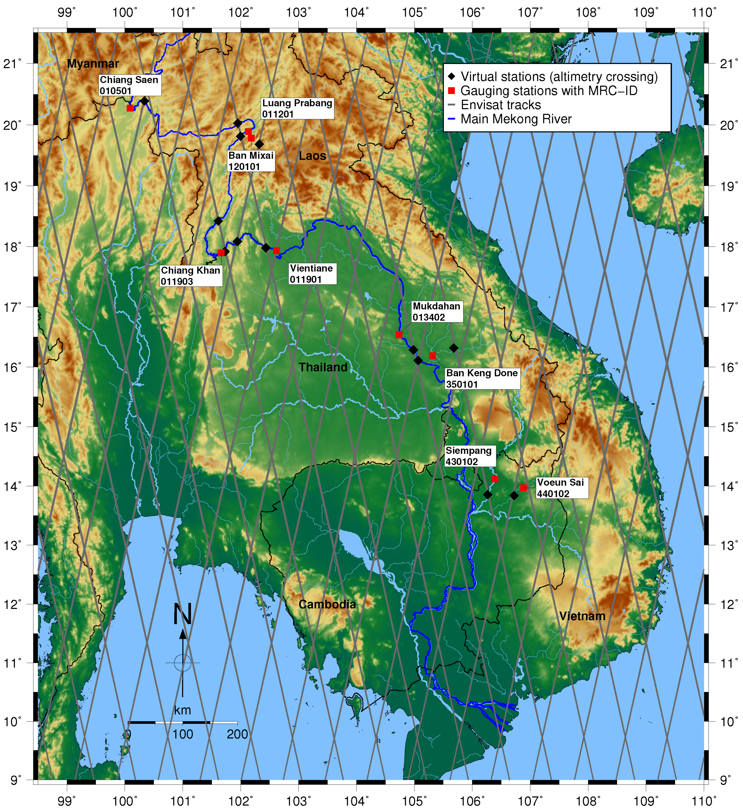
2. Study Area
3. Data
3.1. Altimetry Data

| Correction | Model/Source | Reference |
|---|---|---|
| ionosphere | NOAA Ionosphere Climatology 2009 (NIC09) | Scharroo and Smith [30] |
| dry troposphere | ECMWF (2.5°× 2.0°) for Vienna Mapping Functions 1 | Boehm et al. [31] |
| wet troposphere | ECMWF (2.5°× 2.0°) for Vienna Mapping Functions 1 | Boehm et al. [31] |
| polar tides | IERS Conventions 2003 | McCarthy and Petit [32] |
| earth tides | IERS Conventions 2003 | McCarthy and Petit [32] |
| geoid | EIGEN-6C3stat | Förste et al. [33] |
| oerr | MMXO14 | Bosch et al. [34] |
3.2. In-Situ Gauging Data

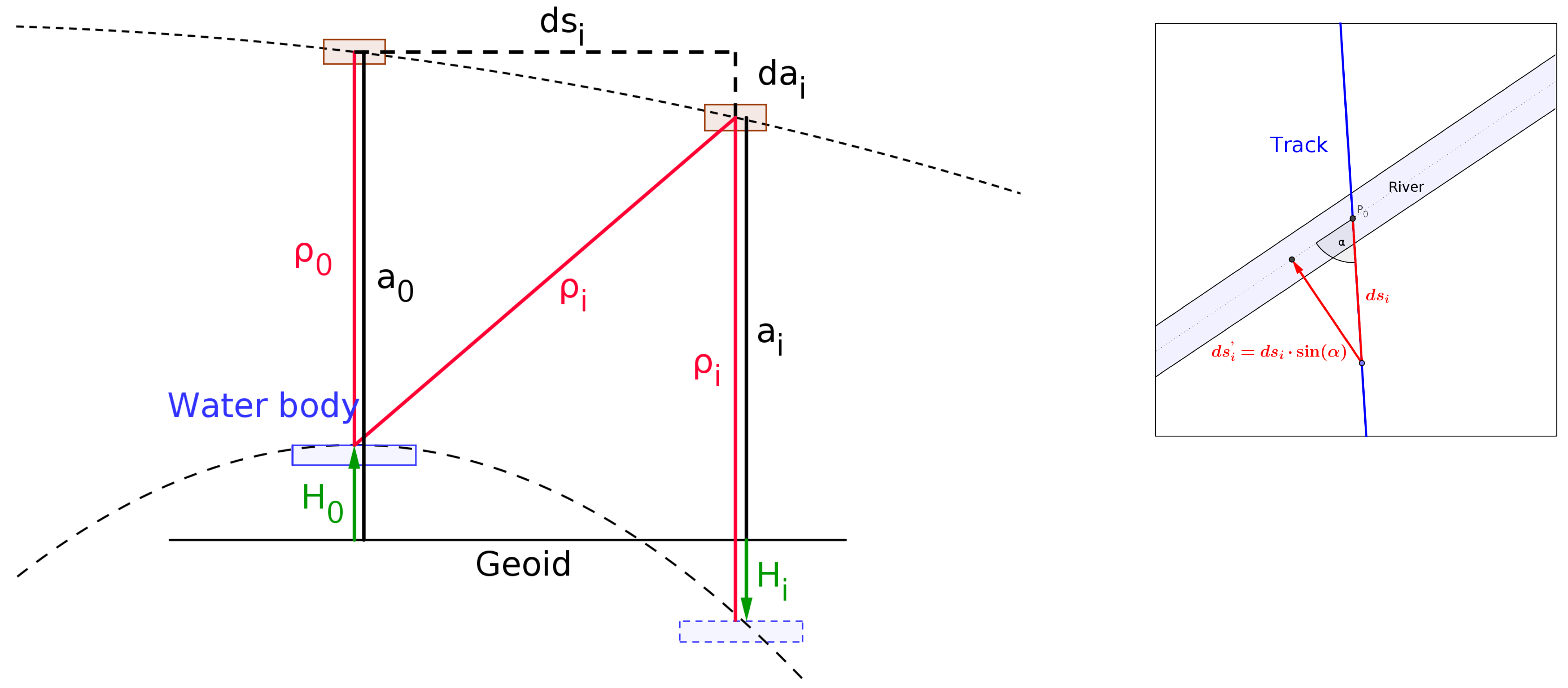
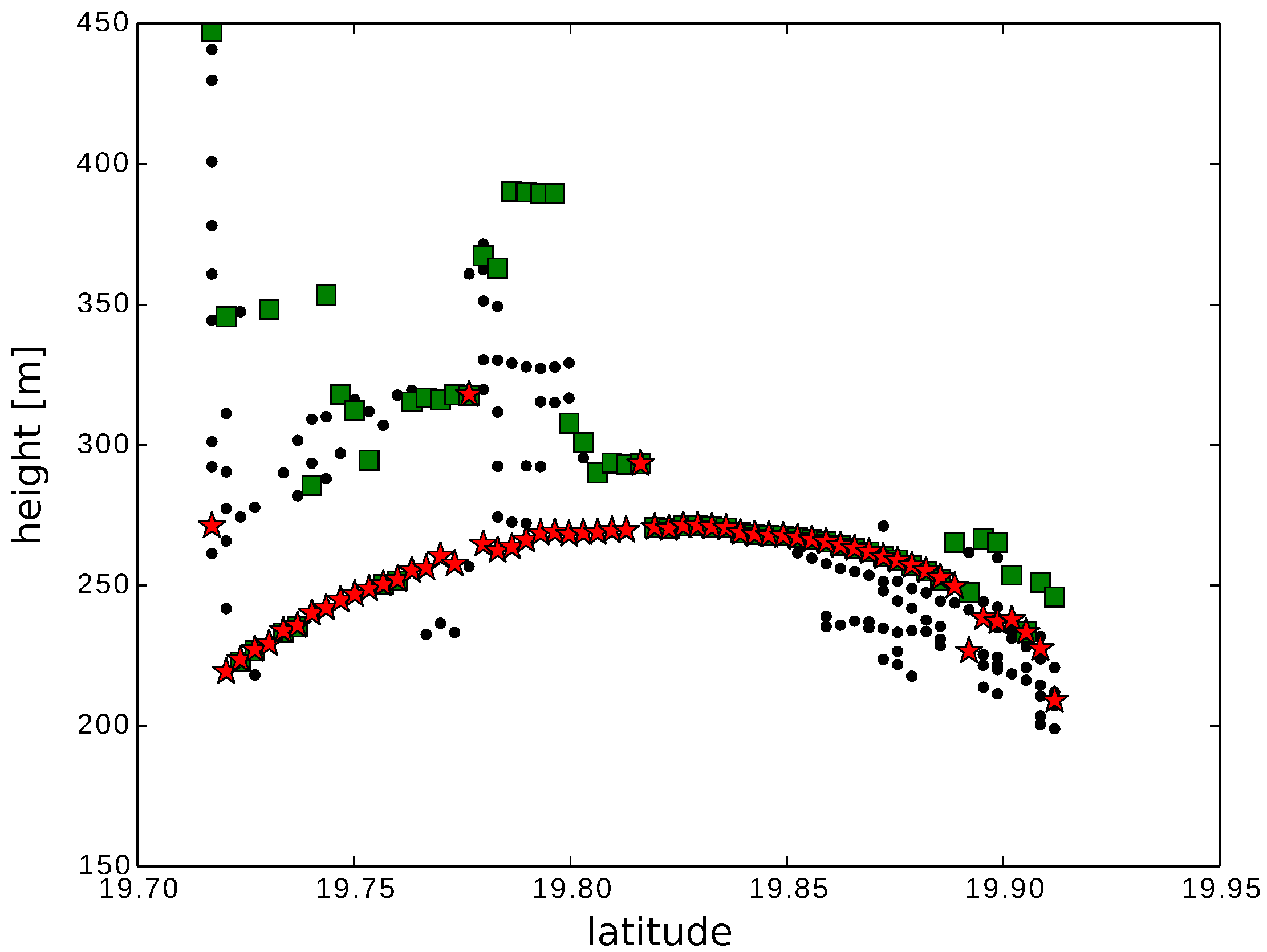
4. Hooking Effect

5. Method
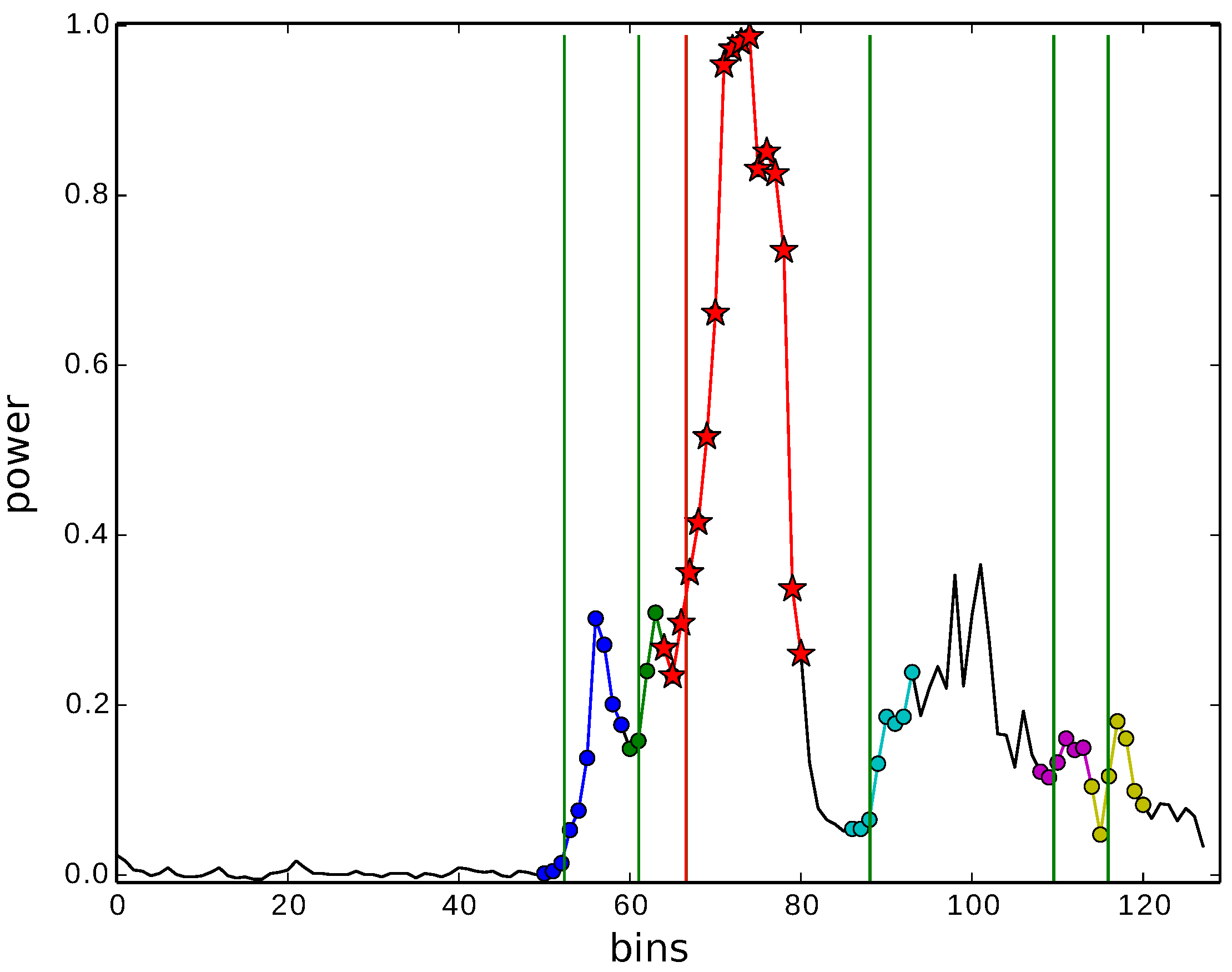
5.1. Multi-Subwaveform Retracker MSR


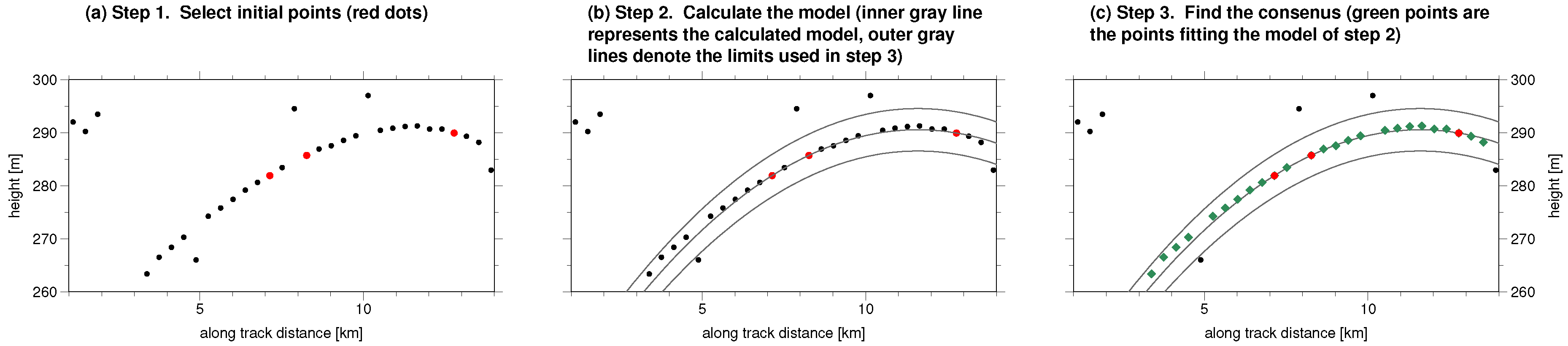
5.2. RANSAC Algorithm for Hooking Effect Estimation

- Select the initial values: A sufficient number of points to unambiguously define the model are randomly picked from all data points (e.g., 3 for a parabola and 2 for a line; see Figure 6a).
- Calculate the a-priori model: This step uses the randomly chosen points from step 1 (See Figure 6b).
- Find the consensus set:
- (a)
- The consensus set contains all data points that fit the model within a specified limit, which is determined by the accuracy of the points. Given the uncertainty in the data, if many data points fit the model the randomly picked starting points have probably homed-in on the correct model (See Figure 6c).
- (b)
- Recalculate the model using all points in the consensus set, and determine and save the new consensus set.
5.3. Final Parameter Estimation
5.4. Post-Processing of the Time Series
5.4.1. Slope Correction
5.4.2. Outlier Detection
6. Results, Validation and Discussion
6.1. Results and Validation of the Water-Level Time Series Derived by the Hooking Approach
| Hooking Approach | Median Approach | |||||||||||||||||
|---|---|---|---|---|---|---|---|---|---|---|---|---|---|---|---|---|---|---|
| without Outlier Detetction | with Outlier Detetction | |||||||||||||||||
| MCR Code | Station Name | Dist. | River Name | Pass | Lon | Lat | Intersect. Length | max. Amplitude | RMS | R2 | # Epochs | RMS | R2 | # Epochs | RMS | R2 | # Epochs | # Avail. Epochs |
| 010501 | Chiang Saen | 30 | Mekong River | 294 | 100.339 | 20.390 | 350 | 10 | 2.25 | 0.61 | 59 | 1.83 | 0.84 | 55 | 6.04 | 0.29 | 50 | 80 |
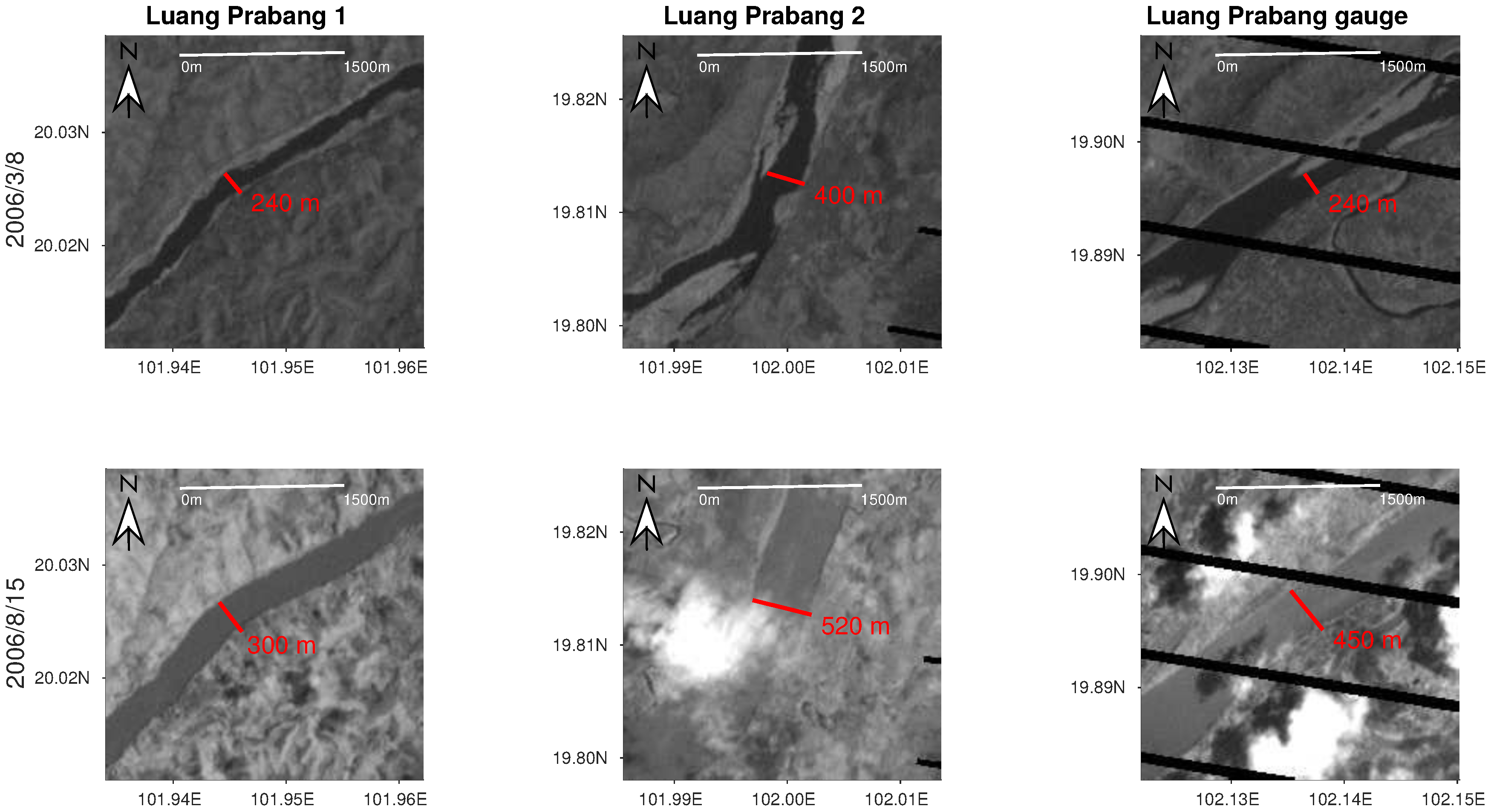
| 011201 | Luang Prabang 1 | 24 | Mekong River | 651 | 101.949 | 20.027 | 250 | 15 | 2.51 | 0.94 | 81 | 2.26 | 0.97 | 77 | 3.64 | 0.71 | 77 | 81 |
| Luang Prabang 2 | 16 | Mekong River | 651 | 102.000 | 19.814 | 500 | 15 | 1.23 | 0.88 | 76 | 1.20 | 0.91 | 73 | 6.96 | 0.26 | 76 | 79 | |
| 011903 | Chiang Khan 1 | 60 | Mekong River | 193 | 101.612 | 18.424 | 240 | 13 | 0.87 | 0.94 | 72 | 0.86 | 0.94 | 72 | 3.58 | 0.48 | 71 | 80 |
| Chiang Khan 2 | 5 | Mekong River | 193 | 101.730 | 17.919 | 2860 | 13 | 1.28 | 0.86 | 65 | 1.08 | 0.89 | 62 | 10.23 | 0.00 | 52 | 80 | |
| Chiang Khan 3 | 35 | Mekong River | 666 | 101.943 | 18.084 | 340 | 13 | 1.46 | 0.91 | 70 | 1.48 | 0.90 | 67 | 1.96 | 0.75 | 73 | 80 | |
| 011901 | Vientiane | 19 | Mekong River | 651 | 102.436 | 17.980 | 1800 | 11 | 1.63 | 0.76 | 71 | 1.22 | 0.86 | 69 | 6.30 | 0.03 | 82 | 82 |
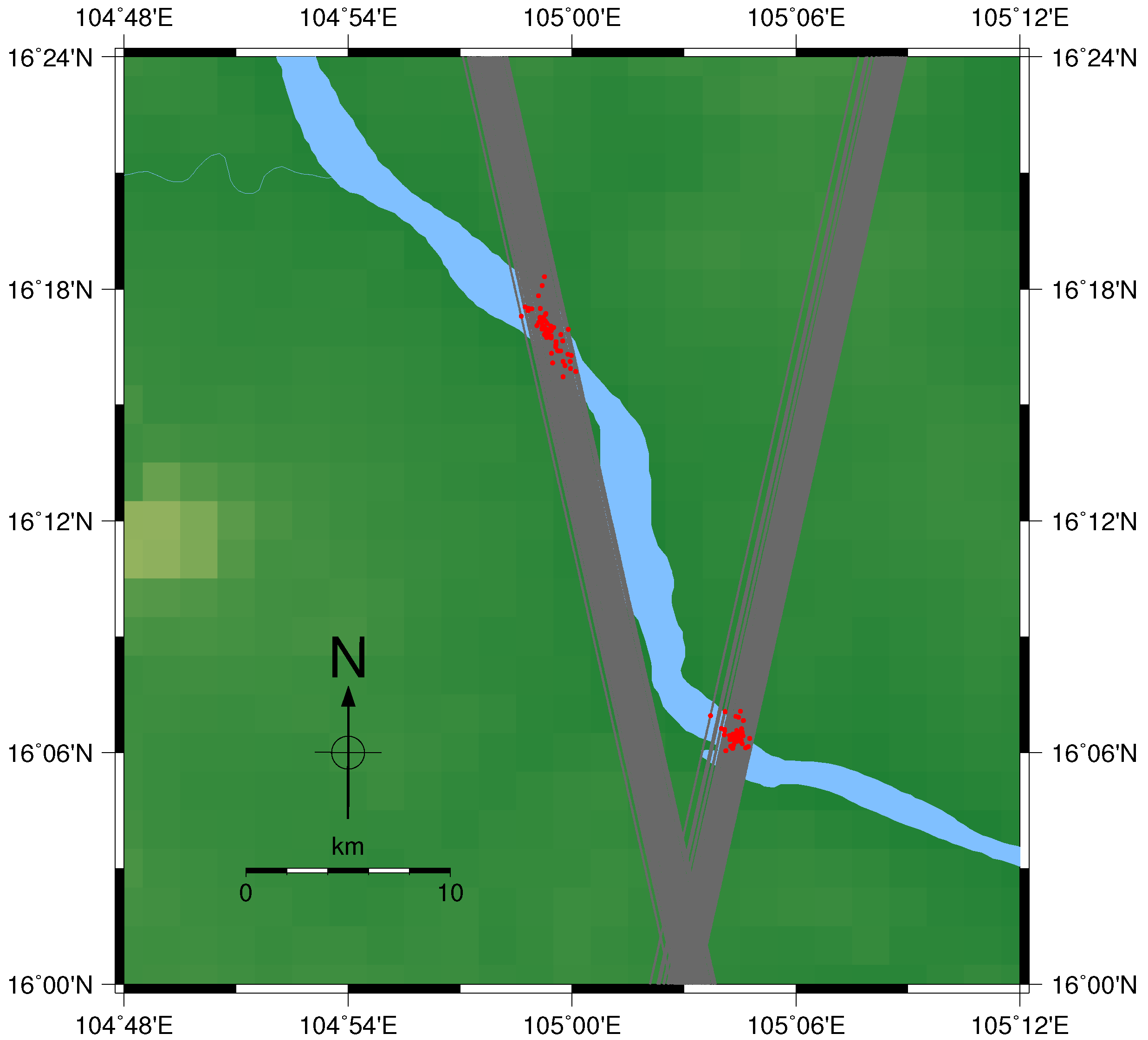
| 013402 | Mukdahan 1 | 39 | Mekong River | 21 | 104.984 | 16.283 | 3220 | 12 | 1.35 | 0.78 | 71 | 0.97 | 0.89 | 67 | 4.61 | 0.25 | 79 | 83 |
| Mukdahan 2 | 60 | Mekong River | 952 | 105.068 | 16.109 | 1000 | 12 | 0.51 | 0.97 | 79 | 0.50 | 0.97 | 77 | 5.47 | 0.16 | 84 | 86 | |
| 120101 | Ban Mixai | 18 | Nam Khan | 666 | 102.3240 | 19.6856 | 90 | 4.50 | 1.79 | 0.58 | 46 | 1.68 | 0.70 | 43 | 3.90 | 0.32 | 67 | 81 |
| 350101 | Ban Keng Done | 42 | Xe Bangfai River | 479 | 105.6986 | 16.3180 | 180 | 14 | 1.44 | 0.78 | 74 | 1.40 | 0.55 | 68 | 6.32 | 0.25 | 80 | 85 |
| 440102 | Voeun Sai 1 | 18 | Tonle San River | 322 | 106.7130 | 13.8421 | 460 | 7 | 0.97 | 0.79 | 73 | 0.34 | 0.88 | 69 | 3.44 | 0.39 | 82 | 84 |
| Voeun Sai 2 | 16 | Tonle San River | 937 | 106.9437 | 14.0426 | 320 | 7 | 0.98 | 0.61 | 63 | 0.89 | 0.59 | 61 | 3.11 | 0.30 | 81 | 85 | |
| 430102 | Siempang | 31 | Tonle Kong River | 479 | 106.2653 | 13.8467 | 430 | 10 | 1.49 | 0.72 | 69 | 1.49 | 0.72 | 69 | 2.29 | 0.44 | 84 | 85 |
6.2. Effects Influencing the Accuracy of the Water-Level Time Series


6.3. Comparison with Other Altimetry Products
6.4. Application of the Hooking Approach to Other Missions

7. Conclusions
Acknowledgments
Author Contributions
Conflicts of Interest
References
- Global Runoff Data Center. Long-Term Mean Monthly Discharges and Annual Characteristics of GRDC Stations; Technical Report; Federal Institute of Hydrology: Koblenz, Germany, 2013. [Google Scholar]
- Morris, C.S.; Gill, S.K. Variation of Great Lakes water levels derived from Geosat altimetry. Water Resour. Res. 1994, 30, 1009–1017. [Google Scholar] [CrossRef]
- Birkett, C. The contribution of TOPEX/POSEIDON to the global monitoring of climatically sensitive lakes. J. Geophys. Res.: Oceans 1995, 100, 25179–25204. [Google Scholar] [CrossRef]
- Birkett, C.M. Contribution of the TOPEX NASA radar altimeter to the global monitoring of large rivers and wetlands. Water Resour. Res. 1998, 34, 1223–1239. [Google Scholar] [CrossRef]
- Berry, P. Two decades of inland water monitoring using satellite radar altimetry. In Proceedings of the Symposium on 15 Years of Progress in Radar Altimetry, Venice, Italy, 13–18 March 2006; Volume 15.
- De Oliveira Campos, I.; Mercier, F.; Maheu, C.; Cochonneau, G.; Kosuth, P.; Blitzkow, D.; Cazenave, A. Temporal variations of river basin waters from Topex/[Poseidon satellite altimetry. Application to the Amazon basin. Comptes Rendus L’Académie Sci.-Ser. IIA-Earth Planet. Sci. 2001, 333, 633–643. [Google Scholar] [CrossRef]
- Chelton, D.B.; Ries, J.C.; Haines, B.J.; Fu, L.L.; Callahan, P.S. Satellite altimetry. Int. Geophys. 2001, 69, i–ii. [Google Scholar]
- Gommenginger, C.; Thibaut, P.; Fenoglio-Marc, L.; Quartly, G.; Deng, X.; Gómez-Enri, J.; Challenor, P.; Gao, Y. Retracking altimeter waveforms near the coasts. In Coastal Altimetry; Benveniste, J., Cipollini, P., Kostianoy, A.G., Vignudelli, S., Eds.; Springer: Berlin, Germany, 2011; pp. 61–101. [Google Scholar]
- Crétaux, J.F.; Jelinski, W.; Calmant, S.; Kouraev, A.; Vuglinski, V.; Bergé-Nguyen, M.; Gennero, M.C.; Nino, F.; Del Rio, R.A.; Cazenave, A.; et al. SOLS: A lake database to monitor in the Near Real Time water level and storage variations from remote sensing data. Adv. Space Res. 2011, 47, 1497–1507. [Google Scholar] [CrossRef]
- Berry, P.; Bracke, H.; Jasper, A. Retracking ERS-1 altimeter waveforms over land for topographic height determination: An expert systems approach. ESA SP 1997, 1, 403–408. [Google Scholar]
- Birkett, C.; Reynolds, C.; Beckley, B.; Doorn, B. From research to operations: The USDA global reservoir and lake monitor. In Coastal Altimetry; Springer: Berlin, Germany, 2011; pp. 19–50. [Google Scholar]
- Schwatke, C.; Dettmering, D.; Bosch, W.; Seitz, F. DAHITI – an innovative approach for estimating water level time series over inland waters using multi-mission satellite altimetry. Hydrol. Earth Syst. Sci. 2015, 19, 4345–4364. [Google Scholar] [CrossRef]
- Frappart, F.; Calmant, S.; Cauhopé, M.; Seyler, F.; Cazenave, A. Preliminary results of ENVISAT RA-2-derived water levels validation over the Amazon basin. Remote Sens. Environ. 2006, 100, 252–264. [Google Scholar] [CrossRef] [Green Version]
- Zhang, M.; Lee, H.; Shum, C.; Alsdorf, D.; Schwartz, F.; Tseng, K.H.; Yi, Y.; Kuo, C.Y.; Tseng, H.Z.; Braun, A.; et al. Application of retracked satellite altimetry for inland hydrologic studies. Int. J. Remote Sens. 2010, 31, 3913–3929. [Google Scholar] [CrossRef]
- Santos da Silva, J.; Calmant, S.; Seyler, F.; Rotunno Filho, O.C.; Cochonneau, G.; Mansur, W.J. Water levels in the Amazon basin derived from the ERS-2 and ENVISAT radar altimetry missions. Remote Sens. Environ. 2010, 114, 2160–2181. [Google Scholar] [CrossRef]
- Kuo, C.Y.; Kao, H.C. Retracked Jason-2 altimetry over small water bodies: Case study of Bajhang River, Taiwan. Mar. Geod. 2011, 34, 382–392. [Google Scholar] [CrossRef]
- Maillard, P.; Bercher, N.; Calmant, S. New processing approaches on the retrieval of water levels in ENVISAT and SARAL radar altimetry over rivers: A case study of the São Francisco River, Brazil. Remote Sens. Environ. 2015, 156, 226–241. [Google Scholar] [CrossRef]
- Calmant, S.; Seyler, F.; Cretaux, J.F. Monitoring continental surface waters by satellite altimetry. Surv. Geophys. 2008, 29, 247–269. [Google Scholar] [CrossRef]
- Santos da Silva, J.; Seyler, F.; Calmant, S.; Rotunno Filho, O.C.; Roux, E.; Araújo, A.A.M.; Guyot, J.L. Water level dynamics of Amazon wetlands at the watershed scale by satellite altimetry. Int. J. Remote Sens. 2012, 33, 3323–3353. [Google Scholar] [CrossRef]
- Frappart, F.; Papa, F.; Marieu, V.; Malbeteau, Y.; Jordy, F.; Calmant, S.; Durand, F.; Bala, S. Preliminary assessment of SARAL/AltiKa observations over the Ganges-Brahmaputra and Irrawaddy Rivers. Mar. Geod. 2015, 38, 568–580. [Google Scholar] [CrossRef]
- Fischler, M.A.; Bolles, R.C. Random sample consensus: A paradigm for model fitting with applications to image analysis and automated cartography. Commun. ACM 1981, 24, 381–395. [Google Scholar] [CrossRef]
- Chen, C.S.; Hung, Y.P.; Cheng, J.B. RANSAC-based DARCES: A new approach to fast automatic registration of partially overlapping range images. IEEE Trans. Pattern Anal. Mach. Intell. 1999, 21, 1229–1234. [Google Scholar] [CrossRef]
- Kim, T.; Im, Y.J. Automatic satellite image registration by combination of matching and random sample consensus. IEEE Trans. Geosci. Remote Sens. 2003, 41, 1111–1117. [Google Scholar]
- Dung, L.R.; Huang, C.M.; Wu, Y.Y. Implementation of RANSAC algorithm for feature-based image registration. J. Comput. Commun. 2013, 1, 46–50. [Google Scholar] [CrossRef]
- Tarsha-Kurdi, F.; Landes, T.; Grussenmeyer, P. Hough-transform and extended ransac algorithms for automatic detection of 3d building roof planes from LiDAR data. In Proceedings of the ISPRS Workshop on Laser Scanning 2007 and SilviLaser 2007, Espoo, Finland, 12–14 September 2007; Volume 36, pp. 407–412.
- Yan, J.; Jiang, W.; Shan, J. Quality analysis on RANSAC-based roof facets extraction from airborne LiDAR data. Int. Arch. Photogramm. Remote Sens. Spat. Inf. Sci. 2012, 1, 367–372. [Google Scholar] [CrossRef]
- Frappart, F.; Do Minh, K.; L’Hermitte, J.; Cazenave, A.; Ramillien, G.; Le Toan, T.; Mognard-Campbell, N. Water volume change in the lower Mekong from satellite altimetry and imagery data. Geophys. J. Int. 2006, 167, 570–584. [Google Scholar] [CrossRef]
- Birkinshaw, S.; O’Donnell, G.; Moore, P.; Kilsby, C.; Fowler, H.; Berry, P. Using satellite altimetry data to augment flow estimation techniques on the Mekong River. Hydrol. Process. 2010, 24, 3811–3825. [Google Scholar] [CrossRef]
- Mekong River Commission (Ed.) Overview of the Hydrology of the Mekong Basin; Mekong River Commission: Vientiane, Lao PDR, 2005.
- Scharroo, R.; Smith, W.H. A global positioning system–based climatology for the total electron content in the ionosphere. J. Geophys. Res.: Space Phys. 2010, 115. [Google Scholar] [CrossRef]
- Boehm, J.; Kouba, J.; Schuh, H. Forecast Vienna Mapping Functions 1 for real-time analysis of space geodetic observations. J. Geod. 2009, 83, 397–401. [Google Scholar] [CrossRef]
- McCarthy, D.D.; Petit, G. IERS Conventions (2003); Technical Report; Verlag des Bundesamtes für Kartographie und Geodäsie: Frankfurt am Main, Germany, 2004. [Google Scholar]
- Förste, C.; Bruinsma, S.; Shako, R.; Abrikosov, O.; Flechtner, F.; Marty, J.C.; Lemoine, J.M.; Dahle, C.; Neumeyer, H.; Barthelmes, F.; et al. A new release of EIGEN-6: The latest combined global gravity field model including LAGEOS, GRACE and GOCE data from the collaboration of GFZ Potsdam and GRGS Toulouse. Geophys. Res. Abstr. 2012, 14, 2821. [Google Scholar]
- Bosch, W.; Dettmering, D.; Schwatke, C. Multi-mission cross-calibration of satellite altimeters: Constructing a long-term data record for global and regional sea level change studies. Remote Sens. 2014, 6, 2255–2281. [Google Scholar] [CrossRef]
- Benveniste, J.; Baker, S.; Bombaci, O.; Zeli, C.; Venditti, P.; Zanife, O.; Soussi, B.; Dumont, J.; Stum, J.; Milagro-Perez, M. ENVISAT RA-2/MWR Product Handbook, Issue 2.2; Technical Report; PO-TN-ESR-RA-0050; European Space Agency: Frascati, Italy, 2007.
- Koch, K.R. Parameter Estimation and Hypothesis Testing in Linear Models; Springer Science & Business Media: Berlin, Germany, 1999. [Google Scholar]
- Gupta, A.; Liew, S.C. The Mekong from satellite imagery: A quick look at a large river. Geomorphology 2007, 85, 259–274. [Google Scholar] [CrossRef]
- NASA. Landsat 7 Science Data Users Handbook; Technical Report; National Aeronautics and Space Administration: Washington DC, USA, 2011.
- Schwatke, C.; Dettmering, D.; Börgens, E.; Bosch, W. Potential of SARAL/AltiKa for inland water applications. Mar. Geod. 2015, 38, 626–643. [Google Scholar] [CrossRef]
© 2016 by the authors; licensee MDPI, Basel, Switzerland. This article is an open access article distributed under the terms and conditions of the Creative Commons by Attribution (CC-BY) license (http://creativecommons.org/licenses/by/4.0/).
Share and Cite
Boergens, E.; Dettmering, D.; Schwatke, C.; Seitz, F. Treating the Hooking Effect in Satellite Altimetry Data: A Case Study along the Mekong River and Its Tributaries. Remote Sens. 2016, 8, 91. https://0-doi-org.brum.beds.ac.uk/10.3390/rs8020091
Boergens E, Dettmering D, Schwatke C, Seitz F. Treating the Hooking Effect in Satellite Altimetry Data: A Case Study along the Mekong River and Its Tributaries. Remote Sensing. 2016; 8(2):91. https://0-doi-org.brum.beds.ac.uk/10.3390/rs8020091
Chicago/Turabian StyleBoergens, Eva, Denise Dettmering, Christian Schwatke, and Florian Seitz. 2016. "Treating the Hooking Effect in Satellite Altimetry Data: A Case Study along the Mekong River and Its Tributaries" Remote Sensing 8, no. 2: 91. https://0-doi-org.brum.beds.ac.uk/10.3390/rs8020091