Article

Estimation of Land Surface Temperature through Blending MODIS and AMSR-E Data with the Bayesian Maximum Entropy Method

State Key Laboratory of Remote Sensing Science, Research Center for Remote Sensing and GIS, and School of Geography, Beijing Normal University, Beijing 100875, China
*
Author to whom correspondence should be addressed.
Submission received: 17 November 2015 / Revised: 21 January 2016 / Accepted: 25 January 2016 / Published: 29 January 2016
(This article belongs to the Special Issue Satellite Climate Data Records and Applications)

Abstract

:
Land surface temperature (LST) plays a major role in the study of surface energy balances. Remote sensing techniques provide ways to monitor LST at large scales. However, due to atmospheric influences, significant missing data exist in LST products retrieved from satellite thermal infrared (TIR) remotely sensed data. Although passive microwaves (PMWs) are able to overcome these atmospheric influences while estimating LST, the data are constrained by low spatial resolution. In this study, to obtain complete and high-quality LST data, the Bayesian Maximum Entropy (BME) method was introduced to merge 0.01° and 0.25° LSTs inversed from MODIS and AMSR-E data, respectively. The result showed that the missing LSTs in cloudy pixels were filled completely, and the availability of merged LSTs reaches 100%. Because the depths of LST and soil temperature measurements are different, before validating the merged LST, the station measurements were calibrated with an empirical equation between MODIS LST and 0~5 cm soil temperatures. The results showed that the accuracy of merged LSTs increased with the increasing quantity of utilized data, and as the availability of utilized data increased from 25.2% to 91.4%, the RMSEs of the merged data decreased from 4.53 °C to 2.31 °C. In addition, compared with the filling gap method in which MODIS LST gaps were filled with AMSR-E LST directly, the merged LSTs from the BME method showed better spatial continuity. The different penetration depths of TIR and PMWs may influence fusion performance and still require further studies.

Graphical Abstract

1. Introduction

Land surface temperature (LST) plays a significant role in terrestrial environmental conditions [1]. As one of the main parameters of surface energy balances, it deeply influences the terrestrial biophysical process, including evapotranspiration, plant respiration, and photosynthesis. It has been extensively used in research areas such as global climate warming, applied meteorology, agriculture, hydrology, and ecology [2,3,4,5].
The conventional method of monitoring LST based on ground sites is limited by the uncertainties caused by measurement inconsistencies and bias over large areas [6]. In contrast, satellite remote sensing provides ways to estimate LST at dense spatial sampling intervals and large scales. Various methods for estimating LST from remote sensing data have been extensively implemented since the 1990s [7,8,9,10,11,12,13,14,15]. Among them, most can be classified into two main methods. The first is based on thermal infrared (TIR) remotely sensed data, such as single channel algorithms, temperature and emissivity separation algorithms, and split-window algorithms, which have been used for sensors with one, two or multiple TIR channels, respectively [16,17,18,19,20]. The other is based on passive microwave (PMW) remotely sensed data, including the empirical and statistical, semi-empirical and physical methods, in which the lower-frequency (≤37 GHz) brightness temperatures (TB) and surface emissivities from passive microwave radiometry are usually used [21,22,23,24,25,26,27,28]. For the former method, the retrieved LSTs are mostly within a relatively fine spatial scale; for example, the Moderate Resolution Imaging Spectroradiometer (MODIS) sensor aboard the Aqua satellite platforms provide daily, eight-day, and monthly LST products at 1 km (near) and 6 km (near) resolution. However, TIR remote sensing data are greatly influenced by atmospheric effects and cloud cover contamination. More than 60% of the areas in the MODIS LST products are contaminated by weather effects, especially cloud cover [29]. Thus, various applications based on MODIS data are restricted to clear-sky conditions [30,31]. For the latter method, because PMW radiation from the land surface can penetrate atmosphere and clouds, few instances of missing data appear in the retrieved LST. Nevertheless, LSTs derived from PMW remotely sensed data have a relatively coarse (~25 km) spatial resolution. In addition, because the surface emissivity at PMW bands is sensitive to land surface properties and difficult to measure, the inversion accuracy is always limited and lower than that of TIR methods [32].
To meet the demands of applications in surface energy balance research, applied meteorology, and other fields, many methods have been developed in previous studies to obtain complete and high-quality LST data both spatially and temporally [33,34,35,36,37,38]. Temporal interpolation is a straightforward method to fill the MODIS LST product gaps. However, the accuracy is limited by the uncertainty of the regression equations; only the mean annual LST is usually used in such applications [33,34]. Another method is to fill the LST retrieval gaps with ancillary meteorological data [35]. However, uncertainties during resampling or simple local averaging are inevitable, which should be attributed to the coarse spatial resolution (~100 km) of the global meteorological data [36,37]. Beyond that, a simple pixel-wise empirical regression method was recently implemented by combining the TIR LST and PMW TB products [38]. Although the results show reasonable accuracy (4–5 K), the process of downscaling PMW TB (~25 km) to sub-grid cell levels (~5 km) may not be suitable, particularly in downscaling 25 km resolution to 1 km. Because there is a large gap between the two spatial resolutions, the spatial variability within coarser pixels should not be ignored. Therefore, to satisfy the application requirements at regional and local scales, a new strategy is needed.
As one of the spatiotemporal geostatistical nonlinear methodologies, the Bayesian Maximum Entropy (BME) method can theoretically integrate data from different sources with different accuracies [39,40]. It has not only been used in environmental risk assessment, soil property mapping, et al. [41,42,43,44,45], but it has also been successfully applied in the combination of MODIS sea surface temperature (SST) with AMSR-E SST [46]. In this study, we investigated the feasibility of the BME method to estimate spatially and temporally complete LST time series at a relatively fine spatial resolution. The goals of this article are to (1) demonstrate the possibility of spatially and temporally complete LST reconstruction; (2) systematically examine how the accuracy of merged LST varies with the amount of data used in the BME estimation procedure; and (3) illustrate the advantages of the BME method in contrast with the gap filling method.

2. Study Area and Data
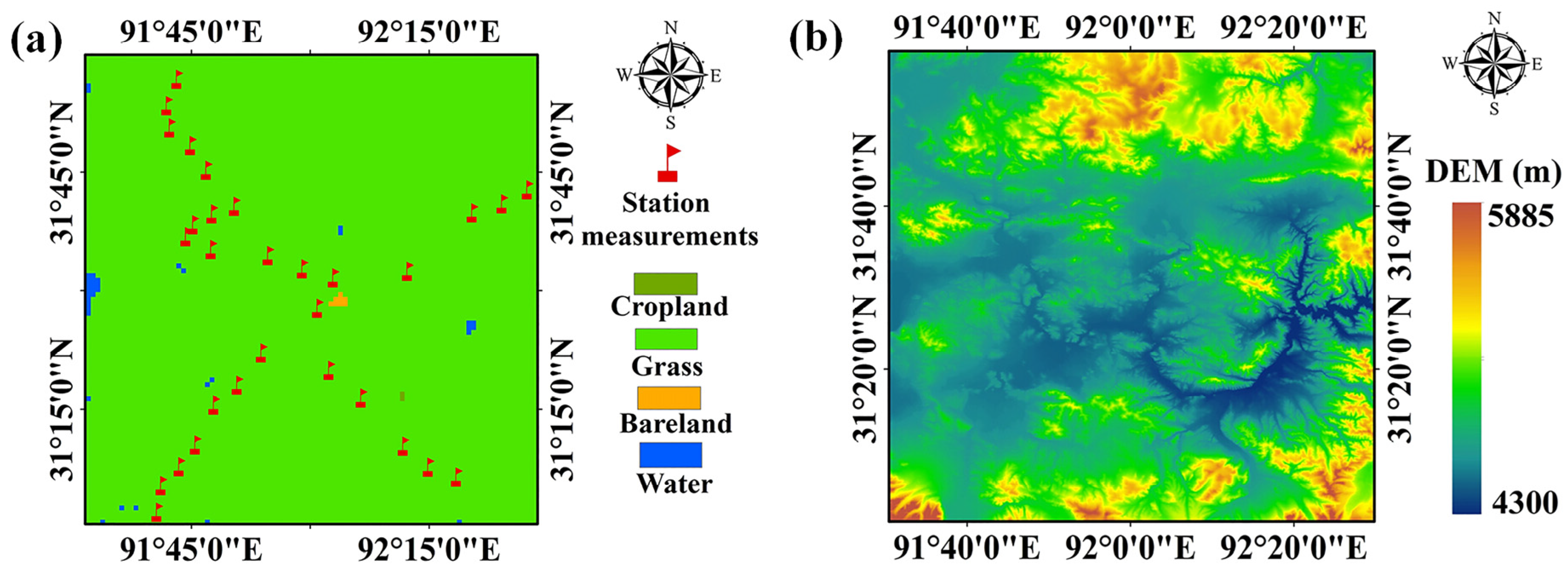
2.1. Study Area

The Tibetan Plateau (TP), with an area of approximately 2.5 × 10 6   km 2 , is the highest plateau in the world. Its temperature, water and energy dynamics have a significant impact on climate change in Asia [47,48]. Our study area is in the central TP around Naqu City (31°–32°N, 91.5°–92.5°E), which has an area of 100 2   km 2 and an average elevation of 4650 m above sea level. Overview of the study area was shown in Figure 1. This area is mostly covered by short and sparse grasses in summer, and it has a cold and semiarid climate. The terrain is relatively flat with rolling hummocks and hills. Land cover data were downloaded from http://www.globallandcover.com/home/background.aspx. The elevation dataset was provided by the International Scientific & Technical Data Mirror Site, the Computer Network Information Center and the Chinese Academy of Sciences (http://www.gscloud.cn).
Figure 1. Overview of the study area: (a) land-cover map and station locations; (b) DEM.
Remotesensing 08 00105 g001

2.2. Data

2.2.1. Satellite-Derived LST Products

The LST products used in this study were derived from the MODIS and AMSR-E sensors aboard NASA’s Aqua satellite. Their specifications are given in Table 1.
Table 1. Specifications of the satellite-derived LST products used in this study.
MODIS LSTAMSR-E LST
Time rangeFrom 1 August 2010 to 28 July 2011
Temporal resolutionDaily (1:30 A.M. local time)
Space range91.5°E–92.5°E, 31°N–32°N
Spatial resolutionApprox. 1 kmApprox. 25 km
ProjectionSinusoidalAlbers Conical Equal Area
The MODIS LSTs provided by the Land Processes Distributed Active Archive Center (LP DAAC) site (https://lpdaac.usgs.gov/) were retrieved from measurements in the thermal infrared channels (10.780–11.280 μm and 11.770–12.270 μm) based on the use of the day-night split-window algorithm [16]. The MODIS 1 km LST product has been cross-compared and validated against ground-based temperature measurements over homogeneous surfaces, and the results showed that the accuracy could be better than 1 K in clear-sky conditions [49].
The AMSR-E daily LST data used in this study were derived from the PMW TB product (provided by the National Snow and Ice Data Center (NSIDC), http://gcom-w1.jaxa.jp/sftp_man.html) based on the temporal land cover-based look-up table (TL-LUT) method [32]. Compared to other statistical retrieval methods, one major advantage is that the variations of the physical characteristics of the land surface and their dynamic influences were considered in this method. Compared with in situ measured LSTs at four sites without urban warming in the TP, the standard errors of estimation between the estimated AMSR-E LST and in situ measured LST range from 3.1 K to 4.5 K at night [32].
It is important to minimize the influence factors in the processing procedure. Due to the warming effect of sunshine, using daytime LST may increase the uncertainty of the validation process. Therefore, the night-time LSTs from Aqua MODIS and AMSR-E at a local time 1:30 AM were selected for the blending process. In addition, for the convenience of calculation, the MODIS and AMSR-E LST products were uniformly transformed into geographic Lat/Lon projections and resampled to spatial resolutions of 0.01° and 0.25°, respectively.

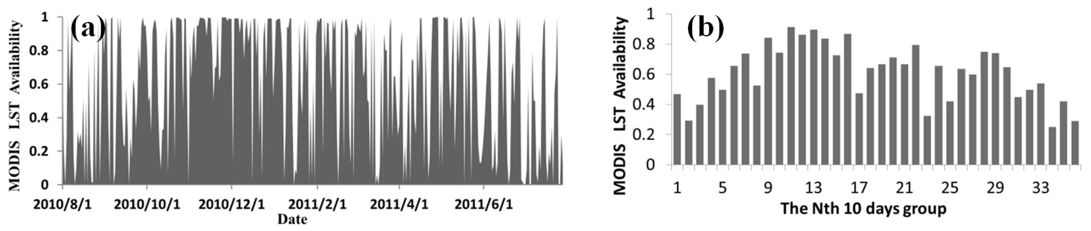
2.2.2. Data Used in This Study

Before conducting the merging process, we first checked the availability of MODIS LST products. The availability is measured by valid LST pixels divided by all LST pixels. As shown in Figure 2, the daily availability of MODIS LST changed from 0% to 100%, and the 10-day averaged availability during the period from 1 August 2010 to 28 July 2011 varied from 25.2% to 91.4%. The availability of the AMSR-E LST product was also checked, and few instances of missing data occurred. Seven periods of data were selected based on the 10-day averaged availability shown in Figure 2b, and the dates and availabilities are given in Table 2. They were used to examine how the accuracy of merged LST varies with the amount of data used in the BME estimation procedure. Though the total data (only 70 days) used in the estimation procedure is small, both the availability (from 25.2% to 91.4%) and temperature range (from 250 K to 290 K) were considered in the selection process. Thus, the data in the seven selected periods could effectively represent the data features of the whole year.
Figure 2. MODIS LST availability in the study area: (a) Daily availability (from 1 August 2010 to 28 July 2011); (b) 10-day grouped averaged availability (from 1 August 2010 to 26 July 2011).
Remotesensing 08 00105 g002
Table 2. Dates and availabilities of the selected data.
The Nth Period (Date)MODIS LST AvailabilityAMSR-E LST Availability
Period 134 (from 27 June to 6 July, 2011)25.2%76.3%
Period 223 (from 9 March to 18 March, 2011)32.4%87.5%
Period 317 (from 8 January to 17 January, 2011)47.5%86.3%
Period 404 (from 31 August to 9 September, 2010)57.6%95.6%
Period 507 (from 30 September to 9 October, 2010)73.7%85.6%
Period 614 (from 9 December to 18 December, 2010)83.6%85.0%
Period 711 (from 9 November to 18 November, 2010)91.4%95.0%

2.2.3. Comparison Data
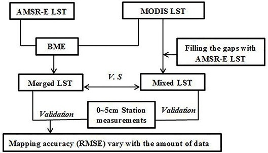
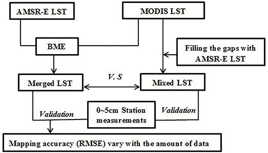
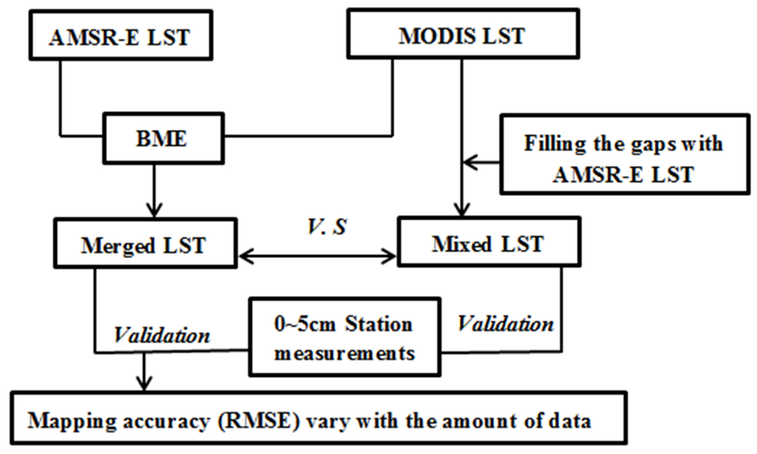
A multiscale monitoring network that consists of 69 stations was established on the central TP to measure moisture and temperature at four soil depths (0–5, 10, 20, and 40 cm) in 2010–2012. The dataset was provided by the Data Assimilation and Modeling Center for Tibetan Multi-spheres at the Institute of Tibetan Plateau Research, Chinese Academy of Sciences. Readers are referred to Yang et al. [50] for more information about this network. In this study, only the temperature measurements at soil depths of 0–5 cm between August 2010 and August 2011 for 38 stations (as shown in Figure 1a) were used to perform the comparison.

3. Methodology

To achieve the three goals of this article as mentioned above, a flowchart was designed, as shown in Figure 3. First, the BME method was applied to merge the seven groups of LST data derived from the infrared (MODIS) and microwave (AMSR-E) satellites. Second, the accuracy of the merged LST was analyzed with the amount of data used in the estimated procedure. Finally, we compared the merged LST with the BME method and the mixed LST from the gap filling method to illustrate their characteristics. In this work, the simple gap filling method as termed here used the AMSR-E LST to fill the gaps of the MODIS LST directly. In contrast, the BME method is more complicated. As a spatiotemporal geostatistical methodology, the BME method can perform interpolation with uncertain data through a probabilistic approach. In this section, the basic knowledge about the spatiotemporal random field is briefly described. The major steps in applying the BME algorithm are then introduced.
Figure 3. Schematic flow diagram for the blending MODIS and AMSR-E LST using the BME method.
Remotesensing 08 00105 g003

3.1. Spatiotemporal Random Field
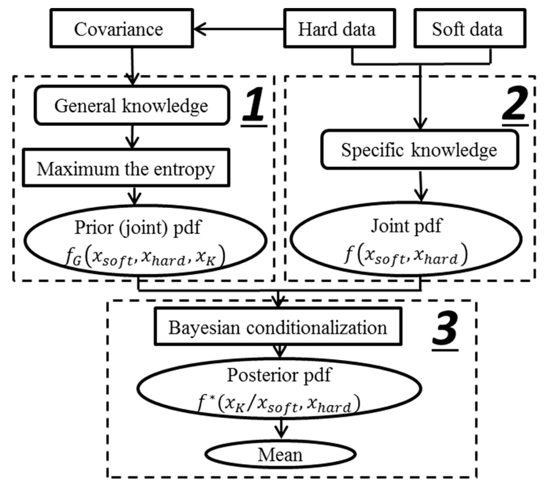
The distribution of a natural variable (in this case, LST) can be represented in terms of a spatiotemporal random field (S/TRF), X ( p ) , which takes values at points p = ( s , t ) in a space–time domain, where s = ( s 1 , s 2 ) represents the spatial location and t denotes the time [51]. In a given S/TRF, a random variable x i can acquire any one value χ i from a distribution of values, and it is fully described by its cumulative distribution function (cdf) or probability density function (pdf). The random field X ( p ) is a collection of random variables x m a p = [ x 1 , , x m , x k ] at points P i ( i = 1 , , m, k). It is completely described by the multivariate cdf:
F x ( χ 1 , , χ m , χ k ) = P r o [ x 1 χ 1 , x m χ m , x k χ k ]
Its derivative with respect to χ m a p = [ χ 1 , , χ m , χ k ] is the multivariate pdf:
f x ( χ 1 , , χ m , χ k ) = F x ( χ 1 , , χ m , χ k )
In general, S/TRF can be characterized by its mean function, m x ( p ) = X ( p ) ¯ (the bar denotes stochastic expectation), or its covariance function, c x ( p , p ) = [ X ( p ) X ( p ) ¯ ] [ X ( p ) X ( p ) ¯ ] ¯ . The mean function of the S/TRF characterizes trends and systematic structures in space/time, and the covariance function expresses spatiotemporal correlations and dependencies. If both spatial and temporal trends are absent, the S/TRF is spatially homogeneous and temporally stationary; in this case, the mean function is constant, and the covariance function depends only on the spatial lag, r = s s' , and the temporal lag, τ = t t' , between any two points, p = ( s , t ) and p = ( s , t ) .
In this study, the spatial distribution of LST at a given time x t ( s ) can be decomposed into a deterministic mean trend μ t ( s ) and a zero-mean residual field ε t ( s ) , as   x t ( s ) = μ t ( s ) + ε t ( s ) . It is necessary to quantify and remove the trends before investigating the autocorrelation structure of the data [52]. To remove the mean trend of   μ t ( s ) , the Gaussian kernel smoothing method was applied to the dataset. The kernel searches for neighboring data within 0.25° grid ranges and extracts the trend using a 25 × 25 moving window in the MODIS LST data. The moving window was chosen here for two reasons. Firstly, the MODIS LSTs show a close relation in a 0.25° by 0.25° region. Secondly, the size of a PMW LST pixel is equal to that of a 25 × 25 MODIS pixel. This is convenient for the subsequent calculation.
After removing the surface trends of MODIS LSTs and AMSR-E LSTs, Normal score transformation was applied to form the residual components, ε t ( s ) , with a Gaussian distribution [53]. Point pairs of ε t ( s )   at specific distances were used to calculate the covariance. To describe the inherent spatial variability and estimate the entire random field, we model the covariance functions of ε t ( s ) of LSTs with a nested covariance model, with two exponential models and two spherical models, according to the least squares method:
C = c 1 exp ( 3 s a s 1 ) +   c 1 s p h ( 1 ( 3 t 2 a t 1 t 3 2 a t 1 ) ) +   c 2 s p h ( 1 ( 3 s 2 a s 2 s 3 2 a s 2 ) ) + c 2 exp ( 3 t a t 2 )
where c 1 and c 2 are the partial sill variances of the two exponential and two spherical models, respectively. a s 1   and a s 2 are the spatial ranges, and a t 1 and a t 2   are the time ranges, respectively. The range is a type of distance parameter often known as the “correlation length.” If the distance (s) or time (t) is greater than the range, the spatial dependence or time dependence would disappear.

3.2. BME Method

The S/TRF was characterized by physical knowledge bases, which included a general knowledge base G and a specific knowledge base S. G is considered general in the sense that it is universally applicable to all entities, which may include physical laws, scientific theories, or statistical moments. S can be divided into 2 groups: hard data and soft data. Hard data are those data with no error or few errors. In contrast, soft data are the data associated with different sources of uncertainties. In this study, MODIS LST has a higher spatial resolution compared with AMSR-E LST, and it can better reflect the details of the LST spatial features. Thus, MODIS LST can be considered as exact hard data, and AMSR-E LST can be considered as soft data. Both G and S are used in the BME analysis. The major steps of the BME algorithm are described briefly as follows (Figure 4).
Figure 4. Major steps of the BME algorithm.
Remotesensing 08 00105 g004

A. Step 1

The first step is known as the prior stage. The task of this step is to obtain the prior pdf from G. G used in this study is the covariance moment of the MODIS LST. Due to the lack of probabilities of unknown points, the real prior pdf was replaced by the joint pdf without specific information. For a regional variable x m a p , which consists of a vector of points, including values at soft data points x s o f t , values at hard data points x h a r d ,   and the unknown value at estimation point   x K , the joint pdf f G ( x s o f t , x h a r d , x K )   can be written as f G ( x m a p ) . Based on Shannon’s information criterion (Shannon, 1948), the regional information entropy can be calculated by the following equation:
ϕ [ x m a p , f G ( x m a p ) ] = f G ( x m a p ) log [ f G ( x m a p ) ]
Generally, with greater entropy, a greater amount of information is obtained, and the results are closer to the actual situation. To guarantee that the most abundant information was blended into the estimation process, the Lagrange multiplier, λ α ,   is introduced to maximize the entropy with the constraint of variance:
L [ f G ( x m a p ) ] = f G ( x m a p ) log [ f G ( x m a p ) ] d x m a p a N λ α [ g a ( x m a p ) f G ( x m a p ) d x m a p E [ g a ( x m a p ) ] ]
where L [ f G ( x m a p ) ]   is the object function, g a ( x m a p ) is a set of function covariance moments in LST blending, and E [ g a ( x m a p ) ] is the expected value of   g a ( x m a p ) .
The joint pdf can then be obtained by the following equation:
f G ( x s o f t , x h a r d , x K ) = f G ( x m a p ) = exp ( a = 1 N λ α g a ( x m a p ) ) / exp ( a = 1 N λ α g a ( x m a p ) ) d x m a p

B. Step 2

The second step is known as the middle stage. The task of this step is to use a proper form to express S. As mentioned above, in this study, MODIS LST was considered as hard data, with positions in the centers of pixels at 0.01° resolution. Meanwhile, AMSR-E LST was considered as soft data because of its uncertainty, with positions in the centers of pixels at 0.25° resolution. The joint pdf f ( x s o f t , x h a r d )   of hard data and soft data could then be obtained.
In addition, to solve the multiscale problem, soft data were expressed in terms of a Gaussian probability distribution. The mean and variance of the Gaussian distribution were determined with the error model [46]. Readers are encouraged to refer to Li et al. [46] for details about the error model.

C. Step 3

The final step is also called the posterior stage. In this step, the specific information was added into the process. The posterior pdf, f * ( x K / x s o f t , x h a r d ) , can be obtained based on the Bayesian rule:
f * ( x K / x s o f t , x h a r d ) = f G ( x s o f t , x h a r d , x K ) / f ( x s o f t , x h a r d )
Finally, the mean at the estimation point x ¯ K / k can be extracted from Equation (8):
x ¯ K / k = x K f k ( x K ) d x k

4. Results

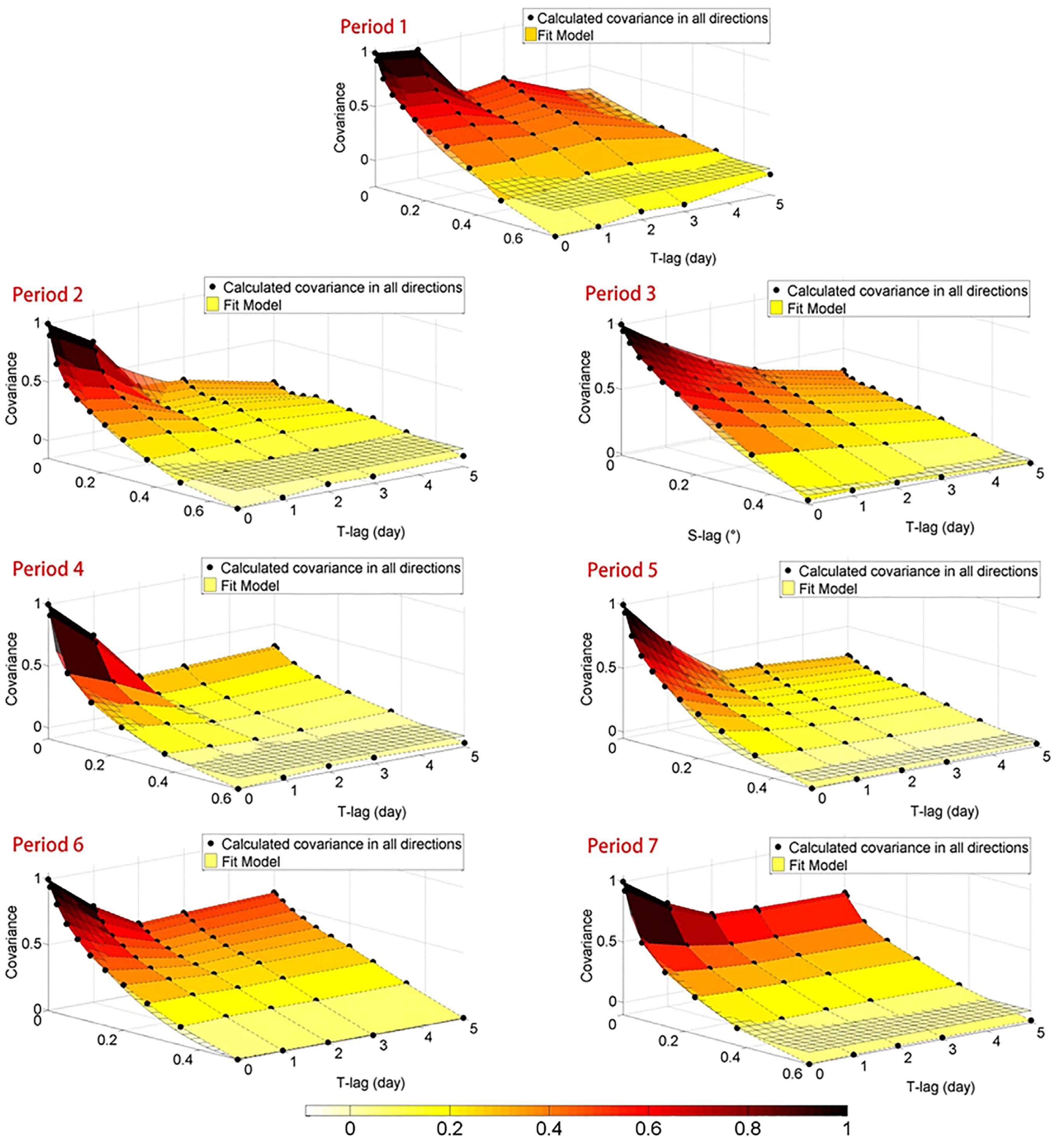
4.1. Modeling the Spatial Covariance Models

We modeled the spatial and temporal variation of LSTs with Equation (3) for each 10-day period. The calculated covariance for all directions and fit models for each period are shown in Figure 5. The parameters of the covariance functions are given in Table 3. The covariance model in period 1 has a partial sill c 1 of 0.4 and a spatial range a s 1 of 0.18° (196 pixels at a resolution of 0.01°), as well as a temporal range a t 1 of 4 days. The other nested model in period 1 has a partial sill c 2 of 0.6, a spatial range a s 2 of 0.6° (2500 pixels at a resolution of 0.01°), and a temporal range a t 2 of 12 days. The covariance model in period 1 indicates that the lower variability of local-scale LSTs has a spatial range of 0.18° (temporal range of 4 days) compared with the variability of 0.6, and it has a spatial range of 0.6° (temporal range of 10 days). The spatial structure could be explained by the discontinuity of land surface parts, and the temporal structure may be influenced by wind, precipitation and other factors. Parallel spatial and temporal structures occur in other periods. One point that should be noted was that for one period, only 10 days of data were used to establish the model; the spatial range a t 2 was fitted by the covariance variation tendencies at each period. In addition, the variations of calculated covariance in periods 3, 4, 5, 6, and 7 were smoother than those in periods 1 and 2, which can be attributed to the influence of the serious lack of data in periods 1 and 2.
Figure 5. The calculated covariance in all directions and the corresponding fit models for different periods (from period 1 to 7).
Remotesensing 08 00105 g005
Table 3. Parameters of the covariance models.
No.Exponential (s)/Spherical (t)Spherical (s)/Exponential (t)
c 1 a s 1 a t 1 c 2 a s 2 a t 2
Period 10.40.1840.60.612
Period 20.40.2040.60.520
Period 30.40.4040.60.625
Period 40.40.2030.60.520
Period 50.40.2540.60.625
Period 60.40.3050.60.640
Period 70.40.2050.60.640

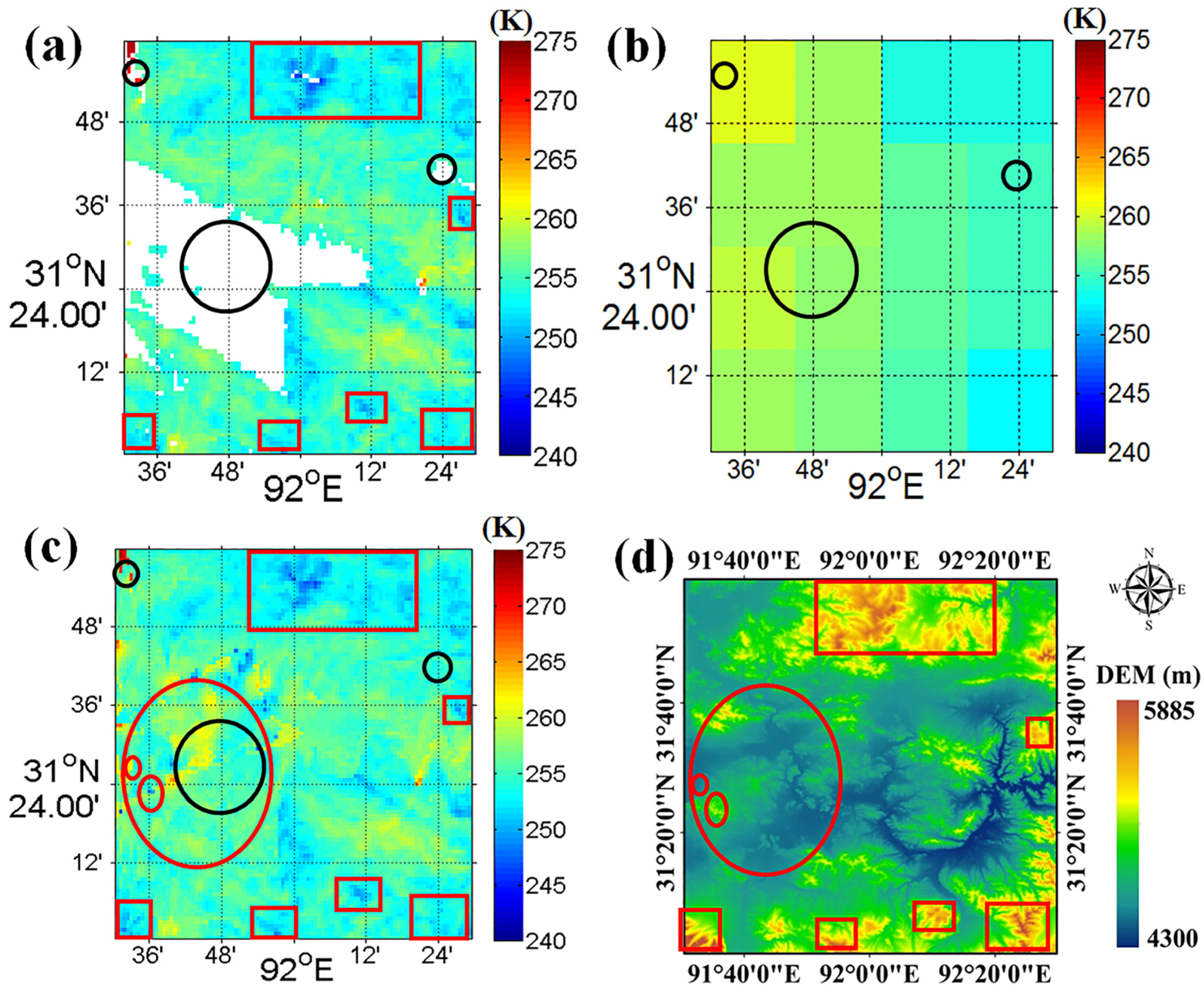
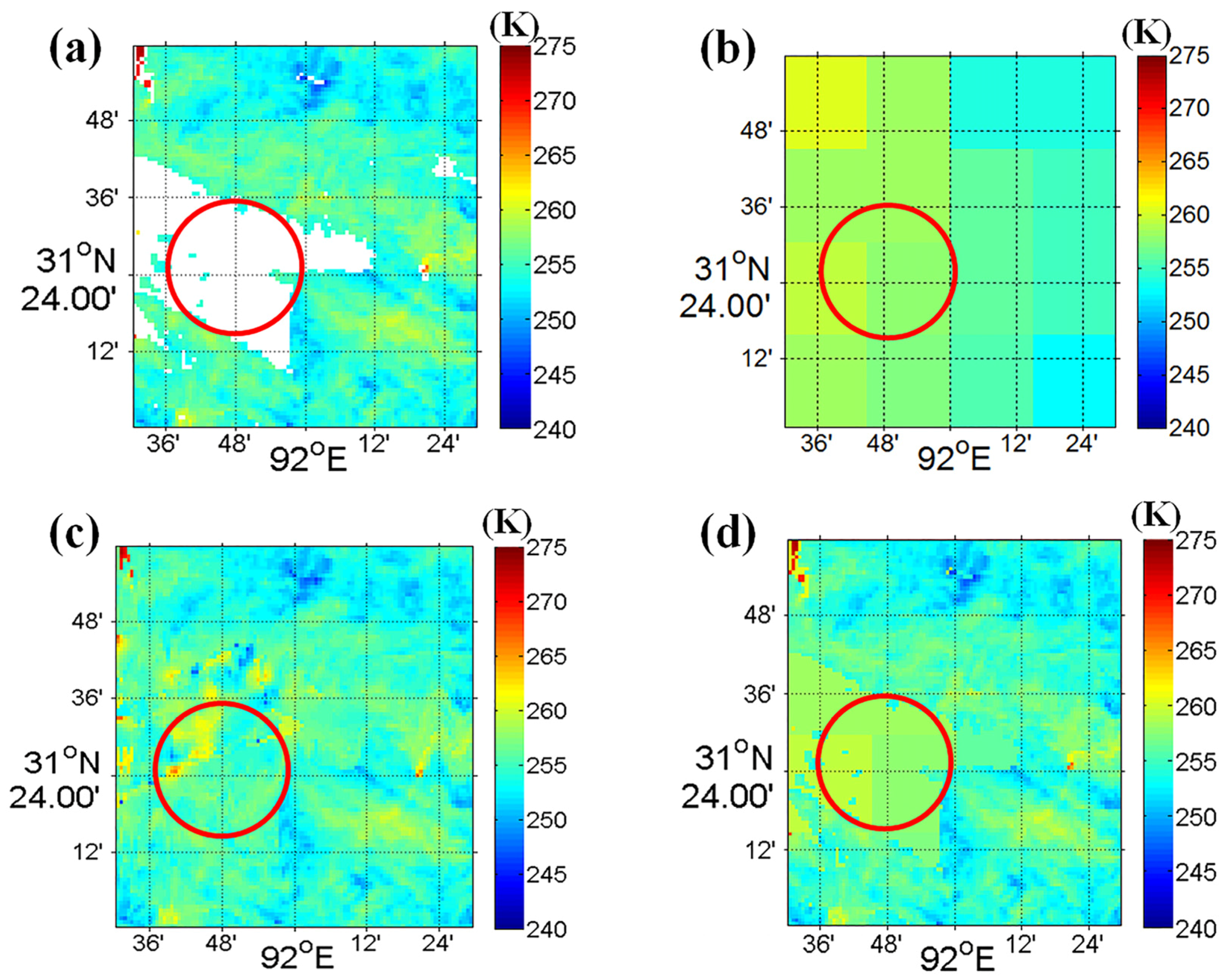
4.2. Availability and Spatial Distribution of the MODIS LSTs, AMSR-E LSTs, and Merged LSTs

Both spatially and temporally complete LSTs are characterized by availability statistics. The averaged availability of MODIS LSTs, AMSR-E LSTs, and merged LSTs in periods 1 through 7 has been examined and listed in Table 4. The availability was computed by valid LST pixels divided by all LST pixels. After the merging process, the availability of merged LSTs at each period reached 100%.
Table 4. Availability of MODIS LSTs, AMSR-E LSTs, and merged LSTs.
NoMODIS LSTAMSR-E LSTMerged LST
Period 125.2%76.3%100%
Period 232.4%87.5%100%
Period 347.5%86.3%100%
Period 457.6%95.6%100%
Period 573.7%85.6%100%
Period 683.6%85.0%100%
Period 791.4%95.0%100%
LSTs on 17 November 2010 (period 7) for the AMSR-E, MODIS, and merged LSTs are shown in Figure 6a–c, respectively. The blank areas in Figure 6a indicate that the MODIS LSTs were missing. From the comparisons of Figure 6a,c, it can be observed that in the areas where MODIS LSTs exist (especially the six areas marked with red rectangular frames), the merged LSTs in Figure 6c retain the details of the MODIS LSTs in Figure 6a. Additionally, in the areas where the MODIS data are missing (especially the three areas marked with black round frames), the merged LSTs in Figure 6c contain both the spatial trend of the MODIS LSTs in Figure 6a and the features of the AMSR-E LSTs in Figure 6b.
In addition, the MODIS LSTs and merged LSTs also show broadly similar spatial distribution characteristics to the elevation diagram. As seen in Figure 6d, the elevations in the six areas of the red rectangular frames are much higher than the surrounding areas. Generally, temperature declines with increasing elevation. Thus, lower LSTs occurred along the mountains, as shown in Figure 6a,c. Moreover, the merged LSTs in the areas where MODIS has missing data also show rough agreement with the elevation data, as shown in the three red oval frames in Figure 6c,d. These features demonstrate that the merged LSTs were reasonably distributed. Because LST was influenced by many factors, such as cloud cover, precipitation, and wind, the merged LST did not strictly correspond to the distribution of elevation for all areas.
Figure 6. The spatial distribution of LSTs (in Kelvin) and elevation: (a) MODIS LST; (b) AMSR-E LST; (c) merged LST; and (d) elevation in the study area on 17 November 2010.
Remotesensing 08 00105 g006

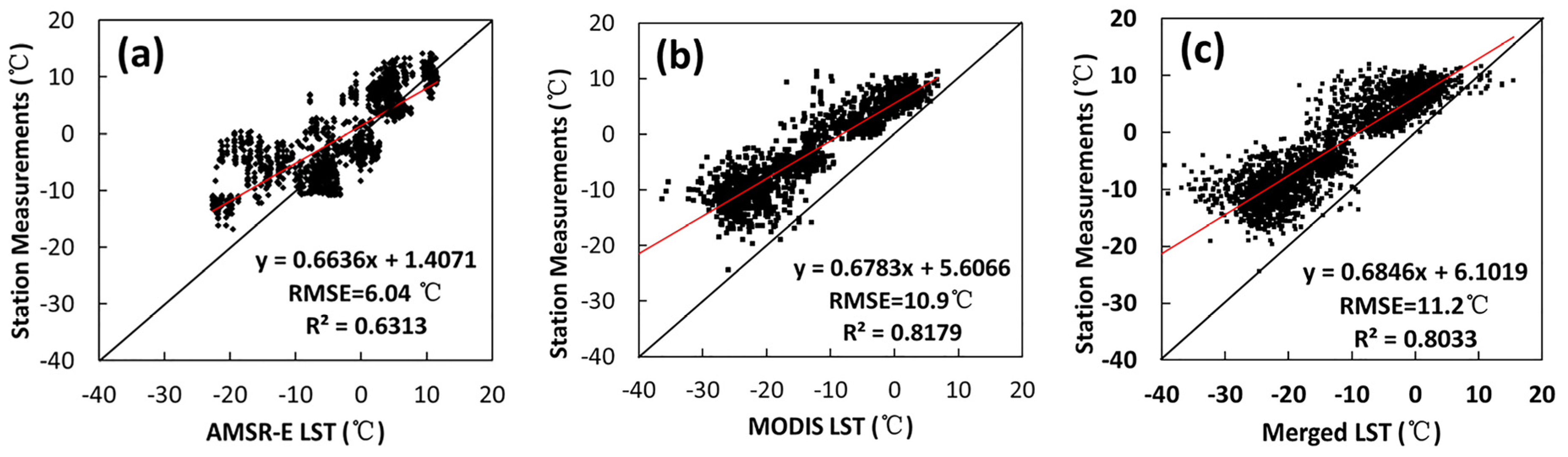
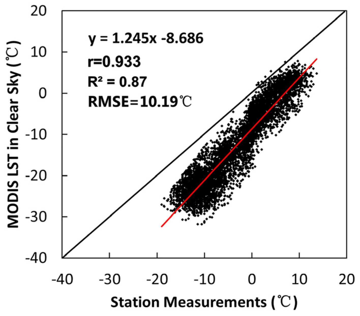
4.3. Comparison of Merged LSTs with the 0–5 cm Soil Temperature

The merged LSTs in seven periods were validated with the soil temperatures at depths of 0–5 cm at 38 stations. As shown in Figure 7c, the merged LSTs showed a strong correlation with the station measurements, with correlation coefficients of 0.896 and R 2 = 0.8033 . However, the RMSE between them is very large, with a value of 11.2 °C. This should be attributed to the fact that the land surface temperature approached the temperature at 0 cm or above 0 cm soil depth, which differed from the soil temperature at depths of 0–5 cm.
Figure 7. Comparison of the station measurements (0–5 cm soil temperatures) with the corresponding LSTs: (a) AMSR-E LST; (b) MODIS LST; and (c) merged LST for the seven periods.
Remotesensing 08 00105 g007
To solve this discrepancy, we also performed comparisons of MODIS LSTs and AMSR-E LSTs with station measurements in the seven periods. As shown in Figure 7a,b, both MODIS LSTs and AMSR-E LSTs present similar tendencies to merged LSTs compared with station measurements. The correlation between MODIS and station measurements is greater than that for AMSR-E, with correlation coefficients of 0.904 and 0.795, respectively. This is mainly caused by the significant difference of MODIS and AMSR-E spatial resolutions compared to in situ measurements. Because MODIS spatial resolution is much finer than that of AMSR-E, higher correlation between the MODIS LST and merged LST was expected because of the high spatial variability of LSTs. Meanwhile, the RMSE of AMSR-E was smaller than that of MODIS, which can be attributed to the fact that, compared to TIR, the PMW radiation exhibited stronger penetration and could detect slightly deeper temperatures.
The merged LSTs by the BME method were mainly estimated from the spatial-temporal LST trend extracted from the hard data (MODIS LST). In addition, both the merged LST and MODIS LST have the same spatial resolution. Therefore, compared with the station measurements, the merged LST showed similar results (correlation coefficient and RMSE) with the MODIS LST. Although all of the LSTs in the seven periods were used in the comparison, the number of data pairs (N) used in the statistics for Figure 7a–c was different. In Figure 7c, the availability of merged LST is 100%, with N = 2660. In Figure 7a, the station measurements were averaged according to the position of AMSR-E pixels, with N = 672. However, in Figure 7b, only the MODIS data of the seven periods were applied to the comparison, with N = 1592. When the MODIS LST data are lacking, the exact spatial-temporal trend of LST could not be obtained, and outliers were found in the predicted values (especially in the area where MODIS LST is missing). The RMSE of the merged LST shown in Figure 7c is slightly larger than that of MODIS LST shown in Figure 7b, which might be caused by these outliers.

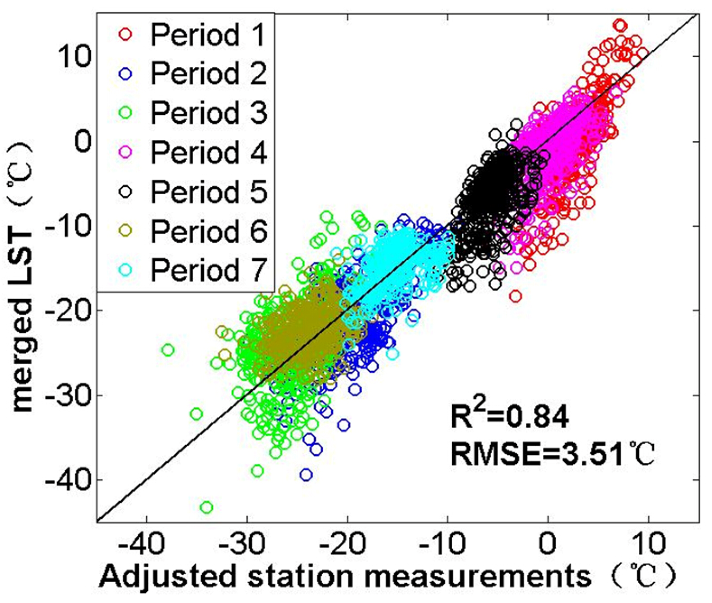
4.4. Validation of Merged LSTs with the Adjusted Station Measurements

Because no 0 cm LST data were available in this area, errors were likely introduced when using the 0–5 cm soil temperatures to validate the merged LSTs. To solve this problem, we established an empirical relationship between soil temperatures and LSTs by comparing the station temperatures and corresponding MODIS temperatures under clear-sky conditions from 1 August 2010 to 28 July 2011. MODIS temperatures were used for three reasons: first, MODIS LST is considered as hard data in the merging process and has also been used to validate the AMSR-E LST in the production process. Second, more than 90% of the study area is covered by grasses, so the MODIS LSTs under clear-sky conditions could yield relatively accurate values in this homogeneous area. Third, a total of 6290 data pairs were used in the statistics, and the RANSAC method [54] was utilized to eliminate the outliers to obtain the best regression line. As shown in Figure 8, the correlation coefficient between them is 0.933, and R 2 = 0.87 , which demonstrates that the relationship between 0–5 cm soil temperatures and LSTs is robust. The equation for the relationship is as follows:
LST = 1.245 T 0 ~ 5   cm 8.686
where T 0 ~ 5   cm is the temperature at a soil depth of 0–5 cm. Equation (9) was used to adjust the station measurements before the validation.
Figure 8. Comparison of station measurements (0–5 cm soil temperatures) with the corresponding MODIS LSTs under clear-sky conditions for the period from 1 August 2010 to 28 July 2011.
Remotesensing 08 00105 g008
Finally, station measurements at a soil depth of 0–5 cm were adjusted with Equation (9) and then used to validate the merged LST. The result is shown in Figure 9. After the adjustment process, the merged LSTs fit the adjusted station measurements well. The correlation coefficient between them is 0.917, with R 2 = 0.84 and an RMSE of the seven periods of 3.51 °C. In contrast, correlations and RMSEs between the adjusted station measurements and MODIS LST or AMSR-E LST were also calculated, with R 2 values of 0.85 and 0.62, and RMSE values of 3.23 and 5.78, respectively.
To examine how the accuracy of merged LST varies with the amount of data used in the BME estimation procedure, the RMSEs for the seven periods with different availabilities were calculated, as shown in Table 5. The RMSEs of merged LSTs generally declined with an increasing amount of data. In period 7, the availability of the MODIS LSTs was 91.4%, and the RMSE of merged LSTs was 2.31 °C, which approaches the accuracy of the MODIS LSTs. In period 1, when the availability of the MODIS LSTs was only 25.2%, the RMSE of the merged LSTs was 4.53 °C, which is similar to the accuracy of the AMSR-E LSTs.
Figure 9. Comparison of the adjusted station measurements with the corresponding merged LSTs for different periods (from period 1 to 7).
Remotesensing 08 00105 g009
Table 5. Validation of the merged LSTs for each period.
PeriodPeriod 1Period 2Period 3Period 4Period 5Period 6Period 7
Availability of MODIS LSTs25.2%32.4%47.5%57.6%73.7%83.6%91.4%
Availability of AMSR-E LSTs76.3%87.5%86.3%95.6%85.6%85.0%95.0%
RMSE4.53 °C4.07 °C4.26 °C3.56 °C3.10 °C3.08 °C2.31 °C

4.5. Comparison of the Differences between BME Merged LSTs and Mixed LSTs

LSTs selected on 17 November 2010 (period 7) for MODIS LST, AMSR-E LST, merged LST by the BME method, and mixed LST by the gap filling method are shown in Figure 10a–d, respectively. As can be concluded from Figure 10, compared with the mixed LSTs by the gap filling method, the merged LSTs by the BME method have some advantages. As observed in the red circle frames in Figure 10, the merged LSTs exhibit higher spatial continuity than the mixed LSTs. In addition, it could be inferred that the accuracy of the merged LSTs in the MODIS blank area basically falls between the accuracy of the MODIS LSTs and AMSR-E LSTs, whereas the accuracy of the mixed LSTs was completely determined by the quality of the AMSR-E LSTs. Finally, because the merged LSTs were estimated by the probability distribution characteristics of variability in the random field, in the blank area where both the AMSR-E LSTs and MODIS LSTs are missing, the LSTs could still be estimated by the BME method. In contrast, in the same situation, the LSTs could not be obtained by the gap filling method.
Figure 10. Comparison of the LSTs (in Kelvin): (a) MODIS LST; (b) AMSR-E LST; (c) merged LST by the BME method; and (d) mixed LST by the gap filling method on 17 November 2010.
Remotesensing 08 00105 g010

5. Discussion

The LSTs derived from TIR remote sensors usually display high accuracy, but they are incomplete. In contrast, the LSTs retrieved from PMW remote sensors are nearly complete but display low accuracy and coarse spatial resolution. Both the incompleteness problem of TIR data and the low accuracy and coarse spatial resolution problem of PMW data have limited the applications of LST products in climatological and surface energy balance studies. To solve these problems, it is possible to use their respective advantages to produce more complete and accurate LST products. In this paper, the BME method was used to blend the satellite LST products retrieved from TIR (MODIS) and PMW (AMSR-E) remote sensing data. In this method, the error model proposed by Li et al. [46] was used to link the LST values at different spatial resolutions to generate soft data, and the residuals de-trended from MODIS LSTs were used to model the covariance functions. After the merging process, the estimated LSTs were spatiotemporally continuous with an availability of 100%. Because LSTs are different from 0–5 cm soil temperatures, before validating the merged LSTs, the station measurements were adjusted with Equation (9). The validation showed that the merged LST has a strong correlation (r = 0.90) with the adjusted station measurements, with an RMSE of 3.51 °C. Furthermore, the merged LSTs by the BME method were also compared with the mixed LSTs by the gap filling method. The results showed that the merged LSTs have the following advantages: (1) better spatial continuity and (2) higher accuracy.
In addition, to analyze how the accuracy of merged LST varies with the amount of data used in the estimated procedure, seven periods of data were selected according to the availability of MODIS LSTs, with an availability range of 25.2% to 91.4%. After the blending process with the BME method, the merged LSTs were validated with the adjusted station measurements. The results showed that the RMSEs for the merged LSTs decreased with increasing amount of utilized data, with a range of 2.31 °C to 4.53 °C, which was close to the accuracies of the MODIS LSTs and AMSR-E LSTs, respectively. This can be attributed to the fact that a lower amount of data reduces the ability of capturing accurate temporal-spatial LST trends, which finally influences the estimation procedure. As seen in the covariance modeling process, the covariance of periods 1 and 2 presented fluctuation characteristics due to the low availabilities of 25.2% and 32.4%, and the final RMSEs for the merged LSTs in period 1 and 2 are only 4.53 and 4.07, respectively.
One point that should be noted is that errors may be introduced when using MODIS LST to replace the 0 cm LST measurements to establish the relationship between LSTs and 0–5 cm soil temperatures. Another factor that may influence the result is that the sampling depth of LSTs retrieved from PMW data is different from that of MODIS. For the TIR band, the thermal sampling depth is approximately 0 cm, but for the PMW band, this depth is influenced by the surface moisture, frequency, and other factors. Thus, the merged LST has a different sampling depth error.
Through this study, it has been demonstrated that the method was applicable to night-time LST. The results show that the accuracy of merged LSTs increases with the increasing quantity of data. The accuracy was generally lower than that of the MODIS LSTs and higher than that of the AMSR-E LSTs. As the soft data component in the BME method, the accuracy of the AMSR-E LSTs may influence the accuracy of the merged LSTs, especially when MODIS LST data are missing. The accuracy of the AMSR-E daily LSTs varies according to land cover type, time of day, and season [32]. Therefore, it can be concluded that the accuracy and spatial-temporal variability of merged LSTs are also influenced by the land-cover type, time, and season. This is worthy of further exploration.

6. Conclusions

In this study, the BME method was introduced to merge 1 km grid land surface temperature (LST) from the 1 km grid MODIS thermal infrared LST product (channels 11 and 12 microns) and the 25 km grid AMSR-E LST product. The method was validated in the central Tibetan Plateau around Naqu City, an area of approximately 100 2  km 2 , against 0–5 cm in situ surface temperature measurements and over seven time periods selected corresponding to the availability of MODIS/AMSR-E data over a period spanning from 1 August 2010 to 28 July 2011. The results showed that the merged LST has 100% pixel availability and an RMSE of 3.51 °C.
In summary, it is practical to use the BME approach to blend night-time LSTs retrieved from MODIS and AMSR-E data to produce spatiotemporally complete LSTs. Compared to the simple gap filling method, the merged LST by BME method has better spatial continuity and better spatial correlation with elevation level maps. Even when both MODIS LSTs and AMSR-E LSTs are missing, the LST could still be estimated by the BME method. The estimation accuracy of merged LSTs were influenced by the quality and quantity of data used in the merging process. A sufficient amount of data was required to obtain an accurate spatiotemporal random field of the variables, which may result in fusion products with high precision. Moreover, different sampling depths between PMW and TIR data may affect the fusion performance and require further studies. In this paper, we merely integrated LSTs from two different remote sensors. In fact, BME has the potential to fuse field measurements and remotely sensed data; however, further examination is still needed to verify its efficiency.

Acknowledgments

This study was supported by the National Basic Research Program of China (No. 2013CB733406 and No. 2013CB733403) and the National Natural Science Foundation of China (No. 41171260).

Author Contributions

Lingmei Jiang and Xiaokang Kou designed the work and wrote the manuscript. Shuang Yan modified the format of the paper. Yanchen Bo and Linna Chai gave useful suggestions.

Conflicts of Interest

The authors declare no conflict of interest.

References

  1. Prihodko, L.; Goward, S.N. Estimation of air temperature from remotely sensed surface observations. Remote Sens. Environ. 1997, 60, 335–346. [Google Scholar] [CrossRef]
  2. Solomon, S.; Qin, D.; Manning, M.; Chen, Z.; Marquis, M.; Averyt, K.B.; Tignor, M.; Miller, H.L. Climate Change 2007: The Physical Science Basis; Cambridge University Press: Cambridge, UK; New York, NY, USA, 2007; Volume 6. [Google Scholar]
  3. Vogt, J.V.; Viau, A.A.; Paquet, F. Mapping regional air temperature fields using satellite-derived surface skin temperatures. Int. J. Climatol. 1997, 17, 1559–1579. [Google Scholar] [CrossRef]
  4. Jia, Y.Y.; Li, Z.L. Progress in land surface temperature retrieval from passive microwave remotely sensed data. Prog. Geogr. 2006, 25, 96–105. [Google Scholar]
  5. Zhou, J.; Chen, Y.H.; Wang, J.F.; Zhan, W.F. Maximum nighttime urban heat island (UHI) intensity simulation by integrating remotely sensed data and meteorological observations. IEEE J. Sel. Top. Appl. Earth Observ. 2011, 4, 138–146. [Google Scholar] [CrossRef]
  6. Marquı́nez, J.; Lastra, J.; Garcı́a, P. Estimation models for precipitation in mountainous regions: The use of GIS and multivariate analysis. J. Hydrol. 2003, 270, 1–11. [Google Scholar] [CrossRef]
  7. Li, Z.L.; Tang, B.H.; Wu, H.; Ren, H.Z.; Yan, G.J.; Wan, Z.M.; Trigo, I.F.; Sobrino, J.A. Satellite-derived land surface temperature: Current status and perspectives. Remote Sens. Environ. 2013, 131, 14–37. [Google Scholar] [CrossRef]
  8. Lakshmi, V.; Czajkowski, K.; Dubayah, R.; Susskind, J. Land surface air temperature mapping using TOVS and AVHRR. Int. J. Remote Sens. 2001, 22, 643–662. [Google Scholar] [CrossRef]
  9. Aumann, H.H.; Chahine, M.T.; Gautier, C.; Goldberg, M.D.; Kalnay, E.; McMillin, L.M.; Revercomb, H.; Rosenkranz, P.W.; Smith, W.L.; Staelin, D.H.; et al. AIRS/AMSU/HSB on the Aqua mission: Design, science objectives, data products, and processing systems. IEEE Trans. Geosci. Remote Sens. 2003, 41, 253–264. [Google Scholar] [CrossRef]
  10. Zhou, J.; Li, J.; Zhang, L.X. Intercomparison of methods for estimating land surface temperature from a Landsat-5 TM image in an arid region with low water vapour in the atmosphere. Int. J. Remote Sens. 2012, 33, 2582–2602. [Google Scholar] [CrossRef]
  11. Stisen, S.; Sandholt, I.; Nørgaard, A.; Fensholt, R.; Eklundh, L. Estimation of diurnal air temperature using MSG SEVIRI data in West Africa. Remote Sens. Environ. 2007, 110, 262–274. [Google Scholar] [CrossRef]
  12. Vancutsem, C.; Ceccato, P.; Dinku, T.; Connor, S.J. Evaluation of MODIS land surface temperature data to estimate air temperature in different ecosystems over Africa. Remote Sens. Environ. 2010, 114, 449–465. [Google Scholar] [CrossRef]
  13. Jang, J.D.; Viau, A.A.; Anctil, F. Neural network estimation of air temperatures from AVHRR data. Int. J. Remote Sens. 2004, 25, 4541–4554. [Google Scholar] [CrossRef]
  14. Guo, Z.; Chen, Y.; Cheng, M.; Jiang, H. Near-surface air temperature retrieval from Chinese Geostationary FengYun Meteorological Satellite (FY-2C) data. Int. J. Remote Sens. 2014, 35, 3892–3914. [Google Scholar] [CrossRef]
  15. Dash, P.; Göttsche, F.M.; Olesen, F.S.; Fischer, H. Land surface temperature and emissivity estimation from passive sensor data: Theory and practice—Current trends. Int. J. Remote Sens. 2002, 23, 2563–2594. [Google Scholar] [CrossRef]
  16. Wan, Z.M.; Dozier, J. A generalized split-window algorithm for retrieving land-surface temperature from space. IEEE Trans. Geosci. Remote Sens. 1996, 34, 892–905. [Google Scholar]
  17. Gillespie, A.T.; Rokugawa, S.; Hook, S. Temperature emissivity separation from Advanced Spaceborne Thermal Emission and Reflection Radiometer (ASTER) images. IEEE Trans. Geosci. Remote Sens. 1998, 36, 1113–1126. [Google Scholar] [CrossRef]
  18. Qin, Z.; Karnieli, A.; Berliner, P. A mono-window algorithm for retrieving land surface temperature from Landsat TM data and its application to the Israel–Egypt border region. Int. J. Remote Sens. 2001, 22, 3719–3746. [Google Scholar] [CrossRef]
  19. Zhou, J.; Li, J.; Zhao, X.; Zhan, W.F.; Guo, J.X. A modified single channel algorithm for land surface temperature retrieval from HJ-1B satellite data. J. Infrared Millim. Waves 2011, 30, 61–67. [Google Scholar] [CrossRef]
  20. Becker, F.; Li, Z.L. Towards a local split window method over land surfaces. Int. J. Remote Sens. 1990, 11, 369–393. [Google Scholar] [CrossRef]
  21. Owe, M.; Van de Griend, A.A. On the relationship between thermodynamic surface temperature and high-frequency (37 GHz) vertically polarized bright-ness temperature under semi-arid conditions. Int. J. Remote Sens. 2001, 22, 3521–3532. [Google Scholar] [CrossRef]
  22. Mcfarland, M.J.; Miller, R.L.; Neale, C.M.U. Land surface temperature derived from the SSM/I passive microwave brightness temperatures. IEEE Trans. Geosci. Remote Sens. 1990, 28, 839–845. [Google Scholar] [CrossRef]
  23. Holmes, T.R.H.; de Jeu, R.A.M.; Owe, M.; Dolman, A.J. Land surface temperature from Ka band (37 GHz) passive microwave observations. J. Geophys. Res. 2009, 114. [Google Scholar] [CrossRef]
  24. Royer, A.; Poirier, S. Surface temperature spatial and temporal variations in North America from homogenized satellite SMMR-SSM/I microwave measurements and reanalysis for 1979–2008. J. Geophys. Res. 2010, 115. [Google Scholar] [CrossRef]
  25. Surdyk, S. Using microwave brightness temperature to detect short-term surface air temperature changes in Antarctica: An analytical approach. Remote Sens. Environ. 2002, 80, 256–271. [Google Scholar] [CrossRef]
  26. Basist, A.; Grody, N.C.; Peterson, T.C. Using the Special Sensor Microwave/Imager to monitor land surface temperatures, wetness, and snow cover. J. Appl. Meteorol. 1998, 37, 888–911. [Google Scholar] [CrossRef]
  27. Seemann, S.W.; Borbas, E.E.; Li, J.; Menzel, W.P.; Gumley, L.E. MODIS Atmospheric Profile Retrieval Algorithm Theoretical Basis Document; NASA: Greenbelt, MD, USA, 2006. [Google Scholar]
  28. Jones, L.A.; Ferguson, C.R.; Kimball, J.S.; Zhang, K.; Chan, S.T.K.; McDonald, K.C.; Njoku, E.G.; Wood, E.F. Satellite microwave remote sensing of daily land surface air temperature minima and maxima from AMSR-E. IEEE J. Sel. Top. Appl. Earth Obser. Remote Sens. 2010, 3, 111–123. [Google Scholar] [CrossRef]
  29. Chen, S.S.; Chen, X.Z.; Chen, W.Q. A simple retrieval method of land surface temperature from AMSR-E passive microwave data—A case study over Southern China during the strong snow disaster of 2008. Int. J. Appl. Earth Observ. Geoinf. 2011, 13, 140–151. [Google Scholar] [CrossRef]
  30. Bisht, G.; Venturini, V.; Islam, S.; Jiang, L. Estimation of the net radiation using MODIS (moderate resolution imaging spectroradiometer) data for clear sky days. Remote Sens. Environ. 2005, 97, 52–67. [Google Scholar] [CrossRef]
  31. Batra, N.; Islam, S.; Venturini, V.; Bisht, G.; Jiang, L. Estimation and comparison of evapotranspiration from MODIS and AVHRR sensors for clear sky days over the Southern Great Plains. Remote Sens. Environ. 2006, 103, 1–15. [Google Scholar] [CrossRef]
  32. Zhou, J.; Dai, F.; Zhang, X.; Zhao, S.; Li, M. Developing a temporally land cover-based look-up table (TL-LUT) method for estimating land surface temperature based on AMSR-E data over the Chinese landmass. Int. J. Appl. Earth Observ. Geoinf. 2015, 34, 35–50. [Google Scholar] [CrossRef]
  33. Hachem, S.; Allard, M.; Duguay, C. Using the MODIS land surface temperature product for mapping permafrost: An application to Northern Quebec and Labrador, Canada. Permafr. Periglac. Processes 2009, 20, 407–416. [Google Scholar] [CrossRef]
  34. Ran, Y.H.; Li, X.; Jin, R. Estimation of the mean annual surface temperature and surface frost number using the MODIS land surface temperature products for mapping permafrost in China. In Proceedings of the Tenth International Conference on Permafrost (TICOP), Salekhard, Russia, 25–29 June 2012; pp. 317–321.
  35. Ryu, Y.; Baldocchi, D.D.; Kobayashi, H.; Ingen, C.; Li, J.; Black, T.A.; Beringer, J.; Gorsel, E.; Knohl, A.; Law, B.E. Integration of MODIS land and atmosphere products with a coupled process model to estimate gross primary productivity and evapotranspiration from 1 km to global scales. Glob. Biogeochem. Cycle 2011, 25, GB4017. [Google Scholar] [CrossRef]
  36. Bisht, G.; Bras, R.L. Estimation of net radiation from the MODIS data under all sky conditions: Southern Great Plains case study. Remote Sens. Environ. 2010, 114, 1522–1534. [Google Scholar] [CrossRef]
  37. Jang, K.; Kang, S.; Lim, Y.; Jeong, S.; Kim, J.; Kimball, J.S.; Hong, S.Y. Monitoring daily evapotranspiration in Northeast Asia using MODIS and a regional Land Data Assimilation System. J. Geophys. Res. Atmos. 2013, 118, 927–940. [Google Scholar] [CrossRef]
  38. Jang, K.; Kang, S.; Kimball, J.S.; Hong, S.Y. Retrievals of all-weather daily air temperature using MODIS and AMSR-E data. Remote Sens. 2014, 6, 8387–8404. [Google Scholar] [CrossRef]
  39. Christakos, G. Modern Spatiotemporal Geostatistics; Oxford University Press: New York, NY, USA, 2000. [Google Scholar]
  40. Christakos, G.; Serre, M.L. BME analysis of spatiotemporal particulate matter distributions in North Carolina. Atmos. Environ. 2000, 34, 3393–3406. [Google Scholar] [CrossRef]
  41. Bogaert, P.; Christakos, G.; Jerrett, M.; Yu, H.L. Spatiotemporal modelling of ozone distribution in the State of California. Atmos. Environ. 2009, 43, 2471–2480. [Google Scholar] [CrossRef]
  42. Christakos, G.; Kolovos, A.; Serre, M.L.; Vukovich, F. Total ozone mapping by integrating databases from remote sensing instruments and empirical models. IEEE Trans. Geosci. Remote Sens. 2004, 42, 991–1008. [Google Scholar] [CrossRef]
  43. D’Or, D.; Bogaert, P.; Christakos, G. Application of the BME approach to soil texture mapping. Stoch. Environ. Res. Risk Assess. 2001, 15, 87–100. [Google Scholar] [CrossRef]
  44. Douaik, A.; van Meirvenne, M.; Tóth, T. Statistical methods for evaluating soil salinity spatial and temporal variability. Soil Sci. Soc. Am. J. 2007, 71, 1629–1635. [Google Scholar] [CrossRef]
  45. Lee, S.J.; Balling, R.; Gober, P. Bayesian maximum entropy mapping and the soft data problem in urban climate research. Ann. Assoc. Am. Geogr. 2008, 98, 309–322. [Google Scholar] [CrossRef]
  46. Li, A.; Bo, Y.; Zhu, Y.; Guo, P.; Bi, J.; He, Y. Blending multi-resolution satellite sea surface temperature (SST) products using Bayesian maximum entropy method. Remote Sens. Environ. 2013, 135, 52–63. [Google Scholar] [CrossRef]
  47. Wu, G.; Liu, Y.; Zhang, Q.; Duan, A.; Wang, T.; Wan, R.; Liu, X.; Li, W.; Wang, Z.; Liang, X. The influence of mechanical and thermal forcing by the Tibetan Plateau on Asian climate. J. Hydrometeorol. 2007, 8, 770–789. [Google Scholar] [CrossRef]
  48. Yang, K.; Guo, X.; He, J.; Qin, J.; Koike, T. On the climatology and trend of the atmospheric heat source over the Tibetan Plateau: An experiments-supported revisit. J. Clim. 2011, 24, 1525–1541. [Google Scholar] [CrossRef]
  49. Wan, Z. New refinements and validation of the MODIS land-surface temperature/emissivity products. Remote Sens. Environ. 2008, 112, 59–74. [Google Scholar] [CrossRef]
  50. Yang, K.; Qin, J.; Zhao, L.; Chen, Y.Y.; Tang, W.; Han, M.; Chen, Z.; Lv, N.; Ding, B.; Wu, H.; et al. A multi-scale soil moisture and freeze-thaw monitoring network on the third pole. Bull. Am. Meteorol. Soc. 2013, 94, 1907–1916. [Google Scholar] [CrossRef]
  51. Christakos, G. Random Field Models in Earth Sciences; Academic Press: San Diego, CA, USA, 1992. [Google Scholar]
  52. Spadavecchia, L.; Williams, M. Can spatio-temporal geostatistical methods improve high resolution regionalisation of meteorological variables? Agric. For. Meteorol. 2009, 149, 1105–1117. [Google Scholar] [CrossRef]
  53. Olea, R.A. Normalization. In Geostatistics for Engineers and Earth Scientists; Springer Science+Business Media: New York, NY, USA, 1999; pp. 31–38. [Google Scholar]
  54. Bolles, R.C.; Fischler, M.A. A RANSAC-based approach to model fitting and its application to finding cylinders in range data. IJCAI 1981, 1981, 637–643. [Google Scholar]

