Article

Potential of Resolution-Enhanced Hyperspectral Data for Mineral Mapping Using Simulated EnMAP and Sentinel-2 Images

1
Department of Advanced Interdisciplinary Studies, University of Tokyo, 4-6-1 Komaba, Meguro-ku, Tokyo 153-8904, Japan
2
Department of Electronics and Informatics, Vrije Universiteit Brussel, Pleinlaan 2, Brussels 1050, Belgium
3
Helmholtz Center Potsdam, GFZ German Research Center for Geosciences, Remote Sensing Section, Telegrafenberg A17, Potsdam 14473, Germany
*
Author to whom correspondence should be addressed.
Submission received: 11 December 2015 / Revised: 22 January 2016 / Accepted: 17 February 2016 / Published: 24 February 2016

Abstract

:
Spaceborne hyperspectral images are useful for large scale mineral mapping. Acquired at a ground sampling distance (GSD) of 30 m, the Environmental Mapping and Analysis Program (EnMAP) will be capable of putting many issues related to environment monitoring and resource exploration in perspective with measurements in the spectral range between 420 and 2450 nm. However, a higher spatial resolution is preferable for many applications. This paper investigates the potential of fusion-based resolution enhancement of hyperspectral data for mineral mapping. A pair of EnMAP and Sentinel-2 images is generated from a HyMap scene over a mining area. The simulation is based on well-established sensor end-to-end simulation tools. The EnMAP image is fused with Sentinel-2 10-m-GSD bands using a matrix factorization method to obtain resolution-enhanced EnMAP data at a 10 m GSD. Quality assessments of the enhanced data are conducted using quantitative measures and continuum removal and both show that high spectral and spatial fidelity are maintained. Finally, the results of spectral unmixing are compared with those expected from high-resolution hyperspectral data at a 10 m GSD. The comparison demonstrates high resemblance and shows the great potential of the resolution enhancement method for EnMAP type data in mineral mapping.

Graphical Abstract

1. Introduction

Hyperspectral images provide important information for the characterization of lithology. Using hundreds of contiguous spectral bands with a narrow bandwidth, a pixel spectrum is generated for the potential discrimination of target minerals [1,2]. Spectral unmixing is an important technique for discerning minerals at a subpixel scale using hyperspectral image data. Geological mapping and mineral exploration with hyperspectral images have been studied for decades [3,4,5]. In particular, the shortwave infrared (SWIR) spectral range of 2.0–2.5 µm is considered to have the most important diagnostic absorption features, which are related to the vibration processes in atomic bonds. Numerous distinctive minerals associated with primary lithologies and with various alteration styles can be identified; for instance, Al–OH at 2.2 µm, Mg–OH at 2.3 µm, and Ca–CO3 at 2.32–2.35 µm [6].
Most geological applications using hyperspectral remote sensing, including mineral explorations, have relied on airborne acquisition to obtain high-spatial-resolution data. However, the airborne acquisition of hyperspectral images with high spatial resolution can become overly expensive when the coverage is very large. The spaceborne Environmental Mapping and Analysis Program (EnMAP) is dedicated to environmental applications of state-of-the-art hyperspectral technology (www.enmap.org) [7]. The launch of EnMAP is planned for mid-2018 and the expected mission lifetime is five years. A major objective of EnMAP is the monitoring and exploration of natural resources. Its fine spectral resolution of 6.5 nm in the visible and near infrared (VNIR) range (420–1000 nm) and 10 nm in the SWIR range (900–2450 nm) will make it well suited for geological mapping. It will have a swath width of 30 km and 242 spectral bands at 0.4–2.5 µm. This will be a great improvement on the 7 km swath width of the concurrent Hyperion [8]. EnMAP has a 27-day revisit cycle (off-nadir four days) and is able to acquire an along-track length of 5000 km per day based on the acquisition requests of users. Even equipped with the latest technology, a compromise must be made between scientific ambition and practicality regarding the spatial resolution. Therefore, EnMAP images will be acquired at a ground sampling distance (GSD) of 30 m. This spatial resolution will unfortunately limit the applicability of such data to a certain extent.
Owing to the high potential of spaceborne hyperspectral images in many applications, researchers are keen to look into possibilities for enhancing the spatial resolution. Some have studied superresolution image reconstruction using temporal and angular images [9,10]. The challenges in such approaches are the availability of quality temporal images and the complex manipulation of big data with high dimensionality. Changes in surface cover that occur between acquisitions can also have negative effects on the operation. Recent developments in image fusion have motivated new exploration of the spatial resolution enhancement of hyperspectral images [11,12]. Pansharpening, a traditional method applied to multispectral images, has received increasing attention for its use with hyperspectral images [13,14]. Its popularity can be attributed to the convenience of obtaining high-resolution multispectral images in the VNIR spectral range by a conventional method. The expected increasing demand for high-resolution hyperspectral images in the future has encouraged more studies, and recently newer resolution enhancement approaches based on hyperspectral and multispectral image fusion have shown highly promising results [15,16,17,18,19,20,21,22,23,24].
Sentinel-2 will provide high-resolution multispectral data with a short revisiting time (every 5 days with two satellites). The mission will acquire 13 bands in the VNIR and SWIR ranges with various spatial resolutions (10, 20 and 60 m), which contribute to a wide range of application including mineral mapping [25]. Table 1 lists the band descriptions. For experiments on resolution enhancement with hyperspectral EnMAP data, Sentinel-2 data is a very good option for obtaining the required high-resolution images. Even though changes between acquisitions still could occur, the 5-day revisiting time means there is a higher probability of avoiding such changes and it is easier to obtain high-resolution VNIR images at a similar time to hyperspectral acquisition.
A key limitation of previous studies on hyperspectral and multispectral image fusion is that fused images are validated mainly by quantitative measures of image quality but studies on its impact on applications are still lacking. An accurate validation of the fusion process on a pixel level can be performed only within a simulation study, because in such case the optimum result is known. Many of the conventional simulation studies consider mainly the image generation process with spectral response functions (SRFs), point spread functions (PSFs) and noise for simulation. However, a more realistic simulation should takes into account the entire image acquisition and processing chain because the characteristics of real data are influenced by instrumental and environmental parameters that naturally also impact the quality of the fused data products.
In this study, a simulated EnMAP-Sentinel image set forms the basis to investigate whether spatially enhanced hyperspectral data obtained from the fusion of hyperspectral and multispectral images can retain spectral fidelity and consequently contribute to mineral mapping. Sensor end-to-end simulation tools [26,27,28,29] that consider the entire image acquisition and processing chains are used for simulating realistic EnMAP and Sentinel-2 images. We demonstrate the fusion of simulated EnMAP and Sentinel-2 VNIR images using various methods (one matrix factorization method and two pansharpening methods) and validate the quality of the fused data products in regard to the preservation of the original spectral information content. Among the hyperspectral and multispectral image fusion methods, we have focused on a matrix factorization method that requires relative sensor configurations, such as SRFs and PSFs, but produces good results with only a moderate computational burden [14]. Our contribution is threefold: we present (1) a validation of hyperspectral image enhancement by continuum removal and spectral unmixing in terms of its applicability in mineral mapping; (2) image fusion using sensor end-to-end simulation data; (3) hyperspectral and multispectral image fusion without the overlap of SRFs.

2. Hyperspectral and Multispectral Image Fusion

2.1. Related Work

Hyperspectral and multispectral image fusion enables the production of higher-spatial-resolution hyperspectral imagery while preserving high spectral accuracy, making it advantageous over pansharpening. The fusion problem is formulated as an ill-posed inverse problem. Hyperspectral and multispectral image fusion is still an open issue, and the methods presented in the literature for tackling this issue are limited in number compared to those proposed for pansharpening.
A wavelet-based technique that inherited the pansharpening algorithm was first proposed for hyperspectral and multispectral image fusion [30,31]. However, its performance strongly depended on the spectral sampling method, making it difficult to enhance the spatial resolution of all hyperspectral band images.
A Bayesian method based on a maximum a posteriori (MAP) estimation was a major breakthrough in terms of the capability to enhance the spatial resolution of all hyperspectral band images using higher-spatial-resolution data acquired by a panchromatic or multispectral imager [15,16]. This method adopted a stochastic mixing model (SMM) to estimate the underlying spectral scene characteristics and integrated them into a MAP-based fusion framework. The optimization was performed in the principal component domain rather than the spectral domain to decrease the computational burden. The MAP/SMM method outperformed those based on conventional pansharpening algorithms and has been further extended using wavelet transforms to improve noise resistance [17].
Methods based on a matrix factorization or spectral unmixing perspective have been attracting attention in recent years owing to their straightforward interpretation of the fusion process and state-of-the-art performance [18,19,20]. Coupled nonnegative matrix factorization (CNMF) formulates the image fusion problem as a coupled spectral unmixing problem [18]. A high-spectral-resolution endmember matrix and high-spatial-resolution abundance matrix are obtained from hyperspectral and multispectral images, respectively, by coupled spectral unmixing. The fused image can be reconstructed by the multiplication of the two underlying matrices. Sparse regularization on the abundance fractions or local image processing was shown to be effective for mitigating the ill-posedness of the inverse problem and improving the quality of fusion products [19,20].
When the two underlying matrices of the fused image are generalized as the subspace transform matrix and the representation coefficient matrix, the fusion problem is formulated within the Bayesian fusion model, which includes the MAP/SMM method. Recent advances in this approach can be characterized as the use of regularization in the problem by defining an appropriate prior distribution for the observed scene, such as patch-based sparse representation and vector-total-variation-based regularization of the spatial distribution of subspace coefficients [21,22].
Pansharpening methods can be applied to hyperspectral and multispectral image fusion by regarding each multispectral band and spectrally corresponding hyperspectral bands as panchromatic and multispectral images, respectively, in the conventional pansharpening framework. A generalization of pansharpening that can be adapted to hyperspectral and multispectral image fusion has recently been studied [23]. One of the state-of-the-art pansharpening methods based on patch-based sparse representation was successfully extended to solve the fusion problem [24]. Major challenges for pansharpening-based methods are the discontinuity of spectra in the fused image and the fusion of spectrally non-overlapping images.
Many recent methods are summarized in a recently published review paper of hyperspectral pansharpening [14], which can be seen as a particular case of hyperspectral and multispectral image fusion. In this paper, we focus on CNMF owing to its straightforward interpretation, robust performance as a benchmark method as shown in the literature, and its applicability to the fusion of spectrally non-overlapping images, which will be tackled in this paper.

2.2. The CNMF Algorithm

Hyperspectral and multispectral image fusion aims to estimate a high-spatial-resolution hyperspectral image ( X L × P ) by fusing a low-spatial-resolution hyperspectral image ( Y h L × P h ) and a high-spatial-resolution multispectral image ( Y m L m × P ). L and L m denote the numbers of spectral bands of the hyperspectral and multispectral sensors, respectively. P h and P denote the numbers of pixels in the hyperspectral and multispectral images, respectively. L > L m and P h < P are satisfied by considering the trade-off between the spectral and spatial resolutions of the two sensors.
CNMF aims to reconstruct high-spatial-resolution hyperspectral data by extracting the underlying spectral scene characteristics at a high spatial resolution via matrix factorization, which can be interpreted as spectral unmixing. Spectral unmixing of the hyperspectral image provides the spectral signatures of endmembers and a set of fractional abundances for each pixel at a large GSD. The multispectral image itself cannot achieve accurate spectral unmixing due to broader SRFs at limited wavelength ranges; however, it is helpful to determine the detailed spatial distribution of abundances at a smaller GSD once the spectral signatures and the fractional abundances are obtained for each pixel at a large GSD by spectral unmixing of the hyperspectral image. The multiplication of the spectral signatures and their high-resolution abundance maps leads to the reconstruction of high-spatial-resolution hyperspectral data.
We assume that the two observed images are acquired over the same area under the same atmospheric and illumination conditions and are geometrically coregistered. The low-spatial-resolution hyperspectral image and the multispectral image can be viewed as degraded versions of the target image in the spatial and spectral domains, respectively. Therefore, Y h and Y m are modeled as
Y h = XBS + N h
Y m = RX + N m
Here, B P × P is a matrix modeling the PSF of the hyperspectral sensor, S P × P h is the spatial downsampling matrix and R L m × L is the spectral transform matrix, with its columns representing the spectral responses of the multispectral sensor. N h and N m are the residuals. The relative sensor characteristics, such as B and R, can be estimated from the observed data sources when they are not given as prior knowledge [32].
The unmixing-based approaches to fusion introduce linear mixture models for hyperspectral images. Linear spectral mixture models are commonly used for spectral unmixing owing to their physical effectiveness and mathematical simplicity [33]. The spectrum at each pixel is assumed to be a linear combination of several endmember spectra. Therefore, X is formulated as
X = EA + N
where E L × M is the spectral signature matrix, with the column vectors corresponding to the M endmember spectra, A M × P is the abundance matrix, with each column vector denoting the abundance fractions of all the endmembers at the pixel, and N is the residual. The endmember spectra and abundance fractions are nonnegative. By substituting Equation (3) into Equations (1) and (2), Y h and Y m can be approximated as
Y h E A h
Y m E m A
where we define the spatially degraded abundance matrix A h M × P h and the spectrally degraded endmember matrix E m L m × M as
A h = ABS
E m = RE
CNMF focuses on the estimation of the spectral signatures of endmembers (E) and the corresponding high-resolution abundance maps (A) by the coupled spectral unmixing of the low-spatial-resolution hyperspectral image ( Y h ) and the high-spatial-resolution multispectral image ( Y m ). CNMF alternately unmixes Y h and Y m in the framework of nonnegative matrix factorization (NMF) [34,35] to estimate E and A under the constraints of the relative sensor characteristics given by Equations (6) and (7). NMF decomposes a nonnegative data matrix into a product of two nonnegative matrices, and it has been shown to be effective for spectral unmixing satisfying physical constraints without assuming the presence of pure pixels. The squared Frobenius norm of a residual matrix in a linear spectral mixture model is commonly used for a cost function. NMF unavoidably converges to local minima depending on the initialization. CNMF alternately takes advantage of the two images, i.e., the spectral resolution of the hyperspectral image and the spatial resolution of the multispectral image, to initialize the other spectral unmixing so that the optimization can converge to a better local minimum.
CNMF starts with NMF unmixing of the low-spatial-resolution hyperspectral image. The matrix E can be initialized using endmember extraction methods, for example, vertex component analysis (VCA) [36]. In this work, since our interest is focused on the SWIR range of fused data, this endmember extraction process is carried out using only SWIR bands. E and A h are then alternately optimized by Lee and Seung’s multiplicative update rules [35]. Next, A is estimated from the multispectral image. E m is set by Equation (7) and A is initialized by the spatially up-sampled matrix of A h obtained by bilinear interpolation. The sequential unmixing for the hyperspectral image is performed after initializing A h by Equation (6). After that, the two images are alternately unmixed until convergence. Finally, the target image is obtained by the multiplication of E and A. More details of the implementation are given in [18].

3. Materials and Validation Methods

3.1. Study Area and Data Preparation

An airborne HyMap scene of Rodalquilar in the south-eastern corner of Spain was used to generate EnMAP and Sentinel-2 Level-2a data products. The airborne image covers the Sierra del Cabo de Gata (Cabo de Gata National Park), where a gold mining area is situated that has been used in several studies [6,37]. Volcanic rocks have undergone a transformation to minerals such as silica, alunite, kaolinite, montmorillonite and chlorite. Various alteration phases can be distinguished, and gold deposits have been found in the central part of the volcanic field [38]. This area is commonly used to investigate mineral exploration applications. The top panel of Figure 1 illustrates the schematic surface alteration map of four types of hypogene (stage 1) alteration, i.e., silicic, advanced argillic, intermediate argillic, and propylitic, and one type of supergene (stage 2) acid sulfate alteration characterized by stage 2 alunite. The silicic alteration zone includes vuggy residual silica and massive silicified rock within halos of advanced argillically altered rocks. The advanced argillic alteration zone is composed mainly of quartz, (stage 1) alunite, and kaolinite. The intermediate argillic alteration zone covers a wide area of rocks with variable degrees of argillization and consists of quartz, kaolinite, illite, illite-smectite, K-feldspar, hematite, goethite, pyrite, and minor alunite, pyrophyllite, and diaspore. Argillically altered rocks grade into a propylitic assemblage that consists of quartz, chlorite, K-feldspar, vermiculite, illite, smectite, hematite, goethite, primary plagioclase and minor calcite. The bottom panel of Figure 1 shows a false-color composite image of the study area. Bright red represents cultivated cropland, and shades of red show distribution of various vegetated land covers. The vegetation is xerophytic and the landscape is characterized by shrubland.
The HyMap scene was acquired in June 2003. Owing to technical issues, the electromagnetic spectra at SWIR-1 (1.40–1.80 μm) are not available. The data was orthorectified with a 4 m GSD using PARGE and atmospherically corrected using ATCOR. On the basis of this dataset, EnMAP and Sentinel-2 L2a products (orthorectified surface reflectance data) were simulated using the sensor end-to-end simulation tools EeteS [26,27,28] and S2eteS [29], which were developed at the German Research Center for Geosciences (GFZ) in Potsdam, Germany. These tools simulate the entire image data acquisition, calibration and processing chain from spatially and spectrally oversampled data to intermediate Level-1a raw data and to the final EnMAP and Sentinel-2 products, such as Level-1b, Level-1c and Level-2a data. Figure 2 shows the flowchart of data preparation. The data acquisition consists of a sequential processing chain represented by four independent modules—atmospheric, spatial, spectral and radiometric. These modules allow flexible customization of a wide range of simulation input parameters. For example, an atmospheric simulation was performed for an image using typical atmospheric parameters: an aerosol optical thickness of 0.2, columnar water vapor of 1.5–2.5 g·cm−2 and a rural aerosol model. The spatial and spectral modules include resampling of an image in the spatial and spectral domains using the sensor specific PSFs and SRFs, respectively. The radiometric module transformed the at-sensor radiance to DN by simulating instrumental noise and calibration coefficients. The modules are coupled with a backward simulation branch consisting of calibration modules such as nonlinearity, dark current and absolute radiometric calibration and a series of preprocessing modules such as radiometric calibration, co-registration, orthorectification and atmospheric correction. In case of Sentinel-2, all bands of the Level-1c- and Level-2a-products were spatially resampled to a uniform 10 m pixel grid. A reference hyperspectral image with a 10 m GSD for all bands was also prepared by applying only spatial and spectral resampling to the HyMap at-surface reflectance data. The HyMap data were spectrally resampled to a 1 nm resolution before the SRFs were applied for simulating the EnMAP and reference images.
While HyMap data have certain limitations pertaining to spectral and spatial resolutions, which is normal to any simulation procedure, the accurate simulation of EnMAP and Sentinel-2 data is possible with the robust parameter settings in our tools, which has been proven in previous reports [26,27,28,29]. Before real data are available, these well-tested simulation tools provide the closest resemblance to the realistic scenarios.

3.2. Validation Methods

The EnMAP and Sentinel-2 VNIR images were fused using the CNMF method. Owing to the popularity of the pansharpening approach for hyperspectral enhancement, we have included results from two representative pansharpening algorithms: (1) the Gram-Schmidt adaptive (GSA) algorithm [39]; and (2) MTF-tailored generalized Laplacian pyramid fusion (MTF-GLP) [40]. The most correlated Sentinel-2 VNIR image was used to sharpen each EnMAP SWIR image. Results from a single-frame spatial enhancement technique involving bicubic interpolation are also provided.
A reference image was used to validate the result of image fusion. We calculated the four quantitative measures used in [14] to check whether high image quality and spectral fidelity were maintained: the cross correlation (CC), spectral angle mapper (SAM), root mean square error (RMSE) and erreur relative globale adimensionnelle de synthèse (ERGAS) [41]. Let X ^ and X denote a fused image and a reference image, respectively.
(1)
CC is a characterization of geometric distortion obtained for each band with an ideal value of 1. We used an average value of CCs for all bands, which is defined as
CC ( X ^ , X ) = 1 L i = 1 L j = 1 P ( X ^ i j 1 P j = 1 P X ^ i j ) ( X i j 1 P j = 1 P X i j ) j = 1 P ( X ^ i j 1 P j = 1 P X ^ i j ) 2 j = 1 P ( X i j 1 P j = 1 P X i j ) 2
(2)
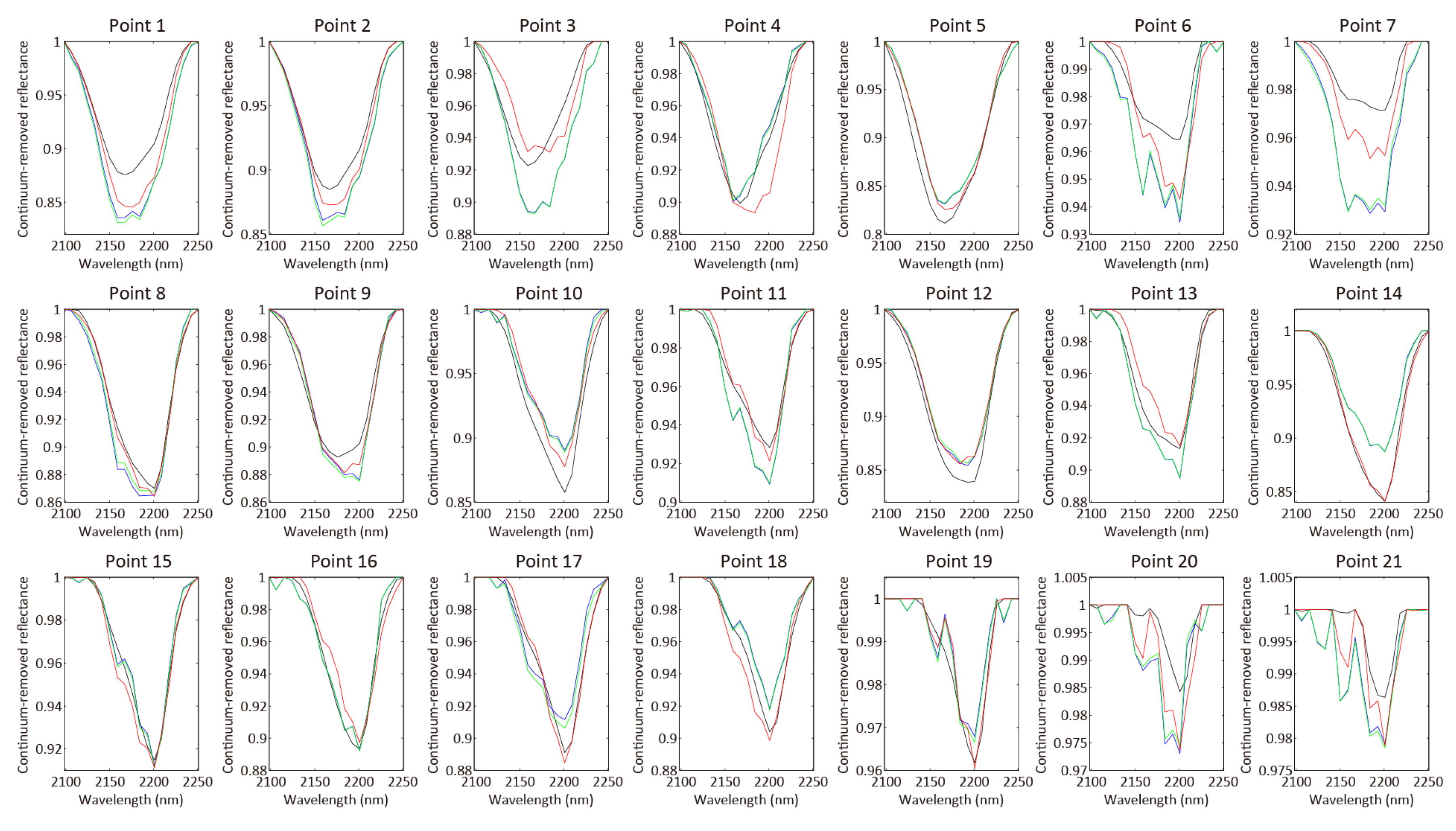
SAM is a measure for the shape preservation of a spectrum calculated at each pixel with a unit degree and 0 as the ideal value. An average value of a whole image is defined as
SAM ( X ^ , X ) = 1 P i = 1 P arccos ( x ^ i T x i x ^ i x i )
where x i denotes the i t h column vector of X and ‖·‖ is the l 2 norm.
(3)
RMSE is calculated at each pixel as the difference of spectra between the fused image and the reference image. We used an average value of RMSEs for all pixels, which is defined as
RMSE ( X ^ , X ) = 1 P j = 1 P 1 L i = 1 L ( X ^ i j X i j ) 2
For continuum-removed data, we consider a modified reference data ( X ) with each spectrum best matching its corresponding spectrum of the fused data to perform spectral feature fitting [42]. The modified continuum removed spectrum with scaling and shifting parameters at the i t h pixel is obtained by the least squares algorithm as x i = [ x i   1 L ] ( [ x i   1 L ] T [ x i   1 L ] ) 1 [ x i   1 L ] T x i , where 1 L L × 1 denotes a vector with all L entries one.
(4)
ERGAS provides a global statistical measure of the quality of fused data with the best value at 0, which is defined as
ERGAS ( X ^ , X ) = 100 P P h 1 L i = 1 L ( 1 P j = 1 P ( X ^ i j X i j ) 2 / 1 P j = 1 P X i j ) 2
The quality of the fused data products was validated with reflectance and continuum removal data using these measures of image quality and visual interpretations. Continuum removal is a technique that highlights useful information such as the shape and location of absorption peaks from background noise. As mineral materials often have subtle absorption features, continuum removal has been successfully applied to reflectance spectra [43,44].
We later show that the unmixing performance of the enhanced image is comparable to that of a “real” high-resolution hyperspectral image. Since the ground-truth data at a 10 m pixel level were not available, it was not possible to evaluate the precision of the unmixing. Instead, and probably more important for our purpose, the unmixing results from the enhanced 10 m hyperspectral image were visually compared with those from the 10 m hyperspectral reference image. Pixel spectra are also presented to show the correctness of the image fusion method.

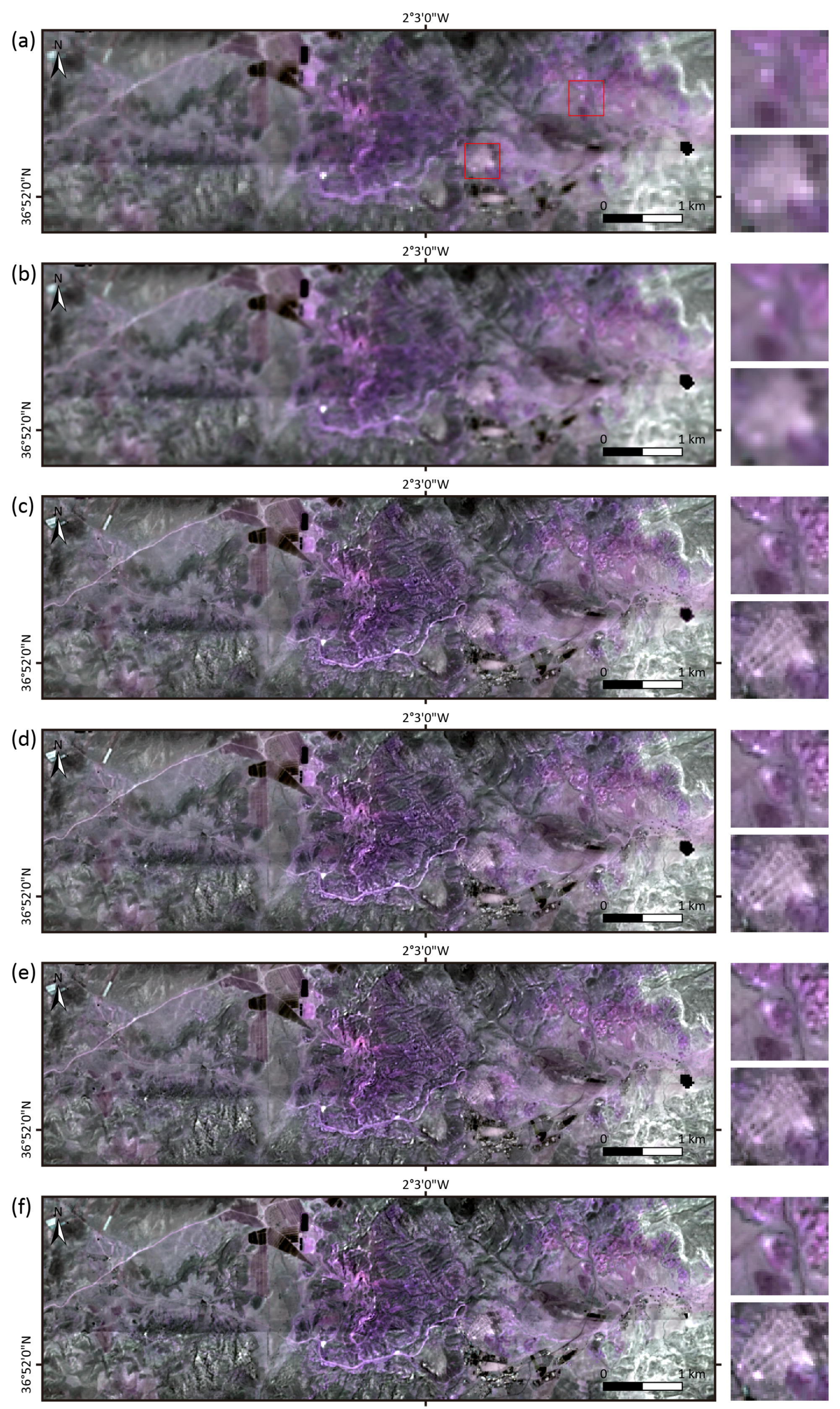
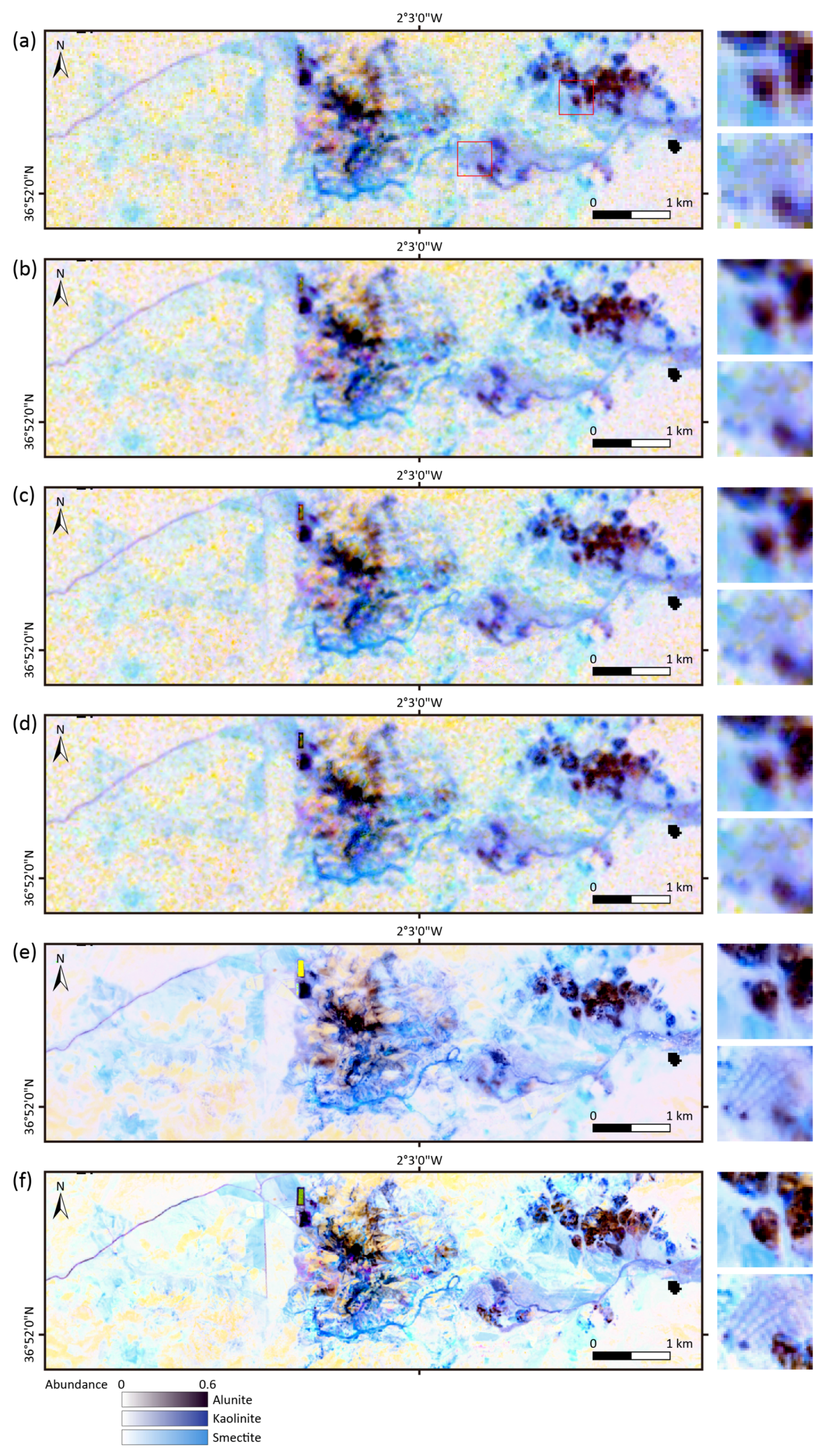
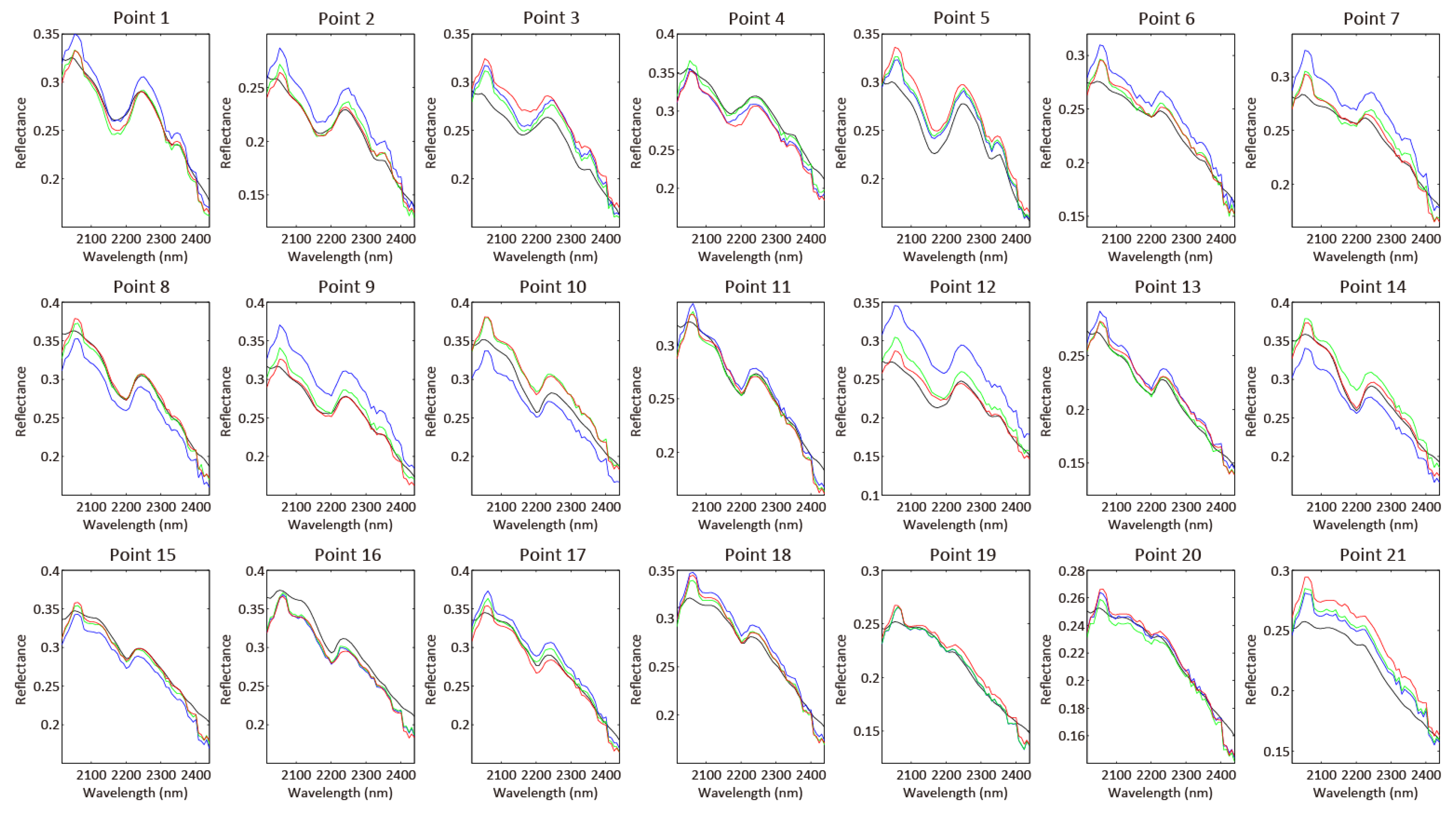
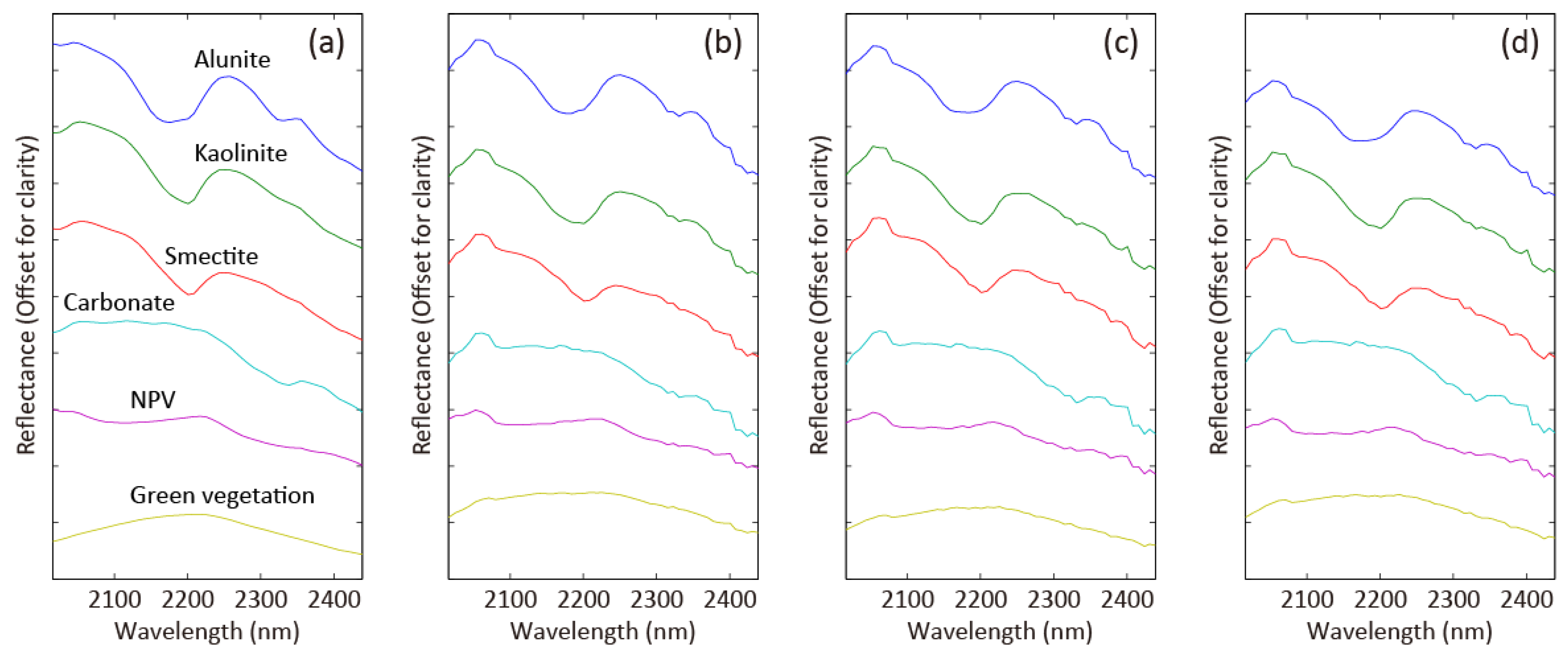
4. Results and Discussion

We fused Sentinel-2 bands 2, 3, 4 and 8 and EnMAP bands 1–127 and 189–242. In this way, a total of 181 high-resolution bands were simulated with 127 bands at 423–1335 nm, and 54 bands at 1998–2439 nm. Additionally, a 10 m hyperspectral reference image including the same EnMAP spectral bands was created. For mineral mapping, our analyses focused on the 52 SWIR bands between 2016–2439 nm. The quality indices are listed in Table 2 in three categories: (1) average over all the fused bands (both VNIR and SWIR); (2) average over fused bands in only the SWIR range; and (3) average over fused bands in only the SWIR range with continuum removal. The two pansharpening methods and the CNMF method achieved very similar scores in categories 1 and 2, but in category 3 with continuum removal the latter significantly outperformed the pansharpening methods.
Figure 3 shows a false-color composite comparison of the enhanced images and the reference image, where typical absorption feature bands at 2259, 2201 and 2014 nm are represented by red, green and blue channels, respectively. Two close-up images are also shown. A visual comparison suggests high-quality reconstruction using both the pansharpening methods and the CNMF method, and their results are clearly superior to those of single-frame nearest-neighbor interpolation and bicubic interpolation. The presence of target minerals (e.g., alunite, kaolinite, and smectite), indicated by shades of pink, is enhanced with the detailed spatial structure recovered through the high-resolution Sentinel-2 VNIR bands. There are, however, no major differences among the different methods according to the visual comparison. Absolute reflectance (or radiance) data have been commonly used for visual comparison in the literature of the resolution enhancement of hyperspectral images. However, absolute reflectance values, which appear as brightness in Figure 3, are heavily influenced by topography and solar elevation angles rather than actual mineralogy.
Figure 4 shows the visuals after continuum removal to demonstrate spectral absorption features at 2201, 2159 and 2115 nm. Black, blue and light blue are corresponding to alunite, kaolinite and smectite, respectively. The low abundances of kaolinite are indicated by pale purple. These correspondences were drawn from the analysis of spectral unmixing, which will be shown later. It is clear that CNMF generated results with finer detail. This is consistent with and has been verified by the quality indices in Table 2. The color composite images of the GSA and MTF-GLP data are surprisingly as blurred as that of the bicubic interpolation image. This is because of the high spectral correlation of the injected spectral vectors in the GSA and MTF-GLP data. More precisely, the injected detail vectors are parallel to each other in the centered data in the case of GSA, and the injected detail vector at each pixel is parallel to the corresponding resampled hyperspectral vector in the case of MTF-GLP. Spatial details are represented by the magnitudes of the injected vectors, which are normalized by continuum removal, resulting in their disappearance. The fact that the two pansharpening methods have no effect on resolution after continuum removal (Figure 4), which is hidden in reflectance (Figure 3), implies that continuum removal is effective to validate the fused hyperspectral data products. To our knowledge, this is the first study to demonstrate the efficacy of continuum removal for assessing the added value of hyperspectral image enhancement and to reveal the advantage of matrix-factorization-based image fusion as well as limitations of pansharpening.
To demonstrate spectral differences between the reference and enhanced images, we selected some exemplary spectra. We used the information of the 21 points reported in [37] to identify regions with different mineralogy. Since the exact coordinates were not available, the positions of these 21 points were estimated as accurately as possible as shown in the enlarged image in the bottom panel of Figure 1. Figure 5 shows the reflectance spectra generated from the different methods. The endmember spectra from the reference image are smoother because the reference image was generated by spectral resampling of the HyMap at-surface reflectance image without atmospheric simulation and correction (Figure 2), whereas those of the enhanced image products include errors resulting from a non-optimal atmospheric correction of the EnMAP image that is performed in the EnMAP end-to-end simulation. The spectra generated by bicubic interpolation show greater deviation at several locations. Otherwise, very good matching is achieved by both the pansharpening methods and the CNMF method with the useful information preserved. In Figure 6, the spectral signatures after continuum removal are shown. Better matching with CNMF than with the other methods is apparent. This is consistent with the obtained quality indices (Table 2) and the visual interpretation of Figure 4. At 10 m, CNMF appears to have been very effective for image fusion, most importantly, the reconstruction captures the absorption features crucial for mineral identification.
To further illustrate the potential of the enhanced image, the results of a spectral mixture analysis were used. Assuming that the spectral signal at each pixel is a weighted combination of endmembers, spectral unmixing methods have been proposed to resolve the fraction or abundance of each individual endmember [45]. While a normal realistic scene contains a large number of components, each having a distinctive spectral signature, an image pixel normally has only a few of these components mixed together. Although each pixel is a mixture of different numbers of components, simple spectral unmixing methods use a fixed number of endmembers, which can be problematic. Therefore, multiple-endmember unmixing [46] has been proposed and applied to the Rodalquilar scene in [37].
The first step of our spectral mixture analysis was endmember extraction. We adopted VCA to extract endmember candidates from the reference data and a final set of endmembers were manually selected by visual inspection, which resulted in six classes: alunite, kaolinite, smectite, carbonate, nonphotosynthetic vegetation (NPV) and green vegetation (Figure 7). Since the location of the endmembers in [37] was unknown, the endmember extraction was carefully processed by referring the spectral signatures of endmembers and their abundance maps in [37]. We extracted 25 endmember candidates from the reference data using VCA and manually selected five endmembers (alunite, kaolinite, smectite, NPV and green vegetation) considering their spectral similarity to those presented in [37], their locations and the corresponding abundance fractions shown in [37]. Only the spectral signature of carbonate was extracted fully by manually checking its locations with a high abundance fraction given in [37]. The six extracted spectra were used to unmix the reference image. Spatially corresponding spectra in the enhanced data were used as endmembers for spectral unmixing of the enhanced data.
Next, multiple endmember spectral mixture analysis (MESMA) [46] was applied to each reflectance image using respective endmember spectra to estimate the abundance fractions. We used photometric shade, with zero reflectance in all channels, as the shade endmember. Forty-one models with two to four endmembers were formed: six models with two endmembers (signature + shade), fifteen models with three endmembers (two signatures + shade) and twenty models with four endmembers (three signatures + shade). The constraint of the abundance fractions was set as −0.01 ≤ f ≤ 1.01. The maximum allowable RMSE was set to 0.01 in reflectance. Color composite images of abundance fractions for alunite (red), kaolinite (green) and smectite (blue) obtained using the reference, CNMF, GSA, bicubic interpolation, and nearest-neighbor interpolation images are shown in Figure 8. Although our results were generated using a 10 m image, they show good indicative resemblance to the results obtained from the 4 m hyperspectral image in [37]. Our primary goal is to show that the abundance fractions obtained using the fused data are comparable to those obtained from the reference image. The abundance fractions for the target minerals generated from the CNMF image and the reference image are highly comparable, although some spatial details are missing in the results obtained from the CNMF image. On the other hand, the results obtained using the GSA and bicubic interpolation images are more blurred, including different distributions of alunite due to spectral distortion. These results show for the first time that small spectral distortions included in resolution-enhanced hyperspectral data may have a major impact on spectral unmixing. This visual validation of the results of spectral unmixing has confirmed the efficacy of the CNMF method in addition to validating the numerical quality of enhanced images. The good resemblance of the results of spectral unmixing with that reported in [37] indicates the potential of CNMF-fused data in mineral mapping applications.

5. Conclusions

In this work, we investigated the potential of resolution-enhanced hyperspectral data for mineral mapping using a simulated pair of EnMAP and Sentinel-2 images. The EnMAP and Sentinel-2 products were generated from a HyMap scene covering a mining area using sensor end-to-end simulation tools, which take into account various instrumental and environmental configurations. The EnMAP and four Sentinel-2 VNIR bands were fused to produce a 10 m GSD hyperspectral image using the matrix factorization method that reconstructs the fused image via extraction of common underlying spectral signatures and their corresponding abundance fractions from the two images. The quality of resolution-enhanced hyperspectral data was validated by comparison with state-of-the-art pansharpening methods. Numerical quality measures and the visual interpretations using continuum-removed data demonstrated the high spectral and spatial fidelity with the presented method. The results of spectral unmixing showed highly comparable distributions with those generated from the reference image at a finer spatial resolution. These results suggested the effectiveness and potential of the presented hyperspectral and multispectral image fusion method. The contribution is a synergetic use of future EnMAP and Sentinel-2 data resulted in a spatial definition in geological exploration finer than those of the current and near future satellite missions such as EnMAP, the Japanese Hyperspectral Imager Suite (HISUI) [47], the Italian PRISMA (Hyperspectral Precursor of the Application Mission) [48], the US Hyperspectral Infrared Imager (HyspIRI) [49] and the French HYPXIM [50]. Naturally, the image fusion technique presented in this work can be extended to conventional applications such as detailed land cover classification and target detection; and with the enhanced data at 10 m GSD, there are potentially new applications that have not been anticipated for spaceborne hyperspectral remote sensing before.
In this study, we only used the 10 m Sentinel-2 VNIR bands to minimize the complexity of scaling, resulting in a challenging image fusion task without the overlap of SRFs in the SWIR range. In future work, the incorporation of the six additional 20 m SWIR bands will be further investigated to mitigate the ill-posedness of the inverse problem and improve the quality of the resolution-enhanced products. In addition, further experiments will be conducted based on better simulated sensor images from APEX and HySpex data with higher spectral and spatial resolutions. Clearly, further research will be required to validate the image fusion method with multi-sensor real data. The Multi-User System for Earth Sensing (MUSES) platform on the international space station is expected to provide a pair of hyperspectral and multispectral images acquired over the same area under the same environmental conditions, which satisfies the assumption of image fusion [51].

Acknowledgments

The authors would like to thank the reviewers for the many valuable comments and suggestions. This work was partially supported by the Kayamori Foundation of Information Science Advancement.

Author Contributions

Naoto Yokoya developed the methodology, conducted the experiments, and wrote the methodological and experimental parts of the manuscript. Jonathan Cheung-Wai Chan initiated the study, wrote the main flow of the manuscript, and revised the manuscript. Karl Segl prepared study data, provided useful suggestions, and revised the manuscript.

Conflicts of Interest

The authors declare no conflict of interest.

References

  1. Goetz, A.F.H.; Vane, G.; Solomon, J.E.; Rock, B.N. Imaging spectrometry for earth remote sensing. Science 1985, 228, 1147–1153. [Google Scholar] [CrossRef] [PubMed]
  2. Vane, G.; Goetz, A.F.H. Terrestrial imaging spectrometry: Current status, future trends. Remote Sens. Environ. 1993, 44, 117–126. [Google Scholar] [CrossRef]
  3. Hunt, G.R. Spectral signatures of particulate minerals in the visible and near infrared. Geophysics 1977, 42, 501–513. [Google Scholar] [CrossRef] [Green Version]
  4. Clark, R.N.; Swayze, G.A.; Livo, K.E.; Kokaly, R.F.; Sutley, S.J.; Dalton, J.B.; Mcdougal, R.R.; Gent, C.A. Imaging spectroscopy: Earth and planetary remote sensing with the USGS Tetracorder and expert systems. J. Geophys. Res. Planets 2003, 108. [Google Scholar] [CrossRef]
  5. Kruse, F.A.; Boardman, J.W.; Huntington, J.F. Comparison of airborne hyperspectral data and EO-1 Hyperion for mineral mapping. IEEE Trans. Geosci. Remote Sens. 2003, 41, 1388–1400. [Google Scholar] [CrossRef]
  6. Van der Meer, F.; Van der Werff, H.; Frank, J.A.; Van Ruitenbeek, F.; Hecker, C.A.; Bakker, W.H.; Noomen, M.F.; van der Meijde, M.; Carranza, E.J.M.; Boudewijn de Smeth, J.; et al. Multi- and hyperspectral geologic remote sensing: A review. Int. J. Appl. Earth Obs. Geoinf. 2012, 14, 112–128. [Google Scholar] [CrossRef]
  7. Guanter, L.; Kaufmann, H.; Segl, K.; Förster, S.; Rogaß, C.; Chabrillat, S.; Küster, T.; Hollstein, A.; Rossner, G.; Chlebek, C.; et al. The EnMAP spaceborne imaging spectroscopy mission for earth observation. Remote Sens. 2015, 7, 8830–8857. [Google Scholar] [CrossRef]
  8. Pearlman, J.S.; Barry, P.S.; Segal, C.C.; Shepanski, J.; Beiso, D.; Carman, L. Hyperion, a space-based imaging spectrometer. IEEE Trans. Geosci. Remote Sens. 2003, 41, 1160–1173. [Google Scholar] [CrossRef]
  9. Akgun, T.; Altunubasak, Y.; Mersereau, R.M. Super-resolution enhancement of hyperspectral CHRIS/Proba images with a thin-plate spline non-rigid transform model. IEEE Trans. Geosci. Remote Sens. 2005, 48, 1860–1875. [Google Scholar]
  10. Chan, J.C.-W.; Ma, J.; Kempeneers, P.; Canters, F. Superresolution reconstruction of hyperspectral images. IEEE Trans. Geosci. Remote Sens. 2005, 14, 2569–2579. [Google Scholar]
  11. Gu, Y.; Zhang, Y.; Zhang, J. Integration of spatial-spectral information for resolution enhancement in hyperspectral images. IEEE Trans. Geosci. Remote Sens. 2008, 46, 1347–1358. [Google Scholar]
  12. Zhao, Y.; Zhang, L.; Kong, S.G. Band-subset-based clustering and fusion for hyperspectral imagery classification. IEEE Trans. Geosci. Remote Sens. 2011, 49, 747–756. [Google Scholar] [CrossRef]
  13. Vivone, G.; Alparone, L.; Chanussot, J.; Dalla Mura, M.; Garzelli, M.; Licciardi, G. A critical comparison among pansharpening algorithms. IEEE Trans. Geosci. Remote Sens. 2015, 53, 2565–2586. [Google Scholar] [CrossRef]
  14. Loncan, L.; Almeida, L.B.; Bioucas-Dias, J.; Briottet, X.; Chanussot, J.; Dobigeon, N.; Fabre, S.; Liao, W.; Licciardi, G.A.; Simoes, M.; et al. Hyperspectral pansharpening: A review. IEEE Geosci. Remote Sens. Mag. 2015, 3, 27–46. [Google Scholar] [CrossRef]
  15. Hardie, R.C.; Eismann, M.T.; Wilson, G.L. MAP estimation for hyperspectral image resolution enhancement using an auxiliary sensor. IEEE Trans. Image Process. 2004, 13, 1174–1184. [Google Scholar] [CrossRef] [PubMed]
  16. Eismann, M.T.; Hardie, R.C. Application of the stochastic mixing model to hyperspectral resolution enhancement. IEEE Trans. Geosci. Remote Sens. 2004, 42, 1924–1933. [Google Scholar] [CrossRef]
  17. Zhang, Y.; Backer, S.D.; Scheunders, P. Noise-resistant wavelet based Bayesian fusion of multispectral and hyperspectral images. IEEE Trans. Geosci. Remote Sens. 2009, 47, 3834–3843. [Google Scholar] [CrossRef]
  18. Yokoya, N.; Yairi, T.; Iwasaki, A. Coupled nonnegative matrix factorization unmixing for hyperspectral and multispectral data fusion. IEEE Trans. Geosci. Remote Sens. 2012, 50, 528–537. [Google Scholar] [CrossRef]
  19. Kawakami, R.; Wright, J.; Tai, Y.; Matsushita, Y.; Ben-Ezra, M.; Ikeuchi, K. High-resolution hyperspectral imaging via matrix factorization. In Proceedings of the IEEE International Conference Computer Vision and Pattern Recognition (CVPR), Colorado Springs, CO, USA, 21–23 June 2011; pp. 2329–2336.
  20. Veganzones, M.; Simes, M.; Licciardi Yokoya, N.; Bioucas-Dias, J.M.; Chanussot, J. Hyperspectral super-resolution of locally low rank images from complementary multisource data. IEEE Trans. Image Process. 2016, 25, 274–288. [Google Scholar] [CrossRef] [PubMed]
  21. Simoes, M.; Bioucas-Dias, J.M.; Almeida, L.; Chanussot, J. A convex formulation for hyperspectral image superresolution via subspace-based regularization. IEEE Trans. Geosci. Remote Sens. 2015, 53, 3373–3388. [Google Scholar] [CrossRef]
  22. Wei, Q.; Bioucas-Dias, J.M.; Dobigeon, N.; Tourneret, J.-Y. Hyperspectral and multispectral image fusion based on a sparse representation. IEEE Trans. Geosci. Remote Sens. 2015, 53, 3658–3668. [Google Scholar] [CrossRef]
  23. Chen, Z.; Pu, H.; Wang, B.; Jiang, G.-M. Fusion of hyperspectral and multispectral images: A novel framework based on generalization of pan-sharpening methods. IEEE Geosci. Remote Sens. Lett. 2014, 11, 1418–1422. [Google Scholar] [CrossRef]
  24. Grohnfeldt, C.; Zhu, X.; Bamler, R. The J-SparseFI-HM hyperspectral resolution enhancement method—Now fully automated. In Proceedings of the IEEE Workshop Hyperspectral Image Signal Process: Evolution in Remote Sens. (WHISPERS), Lausanne, Switzerland, 24–27 June 2014; pp. 1–4.
  25. Van der Meer, F.D.; Van der Werff, H.M.A.; Van Ruitenbeek, F.J.A. Potential of ESA’s Sentinel-2 for geological applications. Remote Sens. Environ. 2014, 148, 124–133. [Google Scholar] [CrossRef]
  26. Guanter, L.; Segl, K.; Kaufmann, H. Simulation of optical remote sensing scenes with application to the EnMAP hyperspectral mission. IEEE Trans. Geosci. Remote Sens. 2009, 47, 2340–2351. [Google Scholar] [CrossRef]
  27. Segl, K.; Guanter, L.; Kaufmann, H. Simulation of spatial sensor characteristics in the context of the EnMAP hyperspectral mission. IEEE Trans. Geosci. Remote Sens. 2010, 48, 3046–3054. [Google Scholar] [CrossRef]
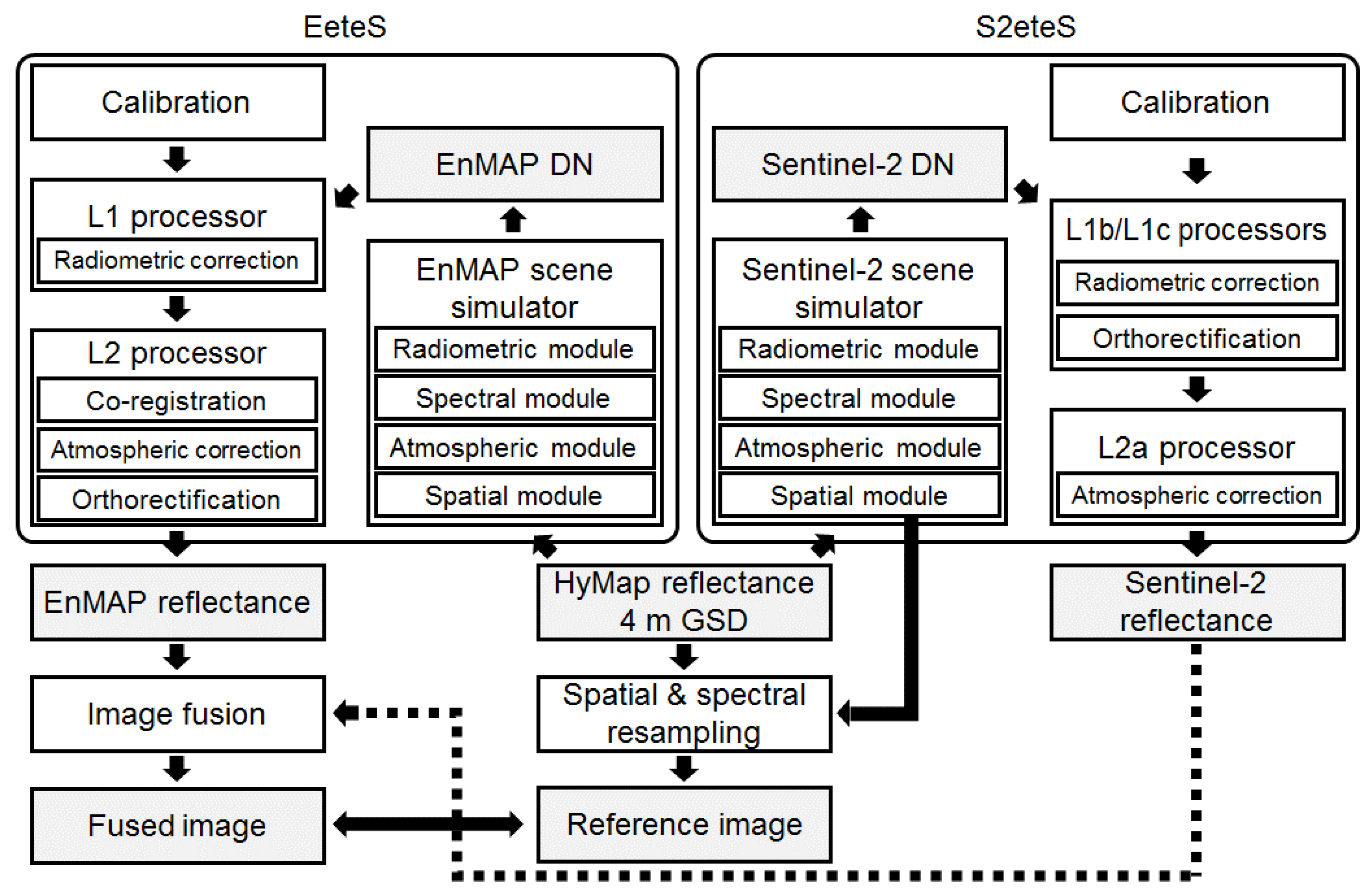
  28. Segl, K.; Guanter, L.; Rogass, C.; Kuester, T.; Roessner, S.; Kaufmann, H.; Sang, B.; Mogulsky, V.; Hofer, S. EeteS—The EnMAP end-to-end simulation tool. IEEE J. Sel. Topics Appl. Earth Obs. Remote Sens. 2012, 5, 522–530. [Google Scholar] [CrossRef]
  29. Segl, K.; Guanter, L.; Gascon, F.; Kuester, T.; Rogass, C.; Mielke, C. S2eteS—An end-to-end modelling tool for the simulation of Sentinel-2 image products. IEEE Trans. Geosci. Remote Sens. 2015, 53, 5560–5571. [Google Scholar] [CrossRef]
  30. Gomez, G.; Jazaeri, A.; Kafatos, M. Wavelet-based hyperspectral and multi-spectral image fusion. Proc. SPIE 2001. [Google Scholar] [CrossRef]
  31. Zhang, Y.; He, M. Multi-spectral and hyperspectral image fusion using 3-D wavelet transform. J. Electron. 2007, 24, 218–224. [Google Scholar] [CrossRef]
  32. Yokoya, N.; Mayumi, N.; Iwasaki, A. Cross-calibration for data fusion of EO-1/Hyperion and Terra/ASTER. IEEE J. Sel. Topics Appl. Earth Obs. Remote Sens. 2013, 6, 419–426. [Google Scholar] [CrossRef]
  33. Bioucas-Dias, J.M.; Plaza, A.; Dobigeon, N.; Parente, M.; Du, Q.; Gader, P.; Chanussot, J. Hyperspectral unmixing overview: Geometrical, statistical, and sparse regression-based approaches. IEEE J. Sel. Top. Appl. Earth Obs. Remote Sens. 2012, 5, 354–379. [Google Scholar] [CrossRef]
  34. Lee, D.D.; Seung, H.S. Learning the parts of objects by nonnegative matrix factorization. Nature 1999, 401, 788–791. [Google Scholar] [PubMed]
  35. Lee, D.D.; Seung, H.S. Algorithms for non-negative matrix factorization. In Proceedings of the Conference Advertising Neural Information Processing System, Vancouver, BC, Canada, 3–8 December 2001; Volume 13, pp. 556–562.
  36. Nascimento, J.M.P.; Bioucas-Dias, J.M. Vertex component analysis: A fast algorithm to unmix hyperspectral data. IEEE Trans. Geosci. Remote Sens. 2005, 43, 898–910. [Google Scholar] [CrossRef]
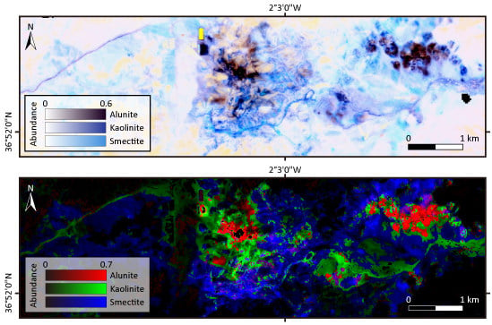
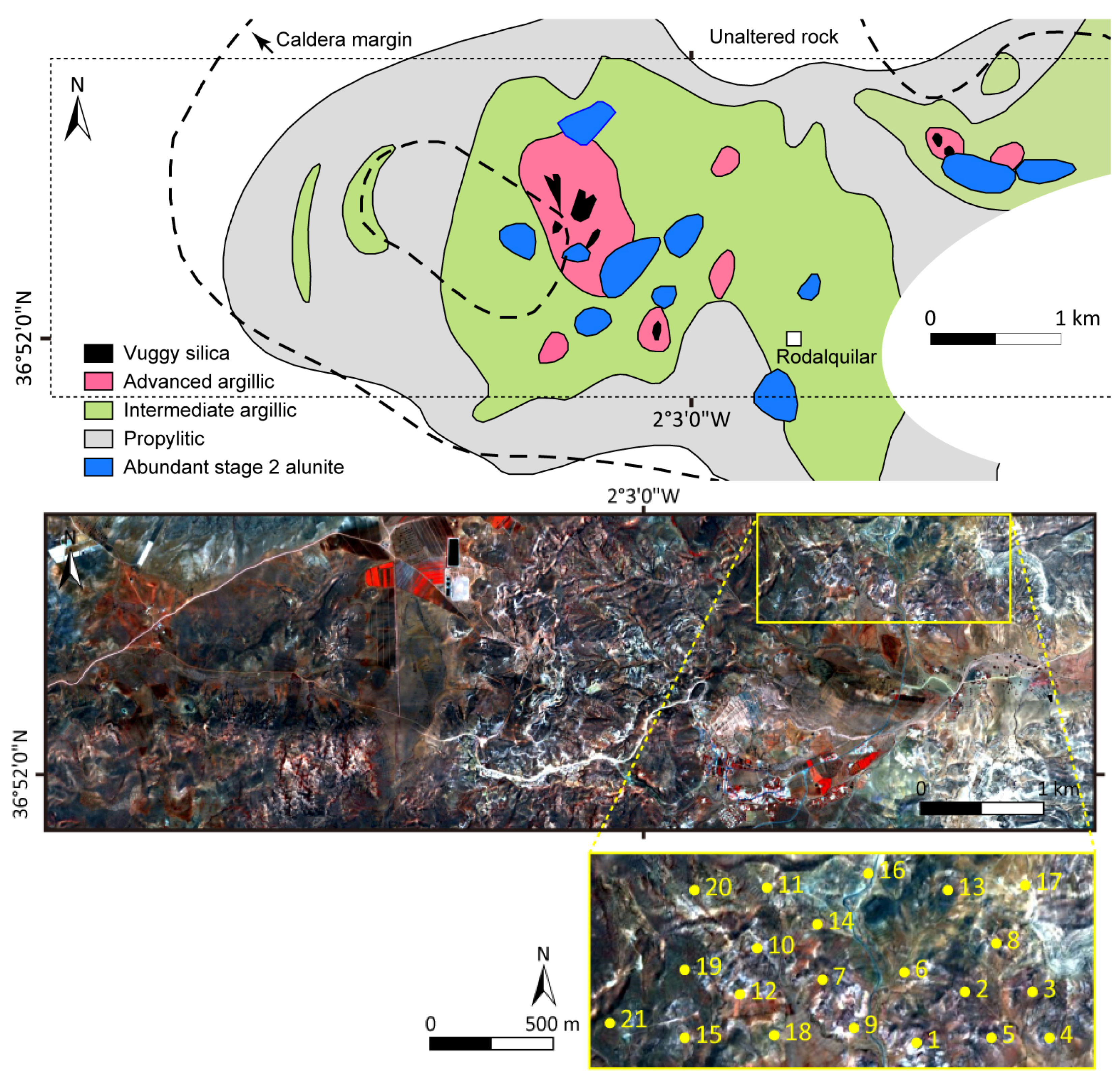
  37. Bedini, E.; Van der Meer, F.; Van Ruitenbeek, F. Use of HyMap imaging spectrometer data to map mineralogy in the Rodalquilar caldera, southeast Spain. Int. J. Remote Sens. 2009, 30, 327–348. [Google Scholar] [CrossRef]
  38. Arribas, A.; Cunningham, C.G.; Rytuba, J.J.; Rye, R.O.; Kelly, W.C.; Podwysocki, M.H.; Mckee, E.H.; Tosdal, R.M. Geology, geochronology, fluid inclusions, and isotope geochemistry of the Rodalquilar gold alunite deposit, Spain. Econ. Geol. Bull. Soc. Econ. Geol. 1995, 90, 795–822. [Google Scholar] [CrossRef]
  39. Aiazzi, B.; Baronti, S.; Selva, M. Improving component substitution pansharpening through multivariate regression of MS+Pan data. IEEE Trans. Geosci. Remote Sens. 2007, 45, 3230–3239. [Google Scholar] [CrossRef]
  40. Aiazzi, B.; Alparone, L.; Baronti, S.; Garzelli, A.; Selva, M. MTF tailored multiscale fusion of high-resolution MS and Pan imagery. Photogramm. Eng. Remote Sens. 2006, 72, 591–596. [Google Scholar] [CrossRef]
  41. Wald, L. Quality of high resolution synthesized images: Is there a simple criterion? In Proceedings of the Third Conference “Fusion of Earth Data”, Sophia Antipolis, France, 26–28 January 2000; pp. 99–105.
  42. Clark, R.N.; Gallagher, A.J.; Swayze, G.A. Material absorption band depth mapping of imaging spectrometer data using a complete band shape least-squares fit with library reference spectra. In Proceedings of the Second Airborne Visible/Infrared Imaging Spectrometer (AVIRIS) Workshop, Pasadena, CA, USA, 4–5 June 1990; pp. 176–186.
  43. Singer, R.B. Near-infrared spectral reflectance of mineral mixtures: Systematic combinations of pyroxenes, olivine, and iron oxides. J. Geophys. Res. 1981, 86, 7967–7982. [Google Scholar] [CrossRef]
  44. Clark, R.N.; Roush, T.L. Reflectance spectroscopy-quantitative analysis techniques for remote-sensing applications. J. Geophys. Res. 1984, 89, 6329–6340. [Google Scholar] [CrossRef]
  45. Adams, J.B.; Smith, M.O.; Johnson, P.E. Spectral mixture modeling: A new analysis of rock and soil types at the Viking Lander 1 site. J. Geophys. Res. 1986, 91, 8098–8112. [Google Scholar] [CrossRef]
  46. Roberts, D.A.; Gadner, M.; Church, R.; Ustin, S.; Scheer, G.; Green, O.R. Mapping chaparral in the Santa Monica mountains using multiple endmember spectral mixture models. Remote Sens. Environ. 1998, 65, 267–279. [Google Scholar] [CrossRef]
  47. Iwasaki, A.; Ohgi, N.; Tanii, J.; Kawashima, T.; Inada, H. Hyperspectral imager suite (HISUI)-Japanese hyper-multi spectral radiometer. In Proceedings of the International Geoscience Remote Sensing Symptom (IGARSS), Vancouver, BC, Canada, 24–29 July 2011; pp. 1025–1028.
  48. Stefano, P.; Angelo, P.; Simone, P.; Filomena, R.; Federico, S.; Tiziana, S.; Umberto, A.; Vincenzo, C.; Acito, N.; Marco, D.; et al. The PRISMA hyperspectral mission: Science activities and opportunities for agriculture and land monitoring. In Proceedings of the International Geoscience Remote Sensing Symptom (IGARSS), Melbourne, Australia, 21–26 July 2013; pp. 4558–4561.
  49. Green, R.; Asner, G.; Ungar, S.; Knox, R. NASA mission to measure global plant physiology and functional types. In Proceedings of the Aerospace Conference, Big Sky, MT, USA, 1–8 March 2008; pp. 1–7.
  50. Michel, S.; Gamet, P.; Lefevre-Fonollosa, M.J. HYPXIM—A hyperspectral satellite defined for science, security and defence users. In Proceedings of the IEEE Workshop Hyperspectral Image Signal Processing: Evolution in Remote Sensing (WHISPERS), Lisbon, Portugal, 6–9 June 2011; pp. 1–4.
  51. Eckardt, A.; Horack, J.; Lehmann, F.; Krutz, D.; Drescher, J.; Whorton, M.; Soutullo, M. DESIS (DLR Earth sensing imaging spectrometer for the ISS-MUSES platform. In Proceedings of the International Geoscience Remote Sensing Symptom (IGARSS), Milan, Italy, 26–31 July 2015; pp. 1457–1459.
Figure 1. Top: Schematic surface alteration map of the study area (modified from [38]). The dotted rectangle indicates the approximate outline of the study area; Bottom: The scene is displayed in false color composite (R: 750 nm, G: 550 nm, B: 450 nm) made from the original HyMap image. Bright red represents cultivated cropland, and shades of red show distribution of various vegetated land covers. Numbered points in the enlarged image are 21 locations for validation of spectral signatures [37].
Remotesensing 08 00172 g001
Figure 2. Flowchart of data preparation.
Remotesensing 08 00172 g002
Figure 3. Color composite images (R: 2259 nm, G: 2201 nm, B: 2044 nm) obtained by (a) nearest-neighbor interpolation; and (b) bicubic interpolation of EnMAP data, and fusion of EnMAP and Sentinel-2 data using (c) GSA; (d) MTF-GLP; (e) CNMF; and (f) reference data. Shades of pink indicate the presence of minerals, such as alunite, kaolinite and smectite, Monotone areas indicate no absorption feature in the spectral range between 2259 nm and 2044 nm and brightness is influenced by topography and the sun elevation angle in addition to variations of land cover.
Remotesensing 08 00172 g003
Figure 4. Color composite images (R: 2201 nm, G: 2159 nm, B: 2115 nm) of continuum removed images obtained by (a) nearest-neighbor interpolation; and (b) bicubic interpolation of EnMAP data; and fusion of EnMAP and Sentinel-2 data using (c) GSA; (d) MTF-GLP; (e) CNMF; and (f) reference data. Black, blue and light blue are corresponding to alunite, kaolinite and smectite, respectively.
Remotesensing 08 00172 g004
Figure 5. Comparison of spectral signatures between (black) reference; (blue) bicubic interpolation; (green) GSA; and (red) CNMF images at 21 points [37].
Remotesensing 08 00172 g005
Figure 6. Comparison of continuum-removed spectral signatures between (black) reference; (blue) bicubic interpolation; (green) GSA; and (red) CNMF images at 21 points [37].
Remotesensing 08 00172 g006
Figure 7. Endmember spectra derived from (a) reference; (b) CNMF; (c) GSA; and (d) bicubic interpolation data.
Remotesensing 08 00172 g007
Figure 8. Color composite images of abundance fractions obtained from (a) nearest-neighbor interpolation; (b) bicubic interpolation; (c) GSA; (d) CNMF; and (e) reference images by MESMA for alunite (red); kaolinite (green); and smectite (blue). Abundance fractions are linearly stretched between 0 to 0.7 for better visualization.
Remotesensing 08 00172 g008aRemotesensing 08 00172 g008b
Table 1. Spectral bands for the Sentinel-2 sensor.
Band NumberCentral Wavelength (nm)Bandwidth (nm)GSD (m)
14432060
24906510
35603510
46653010
57051520
67401520
77832020
884211510
8b8652020
99452060
1013803060
1116109020
12219018020
Table 2. Quality indices.
DataMethodCCSAMRMSEERGAS
VNIR and SWIRCubic0.917492.83650.019093.3857
GSA0.986292.7130.013722.0112
MTF-GLP0.985712.6920.013552.0151
CNMF0.9882.69940.013491.9793
SWIRCubic0.905491.63680.016942.9814
GSA0.973741.6290.011491.9339
MTF-GLP0.973461.63810.011321.8958
CNMF0.973291.61930.011651.9336
Continuum removed SWIRCubic0.765780.655530.010150.45248
GSA0.77450.648320.010110.4504
MTF-GLP0.76590.661410.010190.46186
CNMF0.834940.607610.009150.40899

