Spatial-Temporal Dynamics of China’s Terrestrial Biodiversity: A Dynamic Habitat Index Diagnostic

Abstract

Biodiversity in China is analyzed based on the components of the Dynamic Habitat Index (DHI). First, observed field survey based spatial patterns of species richness including threatened species are presented to test their linear relationship with remote sensing based DHI (2001–2010 MODIS). Areas with a high cumulative DHI component are associated with relatively high species richness, and threatened species richness increases in regions with frequently varying levels of the cumulative DHI component. The analysis of geographical and statistical distributions yields the following results on interdependence, polarization and change detection: (1) The decadal mean Cumulative Annual Productivity (DHI-$\overline{cum}$ < 4) in Northwest China and (DHI-$\overline{cum}$ > 4) in Southeast China are in a stable (positive) relation to the Minimum Annual Apparent Cover (DHI-$\overline{min}$) and is positively (negatively) related to the Seasonal Variation of Greenness (DHI-$\overline{sea}$); (2) The decadal tendencies show bimodal frequency distributions aligned near DHI-$\overline{min}$~0.05 and DHI-$\overline{sea}$~0.5 which separated by zero slopes; that is, regions with both small DHI-min and DHI-sea are becoming smaller and vice versa; (3) The decadal tendencies identify regions of land-cover change (as revealed in previous research). That is, the relation of strong and significant tendencies of the three DHI components with climatic or anthropogenic induced changes provides useful information for conservation planning. These results suggest that the spatial-temporal dynamics of China’s terrestrial species and threatened species richness needs to be monitored by first and second moments of remote sensing based information of the DHI.

1. Introduction

Global extinction rates have increased due to anthropogenic activities [1,2,3,4,5], which have led to an erosion of ecosystem services [6]. Efforts to reduce this rapid biotic impoverishment have been carried out by many countries in terms of enacting, or planning to enact, legislation for the identification, protection, and recovery of endangered species [5,7,8,9]. The Chinese government has initiated several environmental programs to increase its commitment to environmental protection, including the National Forest Conservation Program (NFCP, 2000; see [10]) and the Grain-to-Green Program (GTGP, 1999; see [11]). However, these programs are carried out statewide so that methods of implementation as well as their effectiveness vary among different areas [12].

Regional evaluation and measurements for habitat conservation, species and endangered species richness still remain poorly integrated into these programs, particularly outside nature reserves [13,14]. Therefore, reliable information about the geographic distribution of species richness and endangered species is necessary. At present, there are three methodologies for measuring species richness and endangered species from sources: they are obtained from field surveys (also called the meta-analysis approach, see [15]); estimated from existing land cover maps by combining information about the known habitat requirements of species [16,17,18], e.g., the USGS National Gap Analysis Program [19]; and derived from remote sensing based indices that consider the relationship between spectral radiance and species richness, e.g., Dynamic Habitat Index DHI [20,21,22]. For applications to extensive and complex land surface areas these methodologies show the following characteristics:

(1) The meta-analysis approach uses the emergent outcome of numerous tests by compiling the results of previously published analyses [15]. It assumes that different areas of ecology share the same sampling system and design properties, although their regional ecologies are virtually unique from study to study [23].

(2) Land cover map analyses extract species occurrences by considering the composition, abundance and distribution requirements of individual species or assemblages with maps of land cover [24]. The pace of land habitat loss and conversion (provided by remotely sensed imagery) allows estimates of the related biodiversity loss [16,17,18]. Compatibility of current state analyses and future projections, and/or of different spatial resolution of land cover systems could be an issue, in particular, when assumptions about missing information have to be made. The project “Geo-Wiki” provides a platform where citizens help in validating global land cover maps [25,26,27], which may lead to improvements in this methodology by using validated land cover maps.

(3) Remote sensing based Dynamic Habitat Index-based analyses propose a relationship between spectral radiance and species richness. The usefulness of DHI has been tested in previous validation research using actual biodiversity data [20] (originally proposed by Mackey et al. [21] and Berry et al. [28]), which show that there is a direct linear relationship between vegetation productivity and the richness of specific species. DHI analysis has been applied to Canada [20,22,29] and North American [30]. Spatial and seasonally induced variation in DHI are closely related to the patterns of avian species richness with highest correlations up to 88% [31]. Furthermore, in combination with long-term climate change, DHI can be used to assess the long-term variability of vegetation biodiversity [32]. However, the index is for the first time being applied in China. Assuming that DHI constitutes a surrogate species richness without testing relationships with actual species richness may be incorrect and could be misleading when expanding the analysis to endangered species richness.

The relationship between DHI components and species richness has been demonstrated in a number of studies to estimate the richness of breeding bird species in the United States and Canada [22,30,31,33]. In this study we focus on estimating the species distribution, its change and variability using DHI information. In addition, we expand the original DHI components (related with avian species) to: (1) a relationship that combines mammals, birds, and amphibians; (2) a grid-scale (10 × 10 km²) based analysis for further enhancing the spatial resolution; and (3) a dynamic change and variability analysis associated with the static species richness information obtained from annual climate means.

Therefore, we first revisit the DHI components (in Section 2) and then test the relationship between the spatial patterns of indices derived from remote sensing information as possible surrogates of biodiversity and of the actual overall species richness and threatened species richness in China (in Section 3). This includes the distributions of species richness and threatened species richness and the distributions of change tendencies, from 2001 to 2010. A discussion and summary conclude the analysis (Section 4).

2. Data and Methodology

2.1. Data

The Fraction of Absorbed Photosynthetically Active Radiation (fPAR) time series from MODIS (MOD15A2, 2001–2010) is used in this study. The fPAR data is provided every 8 days at 1 × 1 km² spatial resolution as a gridded level-4 product in the sinusoidal projection. Data processing involves the calibration of sensor changeover and corrections to remove the effects of sensor degradation, satellite orbit drift, solar zenith angles, and other factors [34]. Species and threatened species census (2013, types/10 × 10 km²) of mammals and amphibians from the International Union for Conservation of Nature, and of birds from BirdLife International and NatureServe [35,36] are added to account for the relationship between field survey datasets and the remote sensing derived surrogate of species richness and threatened species richness (see Figure 1, data available from the website [37]).

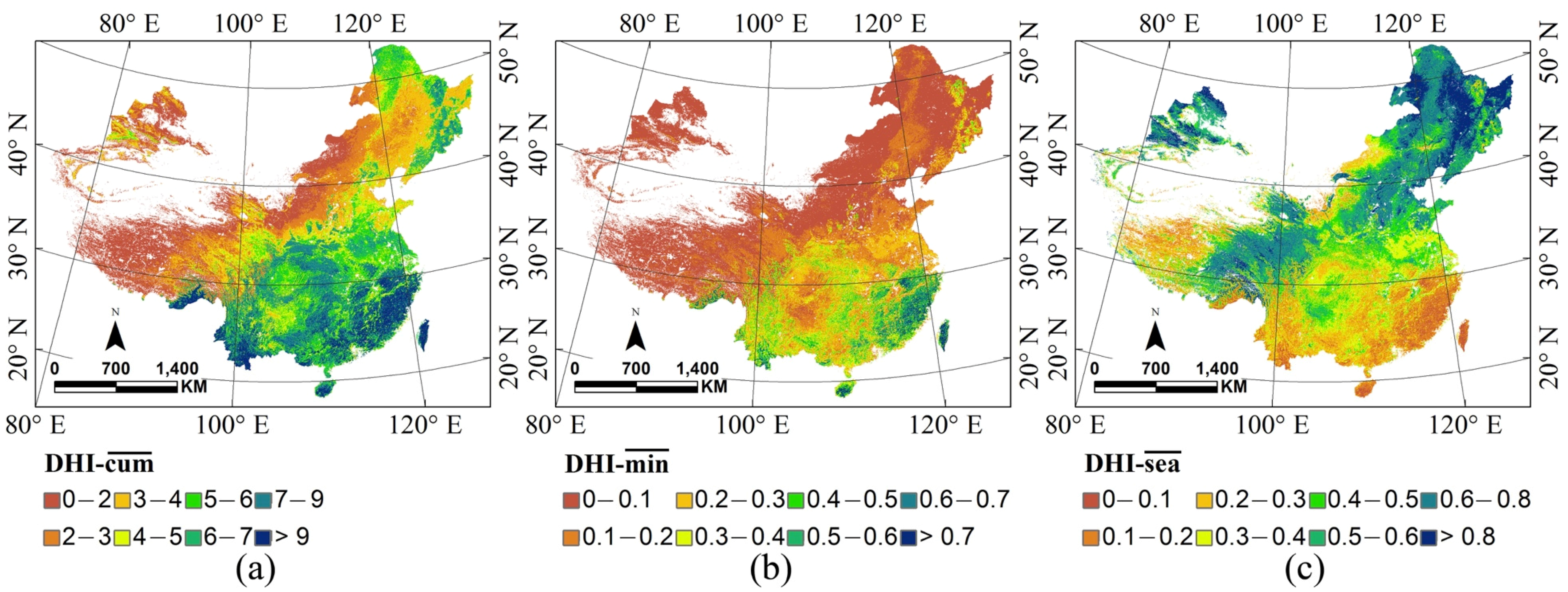
2.2. Dynamic Habitat Index

The dynamic habitat index (DHI-(cum,min,sea)) is a composite vector deduced from fPAR time series, representing the underlying vegetation dynamics [20], where fPAR is expressed as a non-dimensional fraction of incoming radiation received by the land surface. Monthly maximum fPAR-values on 1 × 1 km² resolution are the basic input data set to compute the three relevant annual indices for the subsequent habitat analysis (Section 3).

(1) Cumulative Annual Productivity (DHI-cum), which is estimated by summing all monthly fPAR values for each year, indirectly explains species distribution and abundance, because it characterizes the supply of resources like food supply [22,38,39]. This is an annual total of all monthly productivity contributions:

$$DHI-cum={{\displaystyle \sum }}_{month}MA{X}_{layer,fPAR}$$

(1)

(2) Minimum Annual Apparent Cover (DHI-min) represents the lowest (minimum value) level of vegetative cover in a year, it indicates the capacity of the landscape to sustain an adequate level of food and habitat resources during this period [22,40]. This annual value represents the monthly minimum productivity of the year:

$$DHI-min=MIN\left\{{\left(MA{X}_{layer,fPAR}\right)}_{month},\dots \right\}$$

(2)

(3) Seasonal Variation of Greenness (DHI-sea) refers to a surrogate of habitat quality associated with its relationship to natural resources (e.g., food, water and nutrients), it is expected to exert selective pressure on life history traits [41,42]. This annual index represents a coefficient of variability to characterize the month-to-month standard deviation in relation to its annual mean:

$$DHI-sea=\frac{STD\left\{{\left(MA{X}_{layer,fPAR}\right)}_{month},\dots \right\}}{MEAN\left\{{\left(MA{X}_{layer,fPAR}\right)}_{month},\dots \right\}}$$

(3)

where layer is an index representing individual fPAR dataset of 8 days temporal resolution. For each month, MAX_layer,fPAR represents a monthly maximum value calculated by the Maximum Value Composite methodology [43]. MIN, MEAN and STD are the minimum, mean and standard deviation of monthly maximum values in a particular year. A ten-year mean climatology (DHI-($\overline{cum},\overline{min},\overline{sea}$)) will be calculated to represent a long-term average state (or climate mean).

2.3. Regression Tendency Analysis

To estimate the long-term vegetation dynamics (2001–2010), a simple linear regression analysis by least squares [44,45] is applied to yearly DHI-(cum,min,sea).

$$Slop{e}_i=\frac{N\times {\sum }_{n=1}^{N}n\times DH{I}_i-\left({\sum }_{n=1}^{N}n\right)\left({\sum }_{n=1}^{N}DH{I}_i\right)}{N\times {\sum }_{n=1}^N{n}^2-{\left({\sum }_{n=1}^{N}n\right)}^2}$$

(4)

where Slope_i is the slope of the regression line of DHI_i ~ DHI-(cum,min,sea), $i\in \left\{1,2,3\right\}$. $n\in \left\{1,2,\dots ,10\right\}$ represents the number of year. The trend of DHI_i increases (decreases) when Slope_i is positive (negative).

2.4. Decadal Mean and Inter-Annual Variability

Transforming the input time series data into the DHI vector is a critical step for testing the usefulness whether the DHI constitutes a useful surrogate about species richness. A direct linear relationship between the DHI and particular species richness has been documented [31,33]. However, the inter-annual variability of long-term DHI components, namely the standard deviation of DHI-cum has, to our knowledge, not been implemented into this dynamic analysis nor have any suggestions been made on how to introduce it. Therefore, in this study, the following three-step procedure was developed to derive not only a remote sensing based surrogate of species but also to implement a novel procedure using the inter-annual coefficient of variability to obtain a surrogate of threatened species richness for global/regional application (application in China, see Section 3):

Step-1: Data-preprocessing: ArcGIS© 10.1 software was used to relate/combine and resample MODIS based DHI components (1 × 1 km²) in order to obtain a comparable spatial resolution with 10 × 10 km² of actual field survey based species and threatened species richness.

Step-2: Remote sensing surrogate for species richness: The decadal mean of DHI-cum is used to test the assumption that the DHI-cum constitutes a surrogate of species richness at the regional/continental scale for further classifying species richness in large areas and their changes through time based on a simple linear regression model: DHI-$\overline{cum}$ = a₁ × actual species richness + a₀. Linear regression analysis is employed to relate remote sensing-based information (DHI-$\overline{cum}$) to field survey based species richness.

Step-3: Remote sensing surrogate for endangered species richness: The standard deviation SD of DHI-cum is compared with the field survey data of richness of threatened species to analyze its potential as a remote sensing based surrogate of threatened species richness by employing a simple linear regression: SD(DHI-cum) = b₁ × actual endangered species richness + b₀. The confirmation of the linear relationship is achieved through the R² and p-value of the regression, which reveals that SD(DHI-cum) is a possible remote sensing surrogate for endangered species richness.

3. Application of the Dynamic Habitat Analysis: Results for China

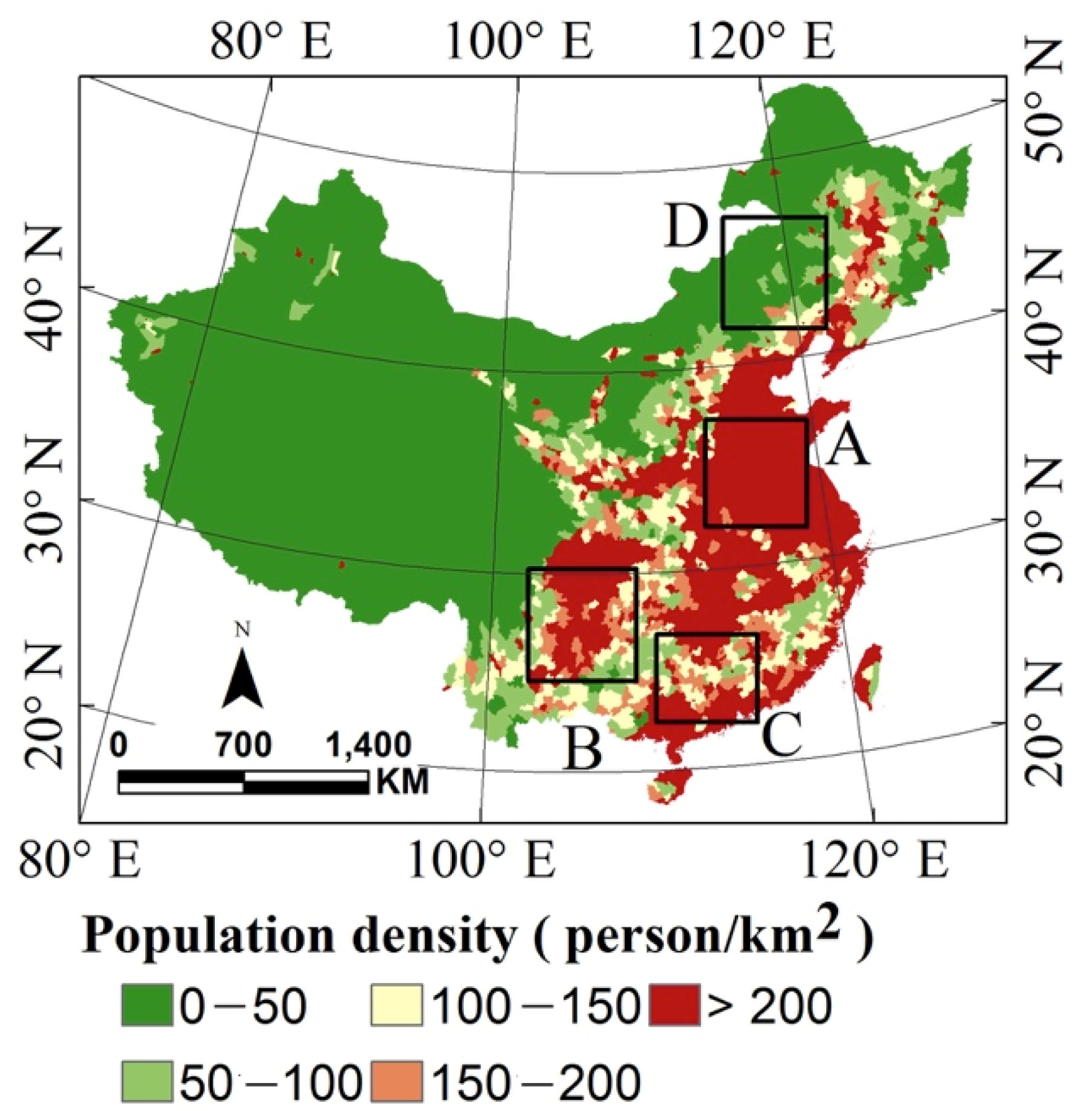
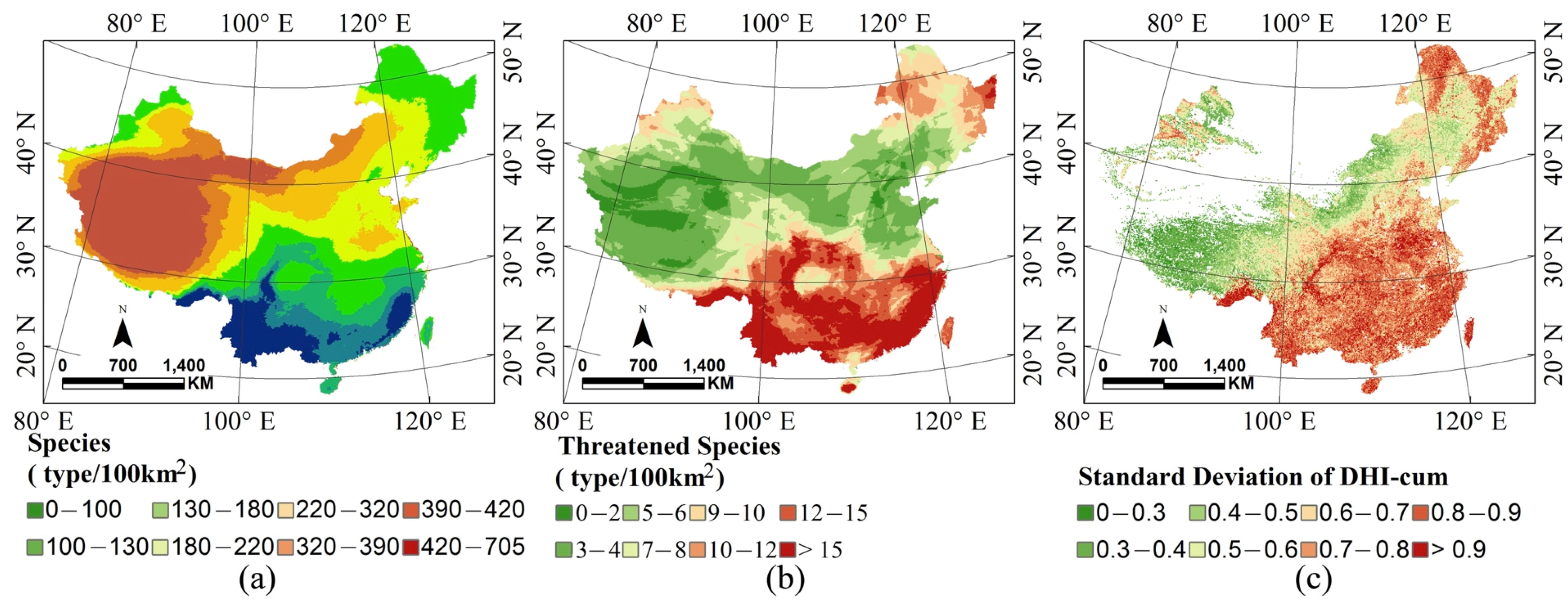
3.1. Ecological Setting

China (see Figure 2) is the third largest country (~9.6 million km²), extending over 37 (62) degrees of latitude (longitude), and the elevation ranges from −154 to 8844 m. It comprises climatically, topographically, and biologically complex areas [46]: five different climates cover China from the cold-temperate, temperate, warm-temperate, subtropical to the tropical regime. The highest mountain range is the “Third Pole” or Tibetan Plateau in western China, from where several major rivers of Asia originate, such as Mekong, Brahmaputra, Yangtze and Yellow rivers [47,48]. Species richness in China contributes about one-eighth of all species on Earth [49]. Now, applying the tools introduced in the previous section provides further information [50] on productivity and species richness and the changes and trends of biodiversity in China (see also [51,52]).

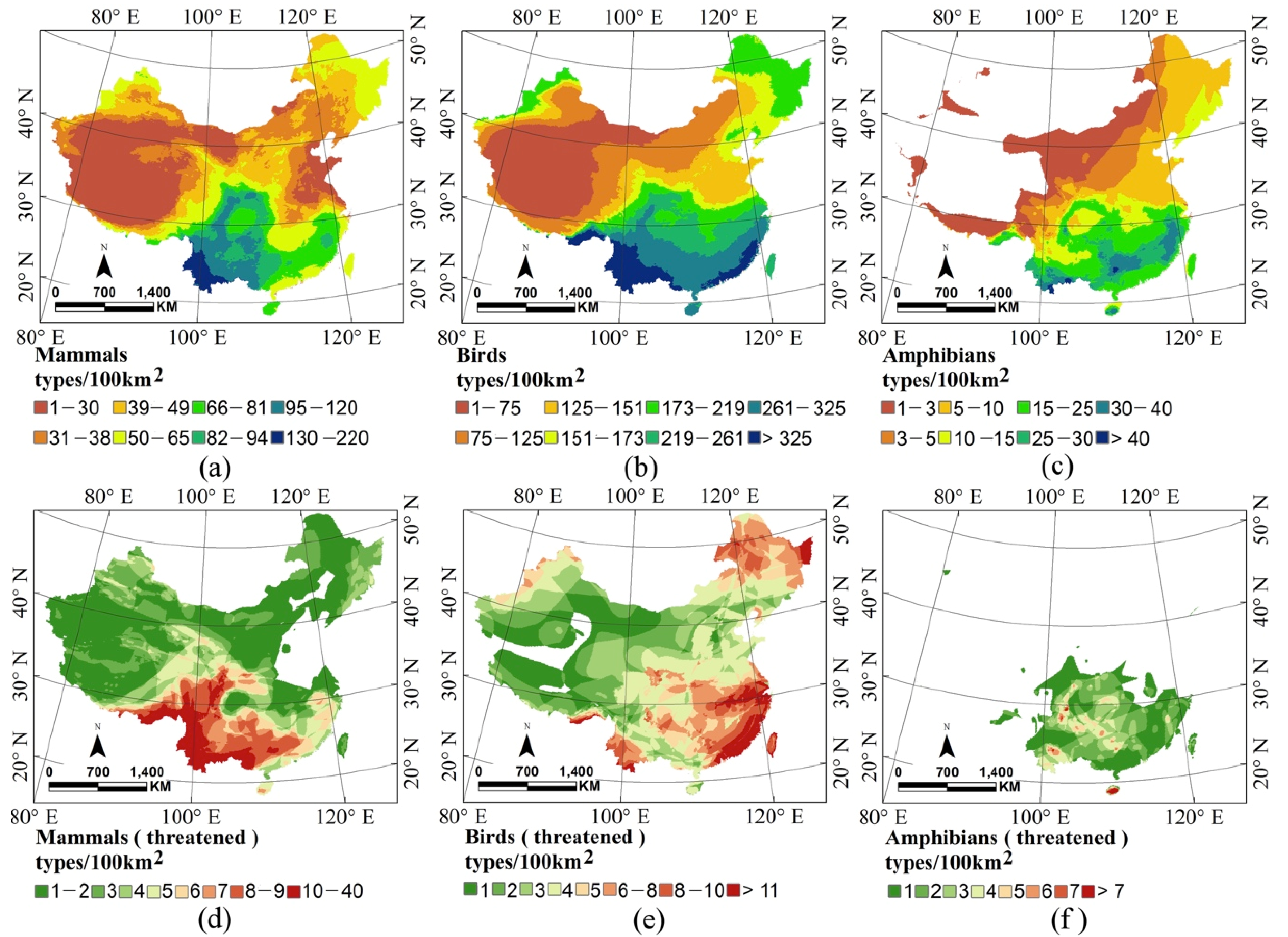
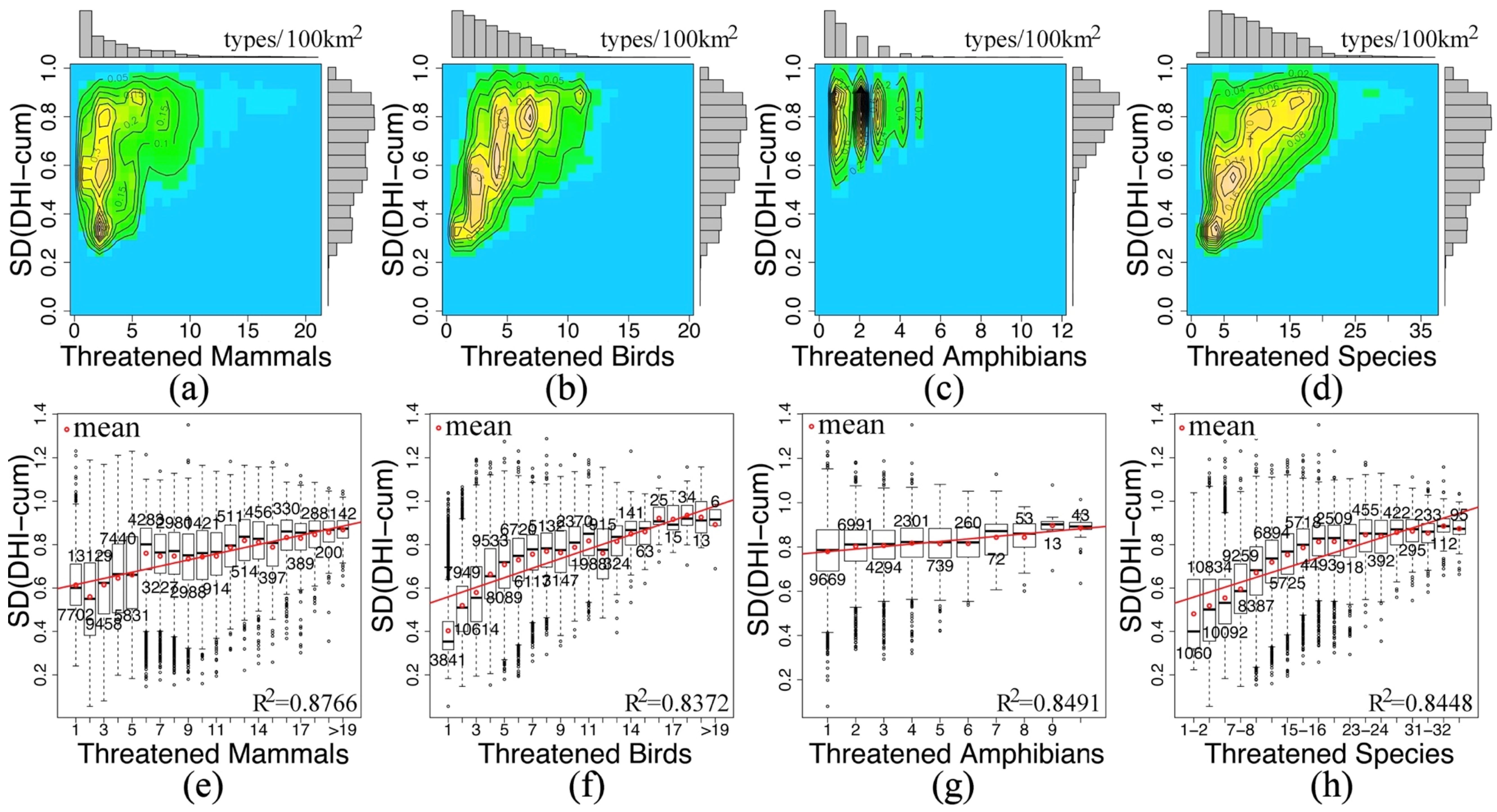
3.2. Remote Sensing Surrogates for Species and Threatened Species Richness

First, geographical distributions of field survey-based species richness are shown (in Figure 1), which, including mammals, birds and amphibians, are the focus in this study. To target biodiversity monitoring strategies for China, we apply remote sensing based DHI statistics (first and second moments, and trends) to China to serve as surrogates for species richness and threatened species richness. That is, to provide biodiversity classification in large areas, temporal measures of tendencies and variability are tested with actual field survey information (Figure 3 and Figure 4).

Frequency distribution and box plot based statistics are presented to relate richness of species and threatened species from field survey and decadal averaged Cumulative Productivity DHI-$\overline{cum}$ (and inter-annual standard deviation of DHI-$cum$). Figure 3 and Figure 4 show a linear relationship using the mean value of each actual field survey interval for mammals, birds, amphibians individually, and sum of three, with high correlation R² ~ 0.86 (R² ~ 0.85, for more details see

Table 1. The correlation coefficients between field survey species richness and remote sensing based DHI-$\overline{cum}$ using the simple linear regression.

Species Richness	Slopes	R2	p Value	DF	Pixels
Mammals	0.4516	0.8538	5.34e-07	13	64817
Birds	0.7980	0.9289	1.125e-06	9	64803
Amphibians	0.5586	0.8124	0.0002	8	56219
ALL	0.5393	0.8611	1.062e-06	12	71380

and

Table 2. The correlation coefficients between field survey based threatened species richness and the standard deviation of DHI-cum using the simple linear regression.

Threatened Species	Slopes	R2	p Value	DF	Pixels
Mammals	0.0142	0.8766	7.989e-10	18	62598
Birds	0.0220	0.8372	9.895e-09	18	67034
Amphibians	0.0115	0.8491	9.364e-05	8	24433
ALL	0.0227	0.8448	4.367e-08	16	67891

). This linear relationship supports the assumption that DHI components constitute surrogates of species richness and threatened species richness, at least for mammals, birds, and amphibians in China. The geographical distribution of remote sensing and field survey data are displayed in Figure 5 and the following results are noted:

(1) Productivity and species richness are positively correlated with areas of high productivity supporting a relatively high level of species richness [54,55,56,57,58,59]. Remote sensing based productivity, more specifically DHI-cum shows a linear relationship with estimated species richness. Lack of vegetation productivity, or DHI-cum, limits the species spatial distribution due to restricted food resources and habitat.

(2) Similarly, remote sensing based variability of land surface productivity, SD(DHI-cum), shows a linear relationship with estimates of endangered species richness. In addition, variability of land surface productivity occurs in regions with relatively high species richness. As regions with high species richness are more resilient, they recover from perturbations [60] and thus provide a relatively stable environment for their biomes and vice versa.

(3) Species richness and human population density in China tend to concentrate in regions with high species richness, which decreases from the Southeast towards the Northwest. The potential species richness and human population density are positively correlated (see Figure 2 and Figure 6a), because both respond positively to increasing levels of primary productivity [61].

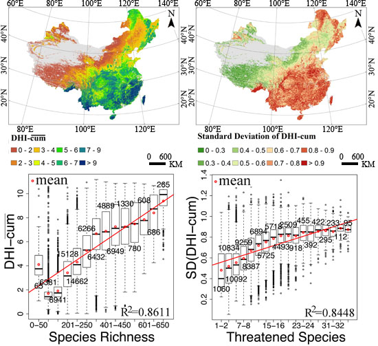
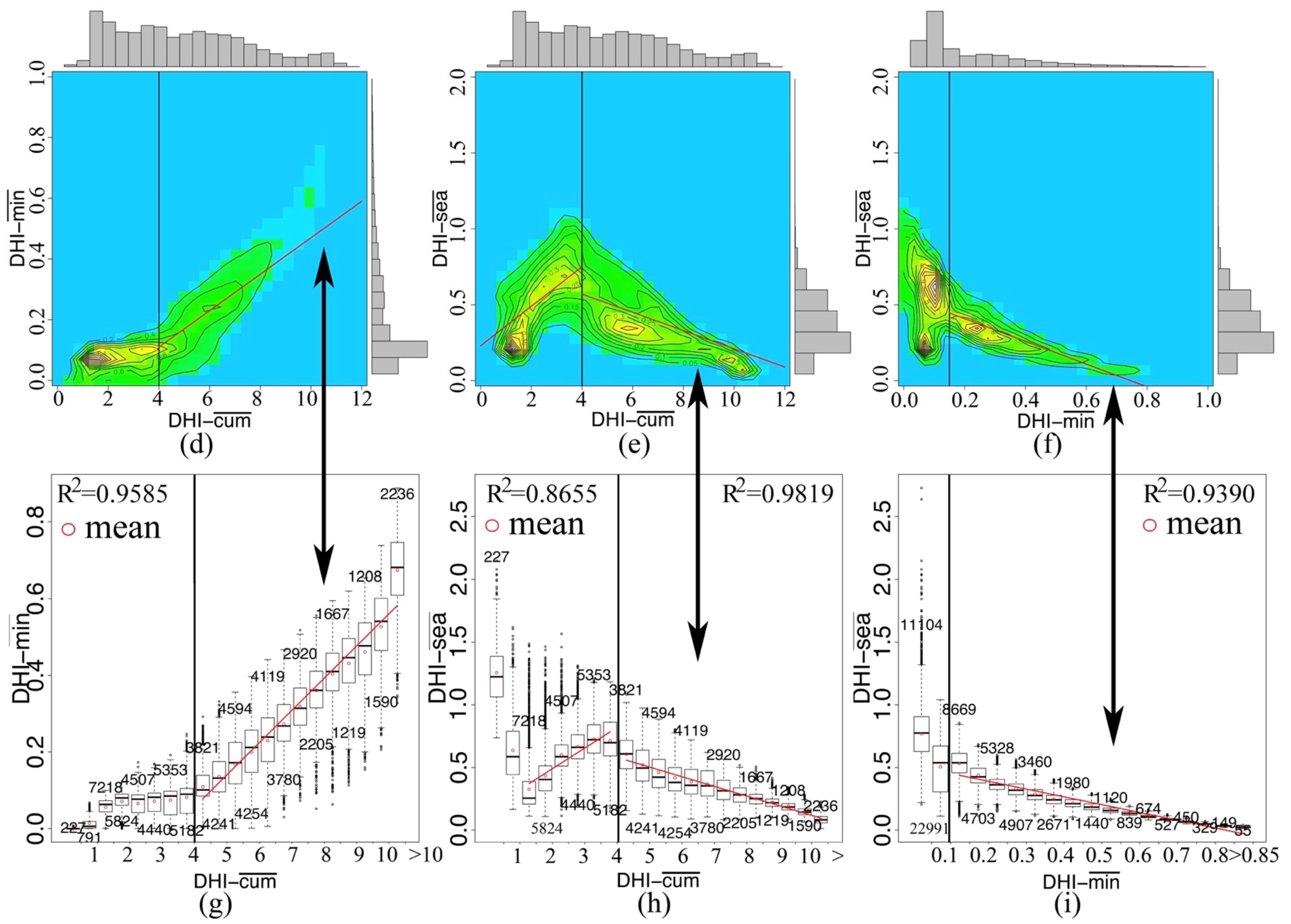
3.3. Dynamic Habitat Analysis in China

The linear relationship obtained in the previous section provides the underpinning of the subsequent dynamic habitat analysis. The geographical distributions of DHI-($\overline{cum},\overline{min},\overline{sea}$) components are displayed in Figure 6a–c:

(1) DHI-($\overline{cum},\overline{min}$) decrease from the warm and wet Southeast to the cold and arid Northwest, except for the mixed forest cover of the Greater and Lesser Khingan Mountains [62] and for the rainforest covered low-altitude regions on the Tibetan Plateau in the Shannan and Linzhi Prefectures [63].

(2) Megacities in eastern China (latitude 30 to 40°N) could not be distinguished from planted regions in the Northwest Plain when analyzing DHI-$\overline{cum}$ only (see light green regions). But DHI-$\overline{min}$ shows an obvious change (that is, a decrease, as confirmed by the scattered brown regions) separating megacities from planted regions and leaving only evergreen biomes at high values (dark green).

(3) DHI-$\overline{sea}$ associated with DHI-$\overline{cum}$, show low value is low in regions characterized by both high (southern evergreen forest regions) and low (northwestern sparsely vegetated regions) cumulative productivity. Furthermore, DHI-$\overline{sea}$ is positively related to the number of cropping times per year (Northeast > North > South China). For example, a relatively short growing season (May to September) and low winter temperature (−24 to −9 °C in January) in northeastern China allows only one crop per year [64,65,66,67]. But two crops per year occur in the North China Plain (−5 to 0 °C in January) governed by a long growing season from March to September [66,68,69]. Furthermore, South China has a longer growing season (February to December) and higher winter temperatures (0 to 16 °C in January) which allow two or three crops per year [70].

Frequency distributions (Figure 6d–i) allow a comparison of all DHI components:

(1) DHI-$\overline{cum}$~4 separates the relationship with DHI-($\overline{min}$, $\overline{sea}$). DHI-$\overline{min}$ (or $\overline{sea}$) is independent of (or positively related to) DHI-$\overline{cum}$ where DHI-$\overline{cum}$< ~4 but positively (or negatively) related where DHI-$\overline{cum}$ > ~4. The change from low to high DHI-$\overline{cum}$ follows the direction from the Northwest (red) to the Southeast (dark green, see Figure 6a). Exceptions are the first two bins in Figure 6h with 3.04% (227 + 791) pixels appear to be not aligned with the trend. Due to the small number and the discrete distribution, no exceptions appear in the zero lines of the density plot (Figure 6e).

(2) Likewise, DHI-$\overline{min}$~0.1 separates the relationship with DHI-$\overline{sea}$. DHI-$\overline{sea}$ is independent where DHI-$\overline{min}$ < ~0.1 but negatively related where DHI-$\overline{min}$ > ~0.1. The change from low to high of DHI-$\overline{min}$ is also from the Northwest (red) to the Southeast (dark green, see Figure 6b).

(3) The DHI-$\overline{cum}$ increase is related to vegetation types changing from grass to deciduous forest and to evergreen forest. Low DHI-$\overline{min}$ < ~0.1 corresponds to a wide range of DHI-$\overline{sea}$ in the geographically less-vegetated Tibetan Plateau and widespread cropped Northeast Plain (Figure 6b–c).

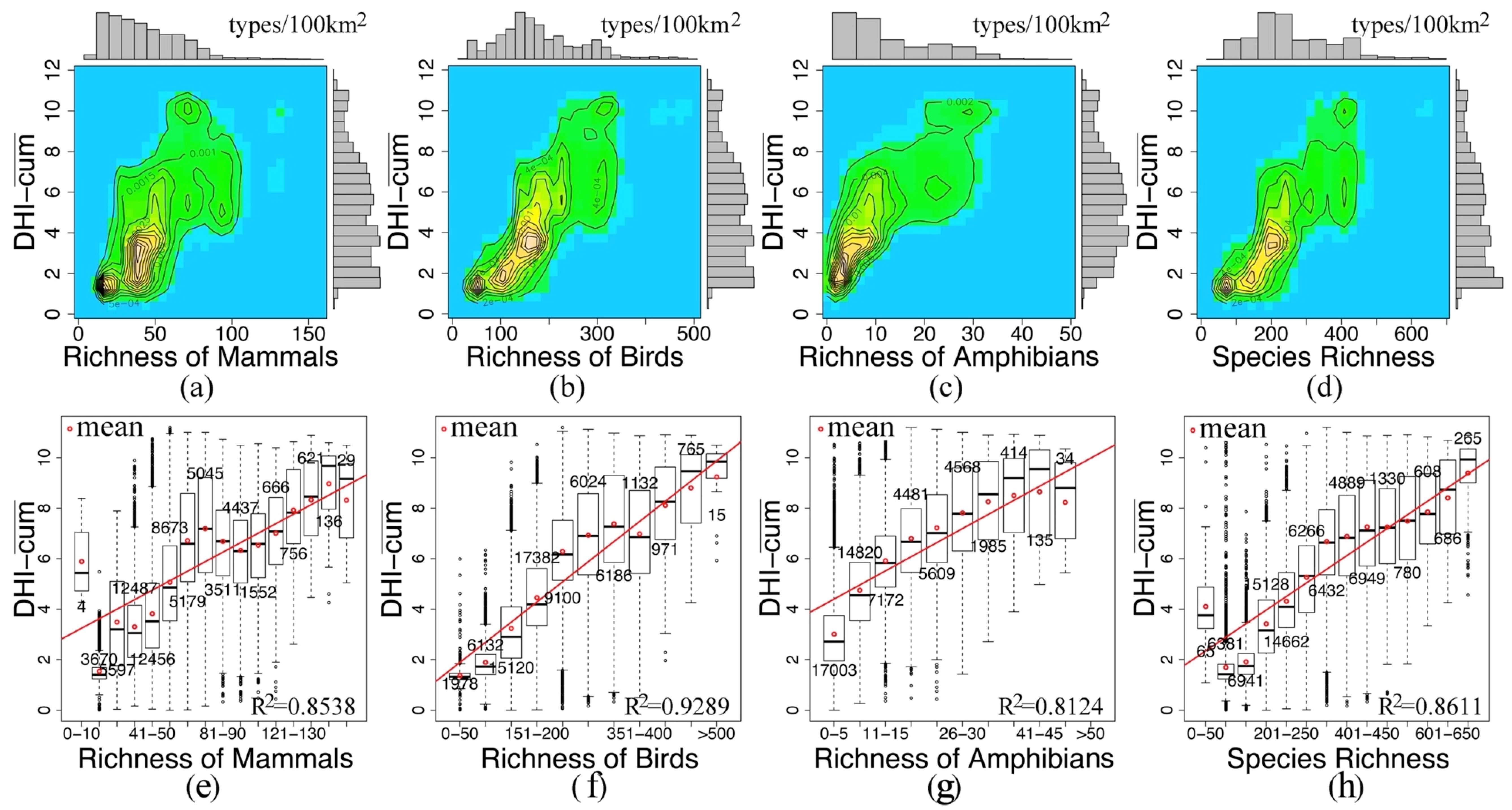
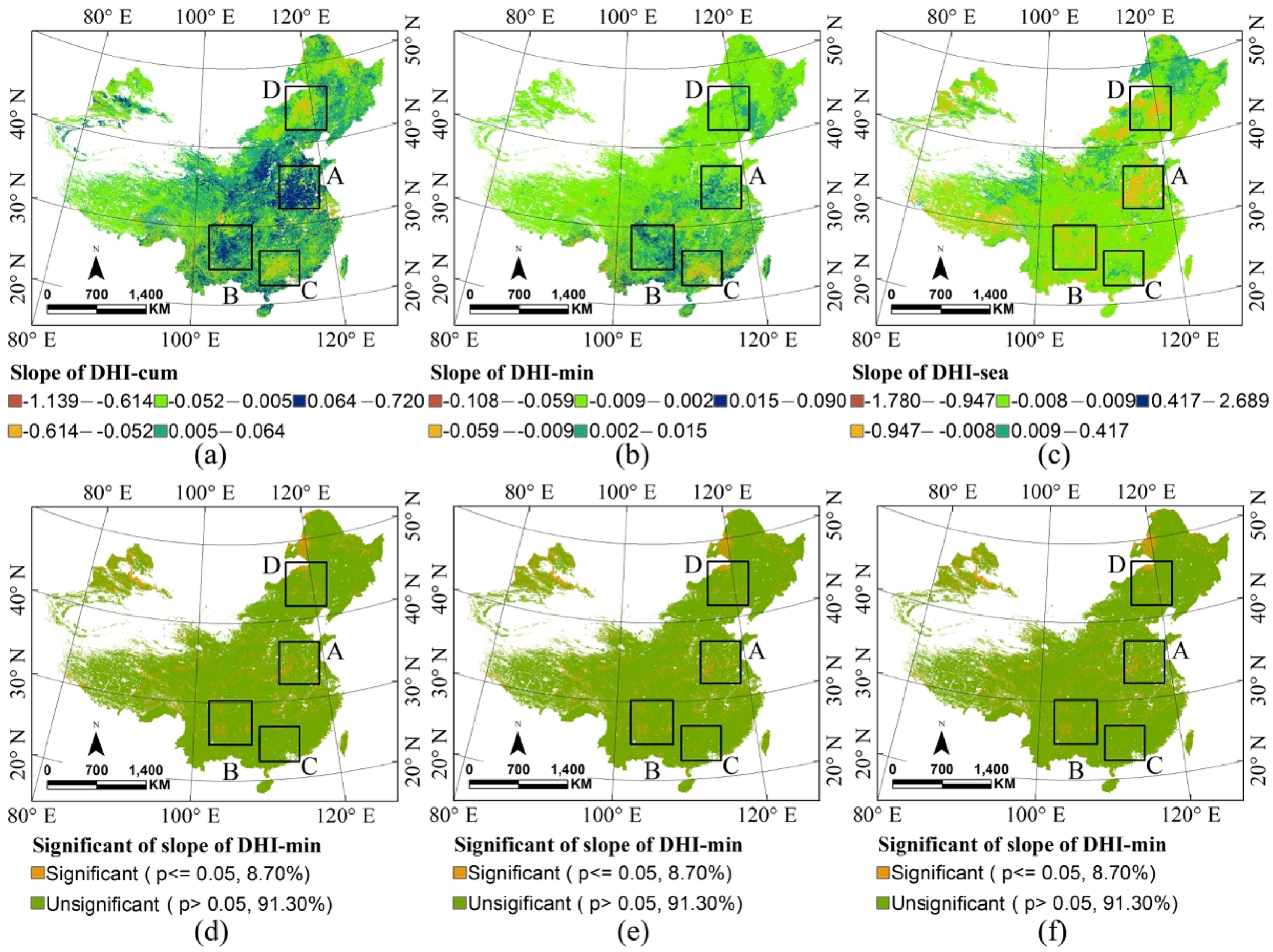
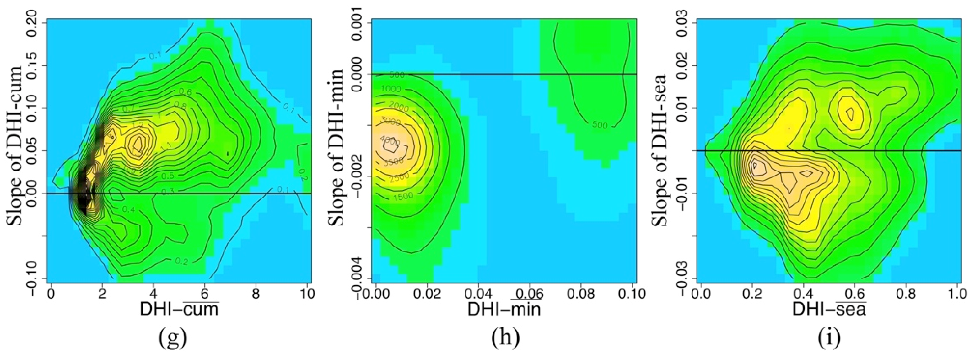
3.4. Regression and Change

Linear regression analyses applied to the long-term (2001–2010) DHI-(cum,min,sea) components are displayed geographically in Figure 7a–f including slope and significance (see also

Table 3. Significance of slope of Dynamic Habitat Index components: Cumulative Annual Productivity DHI-cum, Minimum Annual Apparent Cover DHI-min and Seasonal Variation of Greenness DHI-sea.

Significant	Slope of DHI-cum	Slope of DHI-min	Slope of DHI-sea
p ≤ 0.05	15.76%	8.70%	9.85%
p > 0.05	84.24%	91.30%	90.15%

). Four sub-regions, North China Plain, Nanling Mountains, Yunnan–Guizhou Plateau, and eastern Inner Mongolia, are highlighted due to the strong tendencies of the three DHI components, as well as the regional differences of climate, population density, species and endangered species richness. The following results are noted:

(1) The maximum slopes of decreasing DHI-sea and increasing DHI-(cum,min) occur in the cropland dominated (cropland accounts for 78.25%) North China Plain (Frame A), which is related to increasing temperatures in winter [71] and the so-called agricultural double-delay technology [69] delaying both the harvesting of maize and the sowing of wheat by about seven days.

(2) These phenomena are also observed in the Yunnan–Guizhou Plateau (Frame B) due to the implementation of China’s National Forest Conservation Program since 2000. Reforestation in Yunnan-Guizhou Plateau has shown forest coverage increasing from 40.77% (23.83%) in 1999 to 47.50% (31.61%) in 2008 [72].

(3) In contrast, the spatial–temporal distribution of the slope of DHI-sea can be associated with extreme climate events, varying from the well-vegetated south to less-vegetated north: the maximum increasing (decreasing) slopes of DHI-sea (cum,min) occur in Nanling Mountains (Frame C), where an ice storm occurred in 2008 [73,74]. The maximum slope decrease (decrease) of DHI-sea (cum,min) occurs in Inner-Mongolia (Frame D) perhaps due to a decline of accumulated precipitation over northern China during the summer season of 2009 [75].

Comparison between the three DHI components and their relationship tendencies lead, for most regions of significant change, to the following results (Figure 7g–i): (1) Significant slopes of DHI-cum, DHI-min, and DHI-sea occur in 15.76%, 8.70% and 9.85% of the total area, respectively. (2) DHI-cum tendencies increase if their values are high. (3) The slopes of DHI-(min,sea) decrease (increase) if their values are low (high), which is related to the bi-modality of the distribution separating DHI-$\overline{min}$ (DHI-$\overline{sea}$) near 0.05 (0.5).

4. Conclusions

In summarizing, although DHI is not a new index and its usefulness has been tested using actual biodiversity data in Australia, Canada and North America, we have, for the first time, applied this index in China. Assuming that DHI constitutes a viable surrogate of species richness without testing any relationship with actual species richness may be incorrect and could be misleading when extending the analysis to endangered species richness. Therefore, we first used field survey-based species richness data to test MODIS-based DHI for its applicability in China employing the DHI linear relationship. Similarly, we use field survey-based endangered species richness data to test MODIS-based standard deviation of DHI, while also using their respective linear relationships. Note that estimating the uncertainty of listed species as “potential” compared to actual species is an important issue for practical application on the regional scale (Guest Editor’s personal communication) but beyond the scope of this analysis. Here, the remote sensing derived statistic of annual productivity (i.e. first and second moments) is the only attributor used for estimating species and endangered species richness. Variables characterizing external climate and internal anthropogenic impact also contribute to the biodiversity dynamics as well [50,58,76,77]; for details in an ecohydrological, framework see Cai et al. [51,52] and Fraedrich et al. [78].

Geographic distributions of the species and threatened species census (2013, types/10 × 10 km²) of mammals, amphibians and birds are globally available, which thus makes our approach applicable for other continents or on a global scale. Furthermore, a large number of processes or events can cause biodiversity change which, for sake of simplicity, can be categorized roughly as either abrupt or gradual. Abrupt changes are generally referred to as disturbances, including wildfires, high winds, landslides, floods, avalanches and alike. Taking long term means (decadal averaged DHI-$\overline{cum}$) and a dynamic metric (standard deviation of inter-annual DHI-cum) to compare them with static metrics (field surveys based species and endangered species richness) may lead to temporal mismatching, particularly when spatial resolution is high and abrupt changes occur frequently. The linear regression comparisons do not exclude the identification of abrupt biodiversity changes or the distinction between subsequent time series, which can be very important for the interpretation of biodiversity processes. Gradual biodiversity change comprises an ecological succession, and these successional processes are subject to many variables that may or may not lead to some static or final state, and they set limits on the predictability of future living conditions of individual species.

This analysis is focused on China as the study region, which, consisting of 71,380 pixels with 10 × 10 km² spatial resolution, allows the following estimates of the underlying dynamics of species distribution and abundance, the adequate level of resources, and the pressure on biomes from the external environment.

(1) The decadal mean Cumulative Annual Productivity, DHI-$\overline{cum}$ < 4, in Northwest China (DHI-$\overline{cum}$ > 4 in Southeast China) shows a stable (positive) relation with the Minimum Annual Apparent Cover DHI-$\overline{min}$~0.1 and is positively (negatively) related to Seasonal Variation of Greenness DHI-$\overline{sea}$.

(2) The significant decadal tendencies reveal bimodal frequency distributions aligned near DHI-min~0.05 and DHI-sea~0.5 separated by zero slopes; that is, regions with small DHI-min (and DHI-sea) values are becoming smaller (and smaller), and regions with high DHI-min (and DHI-sea) are becoming higher (and higher).

(3) Land surface vegetation productivity and its variability have an effective impact on the richness of species and threatened species. Areas with high productivity support a relatively high level of species richness, and threatened species richness increases in frequently varied productivity regions. The restricted food resources and habitat, which lead to a reduced vegetation productivity, confine the species’ spatial distributions and also the human population density.

(4) For conservation planning, regions with high variability require more attention due to the high positive relationships with threatened species richness. Therefore, monitoring spatial-temporal dynamics of China’s terrestrial species and threatened species richness (by first/second moments and tendencies of remote sensing based DHI) may also provide the data necessary to support decision making processes.

These results promote our current understanding of the spatial-temporal dynamics of China’s terrestrial biodiversity, especially of effects induced by climate and anthropogenic changes on habitat dynamics based biome accumulation, minimum coverage and vegetation seasonality. Areas with anthropogenic activities, including cropping and reforestation contribute mainly to the DHI components changing in the North China Plain and Yunnan-Guizhou Plateau. Impacts by climate extremes, such as severe droughts and or ice storms, are detected in the Nanling Mountain and Inner Mongolia. In conclusion, this research contributes to a remote sensing based method to support the planning of natural resources conservation, and in turn, to protect biodiversity.

References

1. Koh, L.P.; Dunn, R.R.; Sodhi, N.S.; Colwell, R.K.; Proctor, H.C.; Smith, V.S. Species coextinctions and the biodiversity crisis. Science 2004, 305, 1632–1634. [Google Scholar] [CrossRef] [PubMed]
2. Dirzo, R.; Raven, P.H. Global state of biodiversity and loss. Ann. Rev. Environ. Resour. 2003, 28, 137–167. [Google Scholar] [CrossRef]
3. Ehrlich, P.R.; Daily, G.C. Population extinction and saving biodiversity. Ambio 1993, 22, 64–68. [Google Scholar]
4. Hughes, J.B.; Daily, G.C.; Ehrlich, P.R. Population diversity: Its extent and extinction. Science 1997, 278, 689–692. [Google Scholar] [CrossRef] [PubMed]
5. May, R.M.; Tregonning, K. Global conservation and UK government policy. In Conservation in a Changing World; Cambridge University Press: London, UK, 1998; pp. 287–301. [Google Scholar]
6. Daily, G. Nature’s Services: Societal Dependence on Natural Ecosystems; Island Press: Washington, DC, USA, 1997. [Google Scholar]
7. Larigauderie, A.; Prieur-Richard, A.-H.; Mace, G.M.; Lonsdale, M.; Mooney, H.A.; Brussaard, L.; Cooper, D.; Cramer, W.; Daszak, P.; Díaz, S. Biodiversity and ecosystem services science for a sustainable planet: The diversitas vision for 2012–2020. Curr. Opin. Environ. Sust. 2012, 4, 101–105. [Google Scholar] [CrossRef] [PubMed]
8. Rohlf, D.J. Six biological reasons why the endangered species act doesn’t work—And what to do about it. Conserv. Biol. 1991, 5, 273–282. [Google Scholar] [CrossRef]
9. Telford, L. Update on endangered species protection in Canada. Endanger. Spec. Update 2000, 94–99. [Google Scholar]
10. Zhang, P.; Shao, G.; Zhao, G.; Le Master, D.C.; Parker, G.R.; Dunning, J.B.; Li, Q. China’s forest policy for the 21st century. Science 2000, 288, 2135–2136. [Google Scholar] [CrossRef] [PubMed]
11. Uchida, E.; Xu, J.; Rozelle, S. Grain for green: Cost-effectiveness and sustainability of China’s conservation set-aside program. Land Econ. 2005, 81, 247–264. [Google Scholar] [CrossRef]
12. Xu, W.; Ouyang, Z.; Viña, A.; Zheng, H.; Liu, J.; Xiao, Y. Designing a conservation plan for protecting the habitat for giant pandas in the Qionglai mountain range, China. Divers. Distrib. 2006, 12, 610–619. [Google Scholar] [CrossRef]
13. Gong, M.; Yu, C. Study on the Corridors of Giant Panda; China Forestry Publishing House: Beijing, China, 2003. [Google Scholar]
14. Zhu, C.; Feng, G. A Case Study on China’s Policy of Converting Steep Cultivated Land to Forest or Grassland; China’s Forestry Press: Beijing, China, 2002. [Google Scholar]
15. Slavin, R.E. Best evidence synthesis: An intelligent alternative to meta-analysis. J. Clin. Epidemiol. 1995, 48, 9–18. [Google Scholar] [CrossRef]
16. Kerr, J.T.; Southwood, T.; Cihlar, J. Remotely sensed habitat diversity predicts butterfly species richness and community similarity in Canada. Proc. Nat. Acad. Sci. USA 2001, 98, 11365–11370. [Google Scholar] [CrossRef] [PubMed]
17. Livingston, M.; Shaw, W.W.; Harris, L.K. A model for assessing wildlife habitats in urban landscapes of eastern Pima county, Arizona (USA). Landsc. Urban Plann. 2003, 64, 131–144. [Google Scholar] [CrossRef]
18. Pauleit, S.; Ennos, R.; Golding, Y. Modeling the environmental impacts of urban land use and land cover change—A study in Merseyside, UK. Landsc. Urban Plann. 2005, 71, 295–310. [Google Scholar] [CrossRef]
19. Turner, W.; Spector, S.; Gardiner, N.; Fladeland, M.; Sterling, E.; Steininger, M. Remote sensing for biodiversity science and conservation. Trends Ecol. Evol. 2003, 18, 306–314. [Google Scholar] [CrossRef]
20. Coops, N.C.; Wulder, M.A.; Duro, D.C.; Han, T.; Berry, S. The development of a Canadian dynamic habitat index using multi-temporal satellite estimates of canopy light absorbance. Ecol. Indic. 2008, 8, 754–766. [Google Scholar] [CrossRef]
21. Mackey, B.G.; Bryan, J.; Randall, L. Australia’s dynamic habitat template 2003. In Proceedings of the MODIS Vegetation Workshop II, Missoula, MT, American, 17 April 2004.
22. Michaud, J.-S.; Coops, N.C.; Andrew, M.E.; Wulder, M.A. Characterising spatiotemporal environmental and natural variation using a dynamic habitat index throughout the province of Ontario. Ecol. Indic. 2012, 18, 303–311. [Google Scholar] [CrossRef]
23. Whittaker, R.J. Meta-analyses and mega-mistakes: Calling time on meta-analysis of the species richness-productivity relationship. Ecology 2010, 91, 2522–2533. [Google Scholar] [CrossRef] [PubMed]
24. Duro, D.C.; Coops, N.C.; Wulder, M.A.; Han, T. Development of a large area biodiversity monitoring system driven by remote sensing. Prog. Phys. Geog. 2007, 31, 235–260. [Google Scholar] [CrossRef]
25. Fritz, S.; McCallum, I.; Schill, C.; Perger, C.; See, L.; Schepaschenko, D.; van der Velde, M.; Kraxner, F.; Obersteiner, M. Geo-wiki: An online platform for improving global land cover. Environ. Modell. Softw. 2012, 31, 110–123. [Google Scholar] [CrossRef]
26. Fritz, S.; See, L.; McCallum, I.; You, L.; Bun, A.; Moltchanova, E.; Duerauer, M.; Albrecht, F.; Schill, C.; Perger, C. Mapping global cropland and field size. Glob. Change Biol. 2015, 21, 1980–1992. [Google Scholar] [CrossRef] [PubMed] [Green Version]
27. See, L.; McCallum, I.; Fritz, S.; Perger, C.; Kraxner, F.; Obersteiner, M.; Baruah, U.D.; Mili, N.; Kalita, N.R. Mapping cropland in Ethiopia using crowdsourcing. Int. J. Geosci. 2013, 4, 6–13. [Google Scholar] [CrossRef]
28. Berry, S.; Mackey, B.; Brown, T. Potential applications of remotely sensed vegetation greenness to habitat analysis and the conservation of dispersive fauna. Pac. Cons. Biol. 2007, 13, 120–127. [Google Scholar]
29. Coops, N.C.; Fontana, F.M.A.; Harvey, G.K.A.; Nelson, T.A.; Wulder, M.A. Monitoring of a national-scale indirect indicator of biodiversity using a long time-series of remotely sensed imagery. Can. J. Remote Sens. 2014, 40, 179–191. [Google Scholar] [CrossRef]
30. Coops, N.C.; Wulder, M.A.; Iwanicka, D. Demonstration of a satellite-based index to monitor habitat at continental-scales. Ecol. Indic. 2009, 9, 948–958. [Google Scholar] [CrossRef]
31. Coops, N.C.; Waring, R.H.; Wulder, M.A.; Pidgeon, A.M.; Radeloff, V.C. Bird diversity: A predictable function of satellite-derived estimates of seasonal variation in canopy light absorbance across the United States. J. Biogeogr. 2009, 36, 905–918. [Google Scholar] [CrossRef]
32. Holmes, K.R.; Nelson, T.A.; Coops, N.C.; Wulder, M.A. Biodiversity indicators show climate change will alter vegetation in parks and protected areas. Diversity 2013, 5, 352–373. [Google Scholar] [CrossRef]
33. Andrew, M.E.; Wulder, M.A.; Coops, N.C.; Baillargeon, G. Beta-diversity gradients of butterflies along productivity axes. Glob. Ecol. Biogeogr. 2012, 21, 352–364. [Google Scholar] [CrossRef]
34. Tian, Y.; Zhang, Y.; Knyazikhin, Y.; Myneni, R.B.; Glassy, J.M.; Dedieu, G.; Running, S.W. Prototyping of MODIS LAI and fPAR algorithm with LASUR and Landsat data. IEEE Trans. Geosci. Remote Sens. 2000, 38, 2387–2401. [Google Scholar] [CrossRef]
35. Jenkins, C.N.; Pimm, S.L.; Joppa, L.N. Global patterns of terrestrial vertebrate diversity and conservation. PNAS 2013, 110, 2602–2610. [Google Scholar] [CrossRef] [PubMed]
36. Pimm, S.L.; Jenkins, C.N.; Abell, R.; Brooks, T.M.; Gittleman, J.L.; Joppa, L.N.; Raven, P.H.; Roberts, C.M.; Sexton, J.O. The biodiversity of species and their rates of extinction, distribution, and protection. Science 2014, 344, 987–997. [Google Scholar] [CrossRef] [PubMed]
37. Mapping the World’s Biodiversity. Available online: http://www.biodiversitymapping.org (accessed on 10 November 2014).
38. Evans, K.L.; Warren, P.H.; Gaston, K.J. Species–energy relationships at the macroecological scale: A review of the mechanisms. Biol. Rev. 2005, 80, 1–25. [Google Scholar] [CrossRef] [PubMed]
39. Skidmore, A.K.; Oindo, B.O.; Said, M.Y. Biodiversity assessment by remote sensing. In Proceedings of the 30th International Symposium on Remote Sensing of the Environment: Information for Risk Management and Sustainable Development, Honolulu, HI, USA; 2003. [Google Scholar]
40. Schwartz, C.C.; Haroldson, M.A.; White, G.C.; Harris, R.B.; Cherry, S.; Keating, K.A.; Moody, D.; Servheen, C. Temporal, spatial, and environmental influences on the demographics of grizzly bears in the greater Yellowstone ecosystem. Wildlife Monogr. 2006, 161, 1–8. [Google Scholar] [CrossRef]
41. Gilmore, S.; Mackey, B.; Berry, S. The extent of dispersive movement behaviour in Australian vertebrate animals, possible causes, and some implications for conservation. Pac. Cons. Biol. 2007, 13, 93–103. [Google Scholar]
42. McLoughlin, P.D.; Wal, E.V.; Lowe, S.J.; Patterson, B.R.; Murray, D.L. Seasonal shifts in habitat selection of a large herbivore and the influence of human activity. Basic Appl. Ecol. 2011, 12, 654–663. [Google Scholar] [CrossRef]
43. Holben, B.N. Characteristics of maximum-value composite images from temporal AVHRR data. Int. J. Remote Sens. 1986, 7, 1417–1434. [Google Scholar] [CrossRef]
44. Rao, C.R.; Toutenburg, H.; Shalabh, H.C.; Schomaker, M. Linear Models and Generalizations. Least Squares and Alternatives, 3rd ed.; Springer: New York, NY, USA, 2008. [Google Scholar]
45. Mamtimin, B.; Et-Tantawi, A.M.M.; Schaefer, D.; Meixner, F.X.; Domroes, M. Recent trends of temperature change under hot and cold desert climates: Comparing the Sahara (Libya) and central Asia (Xinjiang, China). J. Arid. Environ. 2011, 75, 1105–1113. [Google Scholar] [CrossRef]
46. López-Pujol, J.; Zhang, F.-M.; Ge, S. Plant biodiversity in China: Richly varied, endangered, and in need of conservation. Biodivers Conserv. 2006, 15, 3983–4026. [Google Scholar] [CrossRef]
47. Cai, D.; Guan, Y.; Guo, S.; Zhang, C.; Fraedrich, K. Mapping plant functional types over broad mountainous regions: A hierarchical soft time-space classification applied to the Tibetan Plateau. Remote Sens. 2014, 6, 3511–3532. [Google Scholar] [CrossRef]
48. Yi, X.; Yin, Y.; Li, G.; Peng, J. Temperature variation in recent 50 years in the three-river headwaters region of Qinghai province. Acta Geogr. Sin. 2011, 66, 1451–1465. (In Chinese) [Google Scholar]
49. Harkness, J. Recent trends in forestry and conservation of biodiversity in China. China Q. 1998, 156, 911–934. (In Chinese) [Google Scholar] [CrossRef]
50. Nilsen, E.B.; Herfindal, I.; Linnell, J.D.C. Can intra-specific variation in carnivore home-range size be explained using remote-sensing estimates of environmental productivity? Ecoscience 2005, 12, 68–75. [Google Scholar] [CrossRef]
51. Cai, D.; Fraedrich, K.; Sielmann, F.; Guan, Y.; Guo, S.; Zhang, L.; Zhu, X. Climate and vegetation: An ERA-interim and GIMMS NDVI analysis. J. Clim. 2014, 27, 5111–5118. [Google Scholar] [CrossRef]
52. Cai, D.; Fraedrich, K.; Sielmann, F.; Zhang, L.; Zhu, X.; Guo, S.; Guan, Y. Vegetation dynamics on the Tibetan Plateau (1982 to 2006): An attribution by eco-hydrological diagnostics. J. Clim. 2015, 28, 4576–4584. [Google Scholar] [CrossRef]
53. National Bureau of Statistics of the People’s Republic of China. Available online: http://www.stats.gov.cn (accessed on 10 June 2013).
54. Jetz, W.; Fine, P.V.A. Global gradients in vertebrate diversity predicted by historical area-productivity dynamics and contemporary environment. PLoS Biol. 2012, 10, e1001292. [Google Scholar] [CrossRef] [PubMed]
55. Jetz, W.; Rahbek, C. Geographic range size and determinants of avian species richness. Science 2002, 297, 1548–1551. [Google Scholar] [CrossRef] [PubMed]
56. Qian, H.; Kissling, W.D. Spatial scale and cross-taxon congruence of terrestrial vertebrate and vascular plant species richness in China. Ecology 2010, 91, 1172–1183. [Google Scholar] [CrossRef] [PubMed]
57. Waide, R.B.; Willig, M.R.; Steiner, C.F.; Mittelbach, G.; Gough, L.; Dodson, S.I.; Juday, G.P.; Parmenter, R. The relationship between productivity and species richness. Annu. Rev. Ecol. Syst. 1999, 30, 257–300. [Google Scholar] [CrossRef]
58. Chase, J. Historical and contemporary factors govern global biodiversity patterns. PLoS Biol. 2012, 10, e1001294. [Google Scholar] [CrossRef] [PubMed]
59. Walker, R.E.; Stoms, D.M.; Estes, J.E.; Cayocca, K.D. Relationships between Biological Diversity and Multi-Temporal Vegetation Index Data in California; Soc Photogrammetry & Remote Sensing: Washington, DC, USA, 1992; pp. 562–571. [Google Scholar]
60. Moore, J.C.; De Ruiter, P.C.; Hunt, H.W. Influence of productivity on the stability of real and model ecosystems. Sci. New York Then Wash. 1993, 261, 906–908. [Google Scholar] [CrossRef] [PubMed]
61. Chown, S.L.; van Rensburg, B.J.; Gaston, K.J.; Rodrigues, A.S.L.; van Jaarsveld, A.S. Energy, species richness, and human population size: Conservation implications at a national scale. Ecol. Appl. 2003, 13, 1233–1241. [Google Scholar] [CrossRef] [Green Version]
62. Mao, D.; Wang, Z.; Luo, L.; Ren, C. Integrating AVHRR and MODIS data to monitor NDVI changes and their relationships with climatic parameters in Northeast China. Int. J. Appl. Earth Obs. 2012, 18, 528–536. [Google Scholar] [CrossRef]
63. Zhang, X.; Sun, S.; Zhou, Z.; Wang, R. Vegetation map of the People’s Republic of China (1:1,000,000); Geological Publishing House: Beijing, China, 2007. (In Chinese) [Google Scholar]
64. Chen, C.; Qian, C.; Deng, A.; Zhang, W. Progressive and active adaptations of cropping system to climate change in Northeast China. Eur. J. Agron. 2012, 38, 94–103. [Google Scholar] [CrossRef]
65. Liu, M.; Liu, G.H.; Wu, X.; Wang, H.; Chen, L. Vegetation traits and soil properties in response to utilization patterns of grassland in Hulun Buir city, Inner Mongolia, China. Chinese Geogr. Sci. 2014, 24, 471–478. [Google Scholar] [CrossRef]
66. Lu, A.; Kang, S.; Pang, D.; Wang, T.; Ge, J. Different landform effects on seasonal temperature patterns in China. Ecol. Envrion. 2008, 17, 1450–1452. [Google Scholar]
67. Wang, J.; Huang, J.; Yang, J. Overview of impacts of climate change and adaptation in China’s agriculture. J. Integr. Agric. 2014, 13, 1–17. [Google Scholar] [CrossRef]
68. Li, J.; Yu, Q.; Sun, X.; Tong, X.; Ren, C.; Wang, J.; Liu, E.; Zhu, Z.; Yu, G. Carbon dioxide exchange and the mechanism of environmental control in a farmland ecosystem in North China Plain. Sci. China Ser. D 2006, 49, 226–240. [Google Scholar] [CrossRef]
69. Mo, X.; Liu, S.; Lin, Z. Evaluation of an ecosystem model for a wheat–maize double cropping system over the North China plain. Environ. Modell. Softw. 2012, 32, 61–73. [Google Scholar] [CrossRef]
70. Song, Y.; Liu, B.; Zhong, H. Impact of global warming on the rice cultivable area in southern China in 1961–2009. Adv. Clim. Chang. Res. 2011, 7, 259–264. (In Chinese) [Google Scholar]
71. Wang, J.; Wang, E.; Yang, X.; Zhang, F.; Yin, H. Increased yield potential of wheat-maize cropping system in the North China Plain by climate change adaptation. Climat. Chang. 2012, 113, 825–840. [Google Scholar] [CrossRef]
72. Guo, Z. Study on Comprehensive Benefits Evaluation of Natural Forest Protection Program in Southwest China. Ph.D. Thesis, Beijing Forestry University, Beijing, China, 2011. [Google Scholar]
73. Huang, C.; Zhuang, X.; Li, R.; Liu, Z.; Jiang, B.; Zhai, C. Damaged status and early recovery of tree species in Wuzhishan of Nanling Mountains, South China after the ice storm in 2008. Chin. J. Ecol. 2012, 6, 1390–1396. (In Chinese) [Google Scholar]
74. Zhou, B.; Li, Z.; Wang, X.; Cao, Y.; An, Y.; Deng, Z.; Letu, G.; Wang, G.; Gu, L. Impact of the 2008 ice storm on moso bamboo plantations in Southeast China. J. Geophys. Res.: Biogeosci. 2011, 116, G00H06. [Google Scholar] [CrossRef]
75. Barriopedro, D.; Gouveia, C.M.; Trigo, R.M.; Wang, L. The 2009/10 drought in China: possible causes and impacts on vegetation. J. Hydrometeorol. 2012, 13, 1251–1267. [Google Scholar] [CrossRef]
76. Storch, D.; Davies, R.G.; Zajíček, S.; Orme, C.D.L.; Olson, V.; Thomas, G.H.; Ding, T.-S.; Rasmussen, P.C.; Ridgely, R.S.; Bennett, P.M.; et al. Energy, range dynamics and global species richness patterns: Reconciling mid-domain effects and environmental determinants of avian diversity. Ecol. Lett. 2006, 9, 1308–1320. [Google Scholar] [CrossRef] [PubMed]
77. Stein, A.; Gerstner, K.; Kreft, H. Environmental heterogeneity as a universal driver of species richness across taxa, biomes and spatial scales. Ecol. Lett. 2014, 17, 866–880. [Google Scholar] [CrossRef] [PubMed]
78. Fraedrich, K.F.; Sielmann, C.D.; Zhu, X. Climate dynamics on watershed scale: Along the rainfall-runoff chain. In The Fluid Dynamics of Climate, International Centre for Mechanical Sciences (CISM); Springer Verlag: Vienna, Austria, 2016; pp. 183–209. [Google Scholar]
Figure 1. Geographical distributions of field survey-based species richness of: (a) Mammals; (b) Birds; and (c) Amphibians. The threatened species richness of: (d) Mammals; (e) Birds; and (f) Amphibians (number of types per 100 km2, see [35,36]; downloadable from [37]). Due to a lack of data, marine islands were not considered.
Remotesensing 08 00227 g001
Figure 2. Geographical setting of China including the main land China, Hainan and Taiwan provinces: population census (2010) from National Bureau of Statistics of China (NBSC, downloadable from [53]) is introduced for interpretation (see Section 3.2). Four sub-regions are selected for the same purpose: A, North China Plain; B, Yunnan–Guizhou Plateau; C, Nanling Mountains; and D, eastern Inner Mongolia.
Remotesensing 08 00227 g002
Figure 3. Frequency distributions between field survey species richness and decadal averaged Cumulative Productivity DHI- cum ¯ are presented in (x,y)-format for: (a) (Mammals, DHI- cum ¯ ); (b) (Birds, DHI- cum ¯ ); (c) (Amphibians, DHI- cum ¯ ); and (d) (sum of three species, DHI- cum ¯ ). Boxplot based linear regression statistics of decadal averaged Cumulative Productivity DHI- cum ¯ versus field survey species richness of: (e) Mammals; (f) Birds; (g) Amphibians; and (h) sum of three species.
Remotesensing 08 00227 g003
Figure 4. Frequency distributions of the standard deviation of Annual Cumulative Productivity SD(DHI-cum) versus field survey based threatened species richness of: (a) Mammals; (b) Birds; (c) Amphibian; and (d) sum of three threatened species. Boxplot based linear regression statistics of the standard deviation of Annual Cumulative Productivity SD(DHI-cum) versus field survey of endangered species of: (e) Mammals; (f) Birds; (g) Amphibians; and (h) sum of three endangered species.
Remotesensing 08 00227 g004
Figure 5. Field survey based geographic distribution of: (a) species richness; (b) threatened species richness (sum of mammals, birds and amphibians from [37]); and (c) geographic distribution of remote sensing based standard deviation of Annual Cumulative Productivity SD(DHI-cum).
Remotesensing 08 00227 g005
Figure 6. Geographical distributions of climate mean of the dynamic habitat components (2001 to 2010): (a) Cumulative Annual Productivity, DHI- c u m ¯ ; (b) Minimum Annual Apparent Cover, DHI- m i n ¯ ; and (c) Seasonal Variation of Greenness, DHI- s e a ¯ . The interrelationships associated with frequency distributions in (x,y)-format are presented for: (d) DHI-( c u m ¯ ); (e) DHI-( c u m ¯ ); and (f) DHI-( m i n   ¯ ). The interrelation associated boxplots in (x,y)-format are presented in (x,y)-format for: (g) DHI-( c u m ¯ ); (h) DHI-( c u m ¯ ); and (i) DHI-( m i n   ¯ ).
Remotesensing 08 00227 g006aRemotesensing 08 00227 g006b
Figure 7. Geographical distribution of the ten-year linear regression trend of the dynamic habitat components (2001 to 2010): (a) Cumulative Annual Productivity DHI-cum; (b) Minimum Annual Apparent Cover DHI-min; and (c) Seasonal Variation of Greenness DHI-sea. The related significant distributions: (d) Cumulative Annual Productivity DHI-cum; (e) Minimum Annual Apparent Cover DHI-min; and (f) Seasonal Variation of Greenness DHI-sea. Temporal changes (tendencies) are presented in terms of frequency distributions in a (x,slope(x))-format for significant slope change regions with (g) DHI-cum, (h) DHI-min; (i) DHI-sea. Four sub-regions are selected: A, North China Plain; B, Yunnan-Guizhou Plateau; C, Nanling Mountains; and D, eastern Inner Mongolia.
Remotesensing 08 00227 g007aRemotesensing 08 00227 g007b