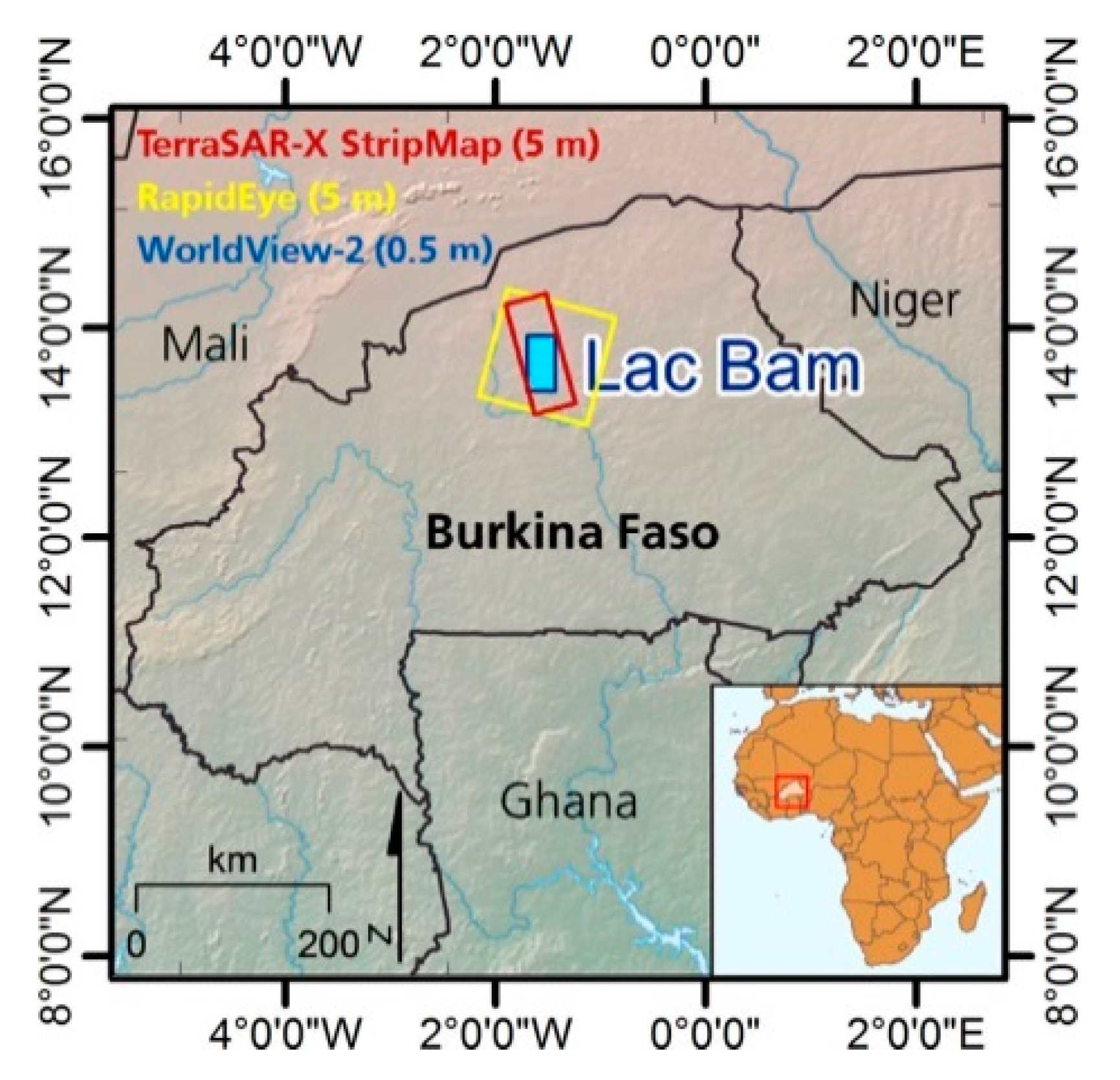
Article

Monitoring of the Lac Bam Wetland Extent Using Dual-Polarized X-Band SAR Data

German Aerospace Center (DLR), German Remote Sensing Data Center (DFD), Land Surface Department (LAX), Oberpfaffenhofen, Wessling 82234, Germany
*
Author to whom correspondence should be addressed.
Submission received: 23 December 2015 / Revised: 10 March 2016 / Accepted: 17 March 2016 / Published: 5 April 2016
(This article belongs to the Special Issue What can Remote Sensing Do for the Conservation of Wetlands?)

Abstract

:
Wetlands in semi-arid Africa are vital as water resource for local inhabitants and for biodiversity, but they are prone to strong seasonal fluctuations. Lac Bam is the largest natural freshwater lake in Burkina Faso, its water is mixed with patches of floating or flooded vegetation, and very turbid and sediment-rich. These characteristics as well as the usual cloud cover during the rainy season can limit the suitability of optical remote sensing data for monitoring purposes. This study demonstrates the applicability of weather-independent dual-polarimetric Synthetic Aperture Radar (SAR) data for the analysis of spatio-temporal wetland dynamics. A TerraSAR-X repeat-pass time series of dual-co-polarized HH-VV StripMap data—with intervals of 11 days, covering two years (2013–2015) from the rainy to the dry season—was processed to normalized Kennaugh elements and classified mono-temporally and multi-temporally. Land cover time series and seasonal duration maps were generated for the following four classes: open water, flooded/floating vegetation, irrigated cultivation, and land (non-wetland). The added value of dual-polarimetric SAR data is demonstrated by significantly higher multitemporal classification accuracies, where the overall accuracy (88.5%) exceeds the classification accuracy using single-polarimetric SAR intensity data (82.2%). For relevant change classes involving flooded vegetation and irrigated fields dual-polarimetric data (accuracies: 75%–97%) are favored to single-polarimetric data (42%–87%). This study contributes to a better understanding of the dynamics of semi-arid African wetlands in terms of water areas including water with flooded vegetation, and the location and timing of irrigated cultivations.

Graphical Abstract

1. Introduction

1.1. Remote Sensing of Wetlands in Semi-Arid Africa

Surface water located in water bodies, wetlands, and rivers is a critical resource in the semi-arid West-African Sahel. Regular monitoring of water sources is often only carried out at few selected wetlands or water bodies, and commonly applied as point-wise water level measurement. There is a lack of documentation of monitoring locations and measurements in many African countries. Major livelihood groups like farmers, pastoralists, and fishermen strongly depend on the existence and use of water, as does the local population and wildlife. From an ecological point of view, water bodies and wetlands are equally significant. They contain unique habitats, are of great importance for biodiversity, and provide a number of ecosystem services. The study area for this work is Lac Bam, which is located in the southern Sahel zone of Burkina Faso in West Africa. Significant areas of Lac Bam are covered by either floating or emergent flooded vegetation—resulting in areas of open water covered by macrophytes—or flooded grasses, shrubs, and trees [1]. As the largest freshwater lake in Burkina Faso, Lac Bam is of high importance for irrigated farming, animal watering, fishery, and extraction of water for drinking and sanitation purposes. The banks of the lake are increasingly used for irrigated agriculture—for which several motor pumps have been established [2]—and for animal watering, since the lake is located on a transhumant pastoralist route. Lac Bam is part of the global Ramsar List of Wetlands of International Importance, according to the intergovernmental Ramsar treaty [3]. Ramsar sites are selected according to their status as representative, rare, or unique wetland types, as well as on their fulfilment of some of the eight criteria of biological diversity defined by Ramsar [3]. Wetland conservation and restoration plays an important role for Lac Bam which has been degraded due to domestic use, farming, herding, and over-fishing, and suffers from increasing sedimentation and pollution [2,4,5].
Remote sensing-based wetland monitoring can be a challenging task because wetlands are often very dynamic—i.e., in terms of water area, water level, or vegetation presence and growth—especially in semi-arid areas with dedicated rainy and dry seasons. In addition, anthropogenically generated fluctuations due to water extraction for irrigated farming, domestic purposes, or power generation occur, coupled with water level regulation by man-made dams. Such dynamic environments require short temporal observation intervals, which is a key point of the study presented in this paper. The presence of different wetland or land cover class types on a small surface area requires the use of high spatial resolution data. Moreover, wetlands are very diverse, lack a unique land cover or vegetation type or feature, and also contain water below the Earth’s surface [6]. Ground measurements are only capable to provide local, point-wise information. This data can be provided with either a high temporal resolution (e.g., water gauge) or a large spatial coverage (e.g., ground-based mapping). The combination of both large area coverage and high spatial resolution requires remote sensing solutions. At this point, remote sensing provides an advantage to ground-based measurements. Observations at different spatial and temporal scales can aid as tool for wetland monitoring, in addition to ground-based measurements or stand-alone. Ground-based monitoring of water in Africa is mostly carried out in terms of water level measurement at dams of reservoirs. Particularly in Africa, regular wetland monitoring using optical or radar remote sensing data is relatively scarce, and proper wetland inventories might not even exist.

1.2. Wetland Monitoring Using Single-Polarized SAR Data

Wetland monitoring in this contribution assigns the regular area-wide mapping of the relevant land cover and land use classes “open water”, “flooded/floating vegetation” and “irrigated fields”, in the sphere of influence of the wetland. Synthetic Aperture Radar (SAR) data are often favored for applications where cloud-cover is an issue or regular monitoring is important, among them water body, flood, or wetland mapping and monitoring. SAR radiation is able to penetrate the vegetation canopy [7], which is an advantage to map water below the vegetation canopy in areas of flooded or emergent vegetation. Functioning at day- and nighttime, weather-independent, and under consistent geometry conditions, the acquisition of time series with regular temporal intervals is possible. This requires currently operational SAR satellites like TerraSAR-X (TSX) or RADARSAT-2, for which regular tasking for scientific studies or operational programs is enabled. Such tasking was applied for this study, but has yet been barely exploited for wetland areas in African semi-arid areas.
Single-polarized (single-pol) SAR data have proven to be suitable for monitoring open, calm water surfaces for different applications, such as flood and inundation mapping, water body, or wetland mapping. For that account, single-pol imagery was used in numerous studies using different SAR sensors such as the C-band SAR sensor Advanced SAR (ASAR) on Envisat over large territories. Among them, one study used ASAR for water body mapping in West Africa [8], and three studies focused on global applications using Envisat ASAR Global Mode (GM) for global wetland monitoring [9], or recently, multitemporal Envisat ASAR Wide Swath Mode (WSM) for global open standing water mapping [10,11]. Further work includes open water mapping using RADARSAT-1 [12,13] and RADARSAT-2 [14] acquiring in C-band, or TSX [15,16,17,18] in X-band. HH-polarized C-band and X-band SAR data have shown to be less sensitive to wind-induced surface roughness in open water and are therefore favored to VV [15,19]. C-HH has been described to be the preferred polarization for mapping flooded vegetation since it shows stronger contrast to non-flooded areas than VV [19]. Dense time series of single-pol SAR imagery have been applied a few times in the context of wetland and flood monitoring [20,21,22]. Temporal metrics denote pixel-based statistics calculated through the time series, such as minimum, maximum, mean, standard deviation, or variance. They have been commonly used in a number of remote sensing studies involving time series analysis, but only a few studies have used temporal metrics from SAR time series for water body mapping [11]. Profiting from smooth water reflecting almost all energy away from the sensor, water surfaces appear very dark in SAR intensity images. Wind or currents can cause rough water surfaces, which lead to higher backscatter values than over calm water. This effect is challenging for water monitoring. Additionally, emergent vegetation can act as corner-like reflector in water and cause strong diplane or double-bounce scattering. This effect is likely to be caused by open water reflecting the signal into preferably one direction into the canopy of the flooded vegetation where it is scattered again. As a consequence, also in single-pol SAR intensity data the backscatter measured by the radar sensor usually appears stronger for flooded vegetation than over dry vegetation, or can be similarly strong as for vegetation on land or urban areas. This presents a challenge for mapping and monitoring wetlands with solely SAR intensity information.

1.3. Wetland Monitoring Using Multi-Polarized SAR Data

Another approach is the use of multi-polarized SAR data. Polarimetric SAR enables the discrimination between physical scattering mechanisms, such as surface or single-bounce scattering (e.g., dominant in grasslands), diplane or double-bounce scattering (e.g., in urban areas or flooded vegetation), and volume or diffuse scattering (e.g., in forests). Flooded vegetation, such as standing vegetation in water, has been characterized by a significant double-bounce component [23,24,25,26,27,28]—that might be the dominant scattering mechanism for flooded vegetation [25]—and can also be composed of double-bounce and volume scattering [28]. Quadruple-polarimetric (quad-pol) SAR data from RADARSAT-2 or ALOS PALSAR-1 have been successfully applied in the context of wetlands and flooded vegetation [28]. Commonly applied polarimetric decompositions that are available only for quad-pol data have been used for wetland studies, such as the Cloude-Pottier decomposition applied in [26], the Freeman-Durden decomposition [29] utilized by [26,27], the Touzi incoherent decomposition [30], the Yamaguchi four-component decomposition in [31], or the Hong and Wdowinski four-component decomposition applied onto wetlands in [32]. Moreover, multiple polarimetric parameters were exploited in [33]. Two recent studies have investigated the use of simulated compact polarimetry for wetland change detection applying the m-chi decomposition [14] or the Wishart-Chernoff distance [34], in preparation for the future RADARSAT Constellation Mission (RCM).
The use of polarimetric SAR imagery to detect flooded vegetation in wetland environments has shown promising results using dual-co-polarimetric (dual-co-pol) HH-VV data, mainly from TerraSAR-X where this mode is enabled [26,35]. Already in 1997 the use of co-polarization (HH-VV) for C-band was concluded to be most suitable for flooded vegetation mapping [36,37]. However, since this mode did not exist on a satellite, a combination of RADARSAT-1 and European Remote Sensing Satellite (ERS) data, one acquiring in HH and one in VV, was proposed [36], suffering, however, from the missing phase relation which is essential for the identification of double bounces.
Schmitt and Brisco [26] confirmed that most of the information content could be deduced from the HH and VV polarized modes with stable phase relation, which are described as most suitable for wetland monitoring [25,26,37]. This is of advantage if no quad-polarized data but HH-VV dual-polarimetric data are available, as it is the case for TSX. To date, most common polarimetric decompositions can only be computed for fully polarimetric data. Operational SAR sensors currently in orbit (such as TSX, Sentinel-1, or RADARSAT-2) are mostly acquiring in dual-polarimetric mode, with the exception of RADARSAT-2 and the recently operational ALOS PALSAR-2, which can be tasked to acquire data with full polarimetry at the cost of reduced spatial resolution and areal coverage. There is a lack of methods to be applied on dual-polarimetric data. One possibility is the computation of the Shannon entropy which has been used for wetland studies [33,35,38], or the H-α decomposition for which no wetland study has been published yet. SAR data in archives from the above mentioned and previous sensors are mostly available with single and dual polarization in irregular time intervals. Therefore, there is a need to exploit capabilities of dual-polarimetric SAR data time series for wetland monitoring using existing archives or new data acquisitions.
The Normalized Kennaugh elements developed by Schmitt et al. [39] are a recently published method that can be applied on dual- as well as quad-pol data of any wavelength. This method has been chosen for the study presented in this paper. Besides being one of the few methods applicable for dual-polarimetric HH-VV data—which have been described as the most suitable polarimetric combination for wetland remote sensing—the Kennaugh elements allow the interpretation of physical scattering mechanisms (double-bounce and surface scattering) for HH-VV dual-pol data while retaining the phase information, and are applicable for any SAR sensor. The Kennaugh elements have so far been applied on wetlands in two studies by Schmitt et al. performing pre-classification change detection at the “Upper Rhine” site in Germany, and in New Brunswick, Canada, using TSX and RADARSAT-2 data [26,40].
Studies using dense polarimetric SAR time series for wetland monitoring or the detection of open water, flooded vegetation, and irrigated cultivation are still very rare, especially in semi-arid areas, particularly in Africa. Wetland areas in Africa have been mapped in one study classifying the Lake Chilwa and the Lake Urema in Malawi and Mozambique [41], under more humid conditions. Semi-arid wetland areas have been mapped in central Spain [31,42], but at present there are no studies published on monitoring freshwater wetlands in semi-arid areas in Africa with SAR polarimetry.

1.4. Alternative Remote Sensing Techniques for Wetland Monitoring

Wetland Monitoring using optical remote sensing data is widely applied [43]. Little research has been done on the synergy of optical and SAR imagery for wetland monitoring using data from optical satellites such as Landsat, RapidEye, or AVIRIS [27,32,44,45]. Alternative SAR remote sensing techniques for soil moisture retrieval or water level measurements can be of relevance for wetland monitoring as well. Data from SAR sensors have, among other remote sensing sensors, also been used for surface soil moisture estimation in Africa on a medium resolution scale (around 1 km) [46]. Interferometric synthetic aperture radar (InSAR) has been used to detect water level changes in wetlands [47,48,49,50]. Radar altimetry is another remote sensing technique able to derive point-wise elevation measures in a very sparse spatial distribution. Recently, one study has been carried out in West Africa and concluded that it is possible to measure water level below vegetation canopy in West Africa with radar altimetry [51]. Due to the sparse single point measurements with a footprint of several hundred meters each, it is not suitable for the monitoring of wetlands in a high spatial resolution or for monitoring the wetland extent.

1.5. Objectives

The objective of this paper is to derive spatio-temporal dynamics of the following classes: open water, flooded or floating vegetation, irrigated fields of the Lac Bam wetland, and land (non-wetland). A dual-co-polarized (HH-VV) repeat-pass time series of TSX StripMap data, acquired between September 2013 and April 2015, was chosen and processed with the Kennaugh element framework [39]. The processing and analysis chain aims to interpret seasonal dynamics in terms of: which kind of change processes take place, where these processes take place, when changes and dynamics occur, and how seasonal changes can be quantified in terms of area (how large) or time (how long). This work unites the advantages of using multi-polarized SAR data and dense time series. TSX data was chosen due to the following reasons: (1) HH-VV being the favored polarimetric channel combination for wetland studies as indicated by other studies [25,26,36,37]; (2) applicability of the Kennaugh method on HH-VV dual-pol data leading to physically interpretable results; (3) high spatial resolution (in this study 6.60 m in azimuth and 2.49 m in range, sampled to 5 m pixel spacing); (4) coverage of the study area in a single acquisition (swath width: 15 km, length: 50 km); (5) acquisition of relatively dense and regular time series (as compared to repeat cycles of other SAR satellites: 12 days for Sentinel-1, 14 days for ALOS PALSAR-2, 24 days for RADARSAT-2, and 46 days for ALOS PALSAR-1); and (6) the option for TSX data accessibility and tasking for scientific studies.
This study presents the first SAR polarimetry-based high spatial and high temporal resolution time series monitoring for African wetlands, which are often rarely monitored, both on the ground and from space. In this work we show how well-established classification approaches can be successfully used to derive wetland change classes, for monitoring water area dynamics—including water with flooded or floating vegetation—and deriving the location and timing of irrigated cultivations around the wetland, by the use of dual-polarimetric SAR remote sensing time series.

2. Materials

2.1. Study Area—Lac Bam

Lac Bam, located in central-north Burkina Faso (13.40N, 1.52W) just 300 m above sea level is the largest natural lake in Burkina Faso (Figure 1), with an area of 22–25 km2 at high water level [3,52]. It is a permanent freshwater lake located along the Nakambé River (White Volta). The lake catchment is situated in the same-named province of Bam. Lac Bam is a Ramsar wetland site of international importance [53], and an important habitat for many species of bird, fish, and the Nile Crocodile.
The people in the area significantly depend on Lac Bam. During the rainy season, the area is characterized by rain-fed agriculture, but during the long-lasting dry season (October–May) the only water source is surface water in reservoirs and wetlands, apart from some water points and wells with access to ground water. Irrigated cultivation around the lake has increased particularly throughout the past five years. This has been detected from remote sensing data by previous works of Moser et al. [1,54]. Irrigation activities result in vegetable gardening, mainly green beans that are also internationally exported, tomatoes, and onion. An increasing number of motor pumps has been installed during this time to irrigate fields at the banks of the lake, up to a distance of one to two kilometers from the water, according to local authorities [55], see Figure 2. A total of at least 1000 motor pumps have been counted at Lac Bam in 2014 [2]. National and international livestock corridors pass through the area leading transhumant nomads to stop by. Pollution and siltation are two major problems of the lake. While increasing cultivation has caused an overuse of fertilizers and pesticides, it has also led to the removal of natural vegetation while cultivating the fringe areas. This causes increasing sediment input into the lake. A sedimentation rate of 500,000 m3 sediments per year has been stated, that caused the lake to lose 1/3 of its depth between 1963 and 2006 due to siltation [4]. As a consequence, water areas are spreading out further and formerly cultivated fields are now flooded [5,55]. The water depth has been stated to be between 1.5 and 4 m varying with the rainy and dry seasons [4]. In the October 2013 field visit water depths between 1.2 and 3 m were measured at points with 100 m intervals along three profiles crossing the lake closely located to the village of Bam. Areas of flooded vegetation had water depths between 0.4 and 1.2 m as measured in the fieldwork in October 2015 (Figure 2). If human pressure, water extraction and siltation continue, Burkina Faso’s largest natural freshwater lake might turn into a river in about 25 years according to Ouedraogo [4]. Restoration efforts are for example carried out by a local governmental project (le projet Restauration, protection et valorisation du lac Bam) [2]. Further restoration initiatives (e.g., constructing dikes along rivers to reduce sediment transportation, or planting trees on the lake banks) are carried out by local fishermen and farmers [55].

2.2. Synthetic Aperture Radar Data

A summary of data characteristics is described in Table 1. An 11-day repeat-pass time series of TSX dual-co-polarized HH-VV StripMap data were acquired for the Lac Bam site. TSX StripMap data cover a swath width of 15 km and a length of up to a 50 km, and were resampled to 5 m pixel spacing. The time series of a total of 42 TSX StripMap images between September 2013 and April 2015 covers two consecutive years with 11-day intervals between the acquisitions, starting at the end of the rainy season (mid-September) and ranging until the end of the dry season (mid-April). As described in Table 2, the two seasons are covered with 21 image acquisitions each. The three missing TSX data were linearly interpolated over time to keep equal distances between all images in the time series. Further acquired data during the rainy season were not used for this analysis due to larger acquisition gaps between June and August 2014.

2.3. Optical Reference Data

The reference dataset consists of optical very high resolution (VHR) WorldView-2 and GeoEye-1 Level 1B images, with four multispectral bands and a spatial resolution of 0.5 m after pansharpening, from September 2014 and April 2015, respectively. Additionally, optical high resolution (HR) Level 1B RapidEye images with five multispectral bands and a resolution of around 6.5 m were available between October 2013 and March 2015 for selected dates (Table 1 and Table 2).

2.4. GPS Reference Data

Global Positioning System (GPS) coordinates in latitude, longitude, and altitude were collected with a hand-held GPS device (Garmin GPSMAP) at photo locations and measurement locations, and GPS tracks were recorded at all major routes.
Figure 2 shows GPS data locations, including boat tracks on the water, and associated photos from the two field campaigns at Lac Bam from 15 to 18 October 2013 and 25 to 28 October 2015 (compare Table 2). In October 2013 GPS data were collected with a handheld GPS device at Lac Bam and its surrounding areas. The positioning error is estimated to be less than 10 m since the region is characterized by flat topography and therefore, good visibility for GPS satellites. The timing coincides with one TSX (20 October 2013) and RapidEye (19 October 2013) acquisition. The coastlines were barely accessible due to dense flooded vegetation and cultivation around the lake at the end of the rainy season. Three areas, marked with white circles in Figure 2, were observed in detail in October 2013. Several photos were taken at or from the coastline, and from the boat when crossing the lake. Along a triangular shaped line, the water depth was measured every 100 m crossing the lake by boat (blue dots). A second field campaign was carried out from 25 to 28 October 2015, with the main objective to derive information about areas of flooded vegetation that are difficult to be recognized or classified using TSX data. Four regions of flooded vegetation were observed in detail in October 2015 (green dots). Alongside taking photographs, GPS points and the water depth were measured, and vegetation parameters such as type, height, and density were estimated. The GPS data were imported into Google Earth, ArcGIS, and further used as ground truth combined with associated photographs and satellite reference data of a similar time in the year from RapidEye (20 October 2013) and one year later from WorldView-2 (24 September 2014).

3. Methodology

The overall workflow is illustrated in Figure 3. The first part is dedicated to data pre-processing, split into the Kennaugh processing chain for polarimetric SAR imagery (Section 3.2), the Catena processing chain for optical HR and VHR data (Section 3.3), the preparation of photo and GPS data from fieldwork, and the definition and creation of training and validation datasets (Section 4.1 and Section 4.2). The second part deals with the spatio-temporal analysis and interpretation of the TSX dual-polarimetric repeat-pass time series (Section 4.3 and Section 5).

3.1. SAR Data Processing to Kennaugh Elements

Using the Kennaugh element framework developed by Schmitt et al. [39], a decomposition technique based on the Kennaugh matrix was applied for the time series of dual-polarized TSX imagery. The Kennaugh matrix K is computed by linearly transforming the four-dimensional Stokes vector, resulting in a four-by-four scattering matrix. The matrix elements K i   contain the total intensity K 0   and nine independent linear coefficients of the transformation K 1 9 . The total intensity K 0   is acting as scaling factor for the other Kennaugh elements which are related to the total intensity; see the right side of Equation (1) showing the Normalized Kennaugh elements k i , as published by Schmitt et al. [39]. The normalized Kennaugh matrix enables the separation of intensity and polarimetric information on the one hand. On the other hand, it guarantees a closed value range ] 1 , + 1 [ of its elements k i which is essential for effective image compression and therewith for delivery and archiving at the same time.
[ K ] = [ K 0 K 4 K 5 K 6 K 4 K 1 K 9 K 8 K 5 K 9 K 2 K 7 K 6 K 8 K 7 K 3 ] = K 0 ·   [ 1 k 4 k 5 k 6 k 4 k 1 k 9 k 8 k 5 k 9 k 2 k 7 k 6 k 8 k 7 k 3 ] = K 0 ·   [ k ]
The respective Kennaugh elements can be computed, depending on the polarization direction (HH, HV, VH, VV), the number of polarimetric channels (single, dual-, or quad-pol), and the type of polarization (twin-pol, co-pol, or cross-pol). For this study dual-polarimetric TSX HH-VV data were chosen due to a number of reasons: (1) HH-VV polarization has proven to be well applicable for studies on wetlands [26,28,56,57]; (2) the difference between HH and VV backscatter aids to detect flooded vegetation due to lower backscatter intensity in VV, in contrast to land areas where HH and VV intensity are similar; (3) scattering mechanisms are separable and physically interpretable in terms of distinguishing between single- and double-bounce scattering mechanisms using dual-co-pol data (HH-VV), as opposed to dual-cross-pol data (HH-HV or VV-VH), where no physical interpretation of single- or double-bounce scattering is possible. This is of great value considering that double-bounce scattering is stronger in flooded vegetation than on water or vegetation on land, which can be concluded from previous work as well [25,26]; (4) dual-co-pol data provide phase information in addition to intensity-based information (as opposed to dual-cross-pol data). This leads to three significant Kennaugh element outputs that can be computed (as opposed to two outputs with significant information content only for dual-cross-pol data).
In the case of the dual-polarized TSX data—with HH and VV channels with fixed inter-channel phase shift—we are dealing with co-pol data. This results in two intensity-based elements (K0 and K4) and two elements according to the inter-channel correlation’s real (K3) and imaginary part (K7), as described in Equations (2)–(5):
K 0 = 1 2 { | S H H | 2 + | S V V | 2 }
K 3 = R e { S H H S V V }
K 4 = 1 2 { | S H H | 2 | S V V | 2 }
K 7 = I m { S H H S V V }
These four normalized Kennaugh elements split the backscatter signal into the total intensity of HH and VV (K0), the intensity ratio between double bounce and surface intensity (K3), the ratio between HH and VV intensity (K4), and the phase shift between double-bounce and surface scattering (K7). These four Kennaugh elements are illustrated in Figure 4 as an example for the 20 October 2013.
The Kennaugh elements were subsequently geocoded and calibrated to sigma naught coefficients as implemented in the Kennaugh chain [39]. For the present imaging mode and mean incidence angles, the pixel localization accuracy is assumed to be below 2 m [58] which is negligible regarding the final 5 m pixel spacing on ground. Working with repeat pass acquisitions, even inaccuracies comprised in the elevation model always affect the image in the same way and thus are not of great importance. A recently published image enhancement algorithm called Multi-scale Multi-looking was applied to stabilize the radiometric measurements without loss of geometric resolution [39]. The resulting image hence is characterized by a varying look number despite of a uniform pixel spacing. For instance, the minimal look number of about 5.2 looks is preserved over very heterogeneous regions like settlements. The maximum look number of about 1331 looks, i.e., incorporating 16 measurements in each direction is reached over calm open water. This algorithm allows to preserve details and therefore filter the parts of the image that contain fine details or fine texture (e.g., urban areas) with a low number of looks, while it smooths parts of the image with low texture (e.g., open water) by applying a larger number of looks. A subsequent normalization step resulting in values between −1 and +1, described as hyperbolic tangent scaling by Schmitt et al. [39], produces comparable radiometric and polarimetric images throughout the time series. Each of the resulting Kennaugh elements is displayed in Figure 4 as an example of the 20 October 2013. For further analysis and classification, the images were scaled into decibel (dB), in order to derive nearly normally distributed values per class and physically comparable measurements.

3.2. Optical Reference Data Processing

The RapidEye Level 1B images have been top-of-atmosphere corrected, co-registered, orthorectified, and projected to UTM with the DLR-in-house processing environment Catena [59,60]. Due to the large swath and scene length of the L1B data scenes recorded from different satellite orbit locations, Lac Bam could be displayed on a single scene of each image. For seven dates during the analysis period, two RapidEye images (8 November 2014 and 2 February 2015) were chosen as reference images for the definition of both monotemporal and multitemporal areas of interest (AOIs), alongside with images from WorldView-2 (24 September 2014) and GeoEye-1 (15 April 2015). The latter two were chosen due to their higher geometric resolution (VHR with 0.5 m after pansharpening) that allowed accurate interpretation of the underlying land cover classes. The Catena processing environment was used as well for orthorectification and pansharpening of the VHR images [59]. In order to guarantee comparability between the different datasets in terms of correct geolocation, co-registration, and projection, all the optical data were matched to a common RapidEye master image from 8 November 2014, with accuracies of 0.5 to maximum 1.9 pixels (RMSE in x and y is 0.6–1.5 pixels for RapidEye and 0.5–1.4 pixels for VHR data). The master image was chosen since it was totally cloud free, acquired with a small incidence angle, and located centrally with respect to all the other image swaths.

3.3. Classification

For both years, a supervised classification was carried out for every image of the Kennaugh-element-processed TSX data time series, and is hereby referred to as monotemporal classification of each image. This served to analyze change locations (where), quantify the area for each class at different times (how large), and derive the seasonal cycle of the area covered by a certain class (when, how long). Four classes were defined: open water, flooded/floating vegetation, irrigated fields, and land (non-wetland). By applying the maximum likelihood algorithm [61] on logarithmically scaled Kennaugh elements, a probability value to belong to a certain class was calculated for each pixel. The classification was carried out by assigning the pixels to the class that contains the maximum observed probability with respect to the other classes. This approach was chosen since it is a statistically comprehensible and traceable method that does not incorporate the use of a black box component, as it is the case for commonly applied algorithms in remote sensing such as random forest, artificial neural networks, or support vector machines. Sequentially, the training and validation set had to be carefully determined and tested in advance. A mean vector and a covariance matrix were calculated for each class, using the AOIs averaged for four different TSX images at t1–t4. The class statistics gathered from different acquisitions in time provided a greater tolerance to random variations with respect to using only one image as reference.
Consequent maps of the season duration of the wetland extent were calculated, and the wetland area was compared for the two seasons. This was done by summing up the classification results of each image over the time series, separately for the three wetland classes open water, flooded vegetation and irrigated fields, and the total wetland area. These cumulative season duration maps reflect spatio-temporal dynamics in terms of surface covered by a class (number of pixels converted into hectare) and time (duration of the season in time steps)—hence addressing the quantitative questions of how large areal dynamics are and how long they persist. Only for the calculation of the cumulative season duration maps, a spatial and temporal 5-pixel median filter was applied. All pixels that were covered by a class only once or twice were discarded resulting in a tolerance for occurring random misclassifications. In addition, the first five time steps (September–October) for irrigated cultivation were not considered for the cumulative analysis since they can be accounted to rain-fed cultivation and vegetation, and are not included in the definition for a wetland. Misclassified irrigated field pixels at elevations higher than 315 m of altitude were deducted from a digital elevation model (DEM) from the Shuttle Radar Topographic Mission (SRTM), and were excluded from the analysis for the class irrigated fields. Pixels of the monotemporal classification time series were re-calculated into an area (in hectare) per class. A buffer was created outside of the maximum extent of the wetland classes in the cumulated area map, in order to exclude pixels out of the range of the wetland area.
In order to derive wetland change classes, a classification using the whole time series stack as input, referred to as multitemporal classification, was carried out. Change classes were used to derive information on which change processes take place and where. Analogous to the monotemporal classification, training and validation sets were defined. A stack of all images in the time series was created, placing the four Kennaugh elements of the first image, followed by the four Kennaugh elements of the next image, resulting in a stack of 84 layers. Multitemporal class statistics were derived for each class, resulting in an 84-element mean vector 84 × 84 multitemporal covariance matrix. Along the diagonal of the matrix, the covariance matrices for the classes of each image are located, and the covariances between different images are in off-diagonal positions. The test runs of the multitemporal classification yielded satisfying results for all classes except for open water, which was frequently misclassified as land. Hence, the influence of the Kennaugh element K0 was enhanced for the class open water in the multitemporal classification by applying a weighting factor on K0 on the covariance matrix of the water class. This is justified because the low backscatter in K0 is very suitable to classify water, whereas the polarimetric channels yield highly variable values.
The accuracy assessment was performed with the commonly applied error matrix, also named confusion matrix [62,63]. This results in a Producer’s Accuracy (PA) representing the errors of exclusion or omission, and a User’s Accuracy (UA) representing the errors of inclusion or commission, for every class. The Overall Accuracy (OA) is calculated from the ratio of the correctly classified pixels (along the diagonal) to the total number of pixels in the error matrix, for each classification [62,64]. According to latest studies [64,65], the OA is favored over other common accuracy measures such as Kohen’s Kappa. The validation dataset, based on optical reference data (Table 1 and Table 2) is described in Section 4.1 for the monotemporal case, and Section 4.2 for the multitemporal case.

4. Selection and Temporal Analysis of Training and Validation Data

4.1. Monotemporal Training and Validation Data

The design of the classification study and the selection of the training and validation set were done the following way: For the monotemporal case, four classes were chosen that represent the three main land cover units that the Lac Bam wetland is part of open water (W), flooded/floating vegetation (V), and irrigated fields (F). The fourth class represents all other areas on land (L) that are not flooded at any point in time, do not belong to the wetland, and should be discriminated from the wetland areas. The most common change processes are described in Table 3 based on the four time steps 24 September 2014 (t1), 8 November 2014 (t2), 2 February 2015 (t3), and15 April 2015 (t4).
AOIs were constructed, using the VHR and HR optical images at the four different reference times as input, as well as information derived from the field campaigns. The AOIs were randomly split into a training dataset and a validation dataset. The study design was constructed in a way that—to the extent possible, for both the monotemporal and multitemporal classification—the same AOIs were used. For each class an identical number of AOIs was defined and the size of the AOIs was between 1000 and 6000 m2. In a few exceptions, smaller AOIs had to be generated, since the desired land cover type was represented only on a very small area, e.g., a narrow region of retreated water exposing the soil below and therefore being associated as the class “water to land”. A total of 270 AOIs were generated—among which 200 were used for the monotemporal classification (Table 4), and 270 for the multitemporal case (Table 5)—resulting in 45 AOIs per class. The 200 AOIs for the monotemporal classification were split into 100 AOIs for the training dataset (25 per class), and 100 AOIs for the validation dataset (20 per class, with two different validation sets for the class irrigated fields). According to Table 4, training areas have been used to derive spectral statistics from four polarimetric TSX images at four different times of the year 2014–2015 (t1 = 24 September 2014, t2 = 8 November 2014, t3 = 2 February 2015, t4 = 15 April 2015. This provides that the given class exists during this time of the year. The classes “water” and “land” were derived from all four time steps using the identical 25 AOIs, and “flooded vegetation” was derived from the same 25 AOIs at the first and second time step. Training data for irrigated fields are only defined for the third time step, since this class is so dynamic that fields barely occur in the same locations within a two-month interval. The validation dataset for the monotemporal classification is created from 60 AOIs for each time step, corresponding to 20 AOIs of three classes. Since the occurrence of the class “flooded vegetation” is limited mainly to the first and second time step (t1, t2), and “irrigated fields” to the third and fourth time step (t3, t4) the validation dataset contains three classes for every time step.
To estimate signature separability, the mean of each training and validation area is visualized as a point in the 3-dimensional scatterplots in Figure 5, for the Kennaugh elements K0, K3, and K4 which are displayed in normalized scaling to 16 bit unsigned integer described by Schmitt et al. [39]. The same colors as for the classification results have been used: blue for open water, green for flooded vegetation (only t1 and t2), yellow for land, and red for irrigated cultivation (only t3 and t4). Open water has low values in K0 at all four time steps, and forms a cluster that can be clearly delimited from the other classes, with the exception of t4 where a large number of land signatures show similarly low values in K0 and can therefore be mistaken with water. This problem was observed for different end of dry season images. The high variability of the polarimetric channels for open water can be interpreted from the large range of values for water in K3 (apparent for t1) and K4 (apparent for t1–t4). Flooded vegetation is clustered in the upper front left corner of the scatterplot, and is characterized by high values in K4, medium values in K3 and lower values in K0. In almost all cases it can be well delimited from the land points that are placed along a diagonal from low values in all three Kennaugh elements (e.g., light soil and sand) to high values in all three Kennaugh elements (e.g., for urban areas). In t3 and t4 the irrigated field points show particularly strong backscatter in K0, whereas the values for K3 and K4 are in the lower range. In t3 the clusters of irrigated fields and land can be separated besides a few points that mainly correspond to rocky areas where land is wrongly classified as cultivation. For t4, however, the clusters are partially mixed and can therefore lead to misclassifications of fields and other land areas towards the end of the dry season.

4.2. Multitemporal Training and Validation Data

For the multitemporal case seven classes were chosen, according to change processes that were identified in the course of the study by inspection of the optical reference data at the four reference time steps (t1–t4) and pre-classification, as described in Table 3. While the change from water to land, flooded vegetation to land, and flooded vegetation to fields followed a seasonal cycle and mostly occurred at similar dates, the change process from dry land (or barren fields) to irrigated fields and vice versa is more complex—since changes happen during different times around the year, and in both directions. Hence, three classes are temporally stable: open water (W), land covered with permanent vegetation (L1) and land with soil, rock, urban (L2); and four of them are dynamic: water to land/soil (W–L), flooded vegetation to land/soil (V–L), flooded vegetation to irrigated fields (V–F), and irrigated fields to land/soil or land/soil to irrigated fields (F–L/L–F). Each class contains 45 AOIs, the land class was split into permanent vegetation (15 AOIs) and soil, rock, urban (30 AOIs). That adds up to a total of 270 AOIs for the multitemporal case with seven change classes (Table 5).
In order to understand the temporal development of different classes as well as differences within the classes, the mean of different AOIs of each class was plotted for the seasonal time series 2014–2015. This analysis was done in advance and significantly contributed to the selection of AOIs and change classes. Figure 6 shows all seven change classes plotted for the four Kennaugh elements: K0, K3, K4, and K7. The plots correspond to the backscatter of an example training sets of each class. The most significant Kennaugh element for monitoring open water (dark blue) or water to land (light blue) is K0. For the flooded vegetation classes V–L (light green) and V–F (green) a seasonal decrease is well described in K3 and K4, and complementary in K7. V–L is increasing followed by a steep decrease in K0, while V–F is increasing again at the end of the dry season, due to the initiation of irrigated cultivation. Irrigated fields (dark red) show a seasonal cycle best described in K0 and K3. This analysis provides information about the stability or variability of a class and about the seasonal cycle of each class.

4.3. Temporal Interpretation of the Kennaugh Elements

The temporal quantitative development of each Kennaugh element and its variability or stability in terms of seasonal development is shown over a spatial profile with different land cover characteristics. An east-west profile line through the village of Bam was defined to plot the Kennaugh element’s backscatter development over time according to a rainbow-color scale (from blue to green, beige, orange, and red), as seen in Figure 7. Each point along the smoothed profile is plotted along the x-axis (unit in pixels). The y-axis represents the backscatter in decibel and is scaled differently for each Kennaugh element. The land cover is validated at the beginning and at the end of the time series, as displayed on an optical WorldView-2 (start in the rainy season) and RapidEye (end in the dry season) image in Figure 7.
Open water is best characterized by the low backscatter in K0 (around −22 to −25 dB), showing a slightly shrinking open water surface over time on both sides of the lake. For different times of the year, remarkably higher backscatter values (up until −16 dB) were observed for open water. This effect can be explained by the sensitivity of SAR backscatter values on K0 due to external influences (like wind) over water. Flooded vegetation shows a high seasonal variability from higher to lower dB-values in K3 and K4, complementary to K7. A large range of seasonal change in backscatter in K3 (−10 dB to −3 dB), K4 (−3.5 dB to 0 dB), and K7 (−6 dB to −3 dB) is detected for flooded vegetation. Features on land show smaller variability, and urban areas appear most stable.

5. Classification Results and Discussion

To enable a first interpretation of change processes (which and where) detected by polarimetric SAR imagery, identically scaled RGB false color composites of the Kennaugh elements (Figure 4) were generated for the time series. Figure 8 presents eight selected HH-VV polarized TSX StripMap acquisitions with equal intervals of 33 days—corresponding to three time steps of 11 days each—between the acquisitions. The following Kennaugh elements are visualized as RGB composites: K4 (displayed in the red channel); K0 (displayed in green); and K3 (displayed in blue).
Seasonal change of Lac Bam as detected by polarimetric SAR data can be visually interpreted as described in the following. The blue color appears dominant over open water and can be seen as purple/blue color throughout the year (i.e., where the sum of HH and VV intensities is very low and the influence of double-bounce is mostly larger than surface scattering). Starting from the rainy season (i.e., August/September), a steady open water surface can be observed, followed by a reduction towards the end of the dry season (i.e., March/April). Open water is present in all eight images, however, visually decreases at the northern as well as southern tip of the lake. Variability in the color of water-covered areas from bright blue to dark blue or almost black is likely be caused by wind, which affects the X-Band SAR signal in intensity as well as in the polarimetric contents.
Flooded vegetation is indicated by pink color, (i.e., a strong dominance of HH over VV scattering, combined with stronger double-bounce scattering effects as compared to non-flooded areas). Therefore, areas of flooded or floating vegetation can be well separated from the non-flooded environment around Lac Bam. Areas of flooded vegetation are well visible from the rainy season until the first half of the dry season. Flooded vegetation is strongly present in the first three images from 26 August, 28 September, to 31 October 2013. Due to retreating water the surface of flooded vegetation is decreasing, which is strongly visible between the 3 December 2013 and 5 January 2014 images, and around January most of the flooded vegetation is dried out. Particularly the central flooded area is rapidly changing into, first, what is detected as field on 5 January 2014, and thereafter as dry land.
The light green color appears over both vegetated surfaces on land during the rainy season, and irrigated fields during the dry season (i.e., where the sum of the surface intensity of HH and VV is particularly strong, and surface scattering dominates over double-bounce scattering). Vegetation on land can be observed only during the rainy season, when natural vegetation is present and rain-fed agriculture is carried out. This can be observed in the 26 August 2013 image that shows vegetation coverage of natural vegetation and rain-fed agriculture (in green) on all areas around Lac Bam which are not rocky, barren, or urban areas. On 28 September, some rain-fed vegetation in the surroundings is still visible, while on 31 October 2013 irrigated fields become the dominant vegetation. Irrigated fields—with strongest visibility in the 3 December 2013 image—change dynamically within the course of the dry season, according to their growing phase and with respect to their location, and decrease towards March/April.
Urban areas, such as the town of Kongoussi located at the south-western corner of Lac Bam, are displayed in light colors due to a strong contribution of all channels in the image. Rocky and hilly areas change from light green to turquoise from the rainy to the dry season. Areas on land turn from green to dark brown at the start of the dry season, indicating a development from strong backscatter intensity to low contribution of all channels over dry soils.

5.1. Monotemporal Classification Results and Validation

5.1.1. Results of Monotemporal Classification

The main objectives are to analyze change locations (where), quantify the area for each class at different times (how large), and derive the seasonal cycle of the area covered by a certain class (when, how long). Therefore, a monotemporal supervised classification has been applied on each image and all the images were consequently stacked to a time series. The three relevant wetland classes open water, flooded/floating vegetation, and irrigated fields were classified in each image, in addition to dry land (non-wetland). Figure 9 shows the classification results for eight selected TSX data with intervals of 33 days between the acquisitions, identical to the chosen images that are displayed in Figure 8 as polarimetric SAR false color composites. The classification results show open water in blue, flooded vegetation in green, irrigated fields in red, and dry land in beige.
A decrease of open water (in blue) throughout the season is detectable, particularly at the southern and northern tip of the lake and in the center-east area. Until about mid-February the open water surface remains rather constant, and the decrease is initiated in the mid- or end of February. Flooded vegetation (in green) is strongly present in the first four images in Figure 9 and then decreases rapidly. Along tributary rivers—that are all seasonal rivers transporting water into Lac Bam during and at the end of the rainy season—flooded vegetation is classified during this time. Irrigated fields (in red) are visible at the banks of the lake during the dry season with a culmination of occurrence around January/February. Misclassifications in areas of rocks or urban areas are visible particularly in the southern part of the image. A few cultivations are already carried out in September and October, primarily in the northern part of the lake, as it has been confirmed from the field visit in October 2013 (Figure 2d). In the August acquisition, a large part of the surrounding area is covered by the irrigated cultivation class. This is in alignment with the fact that around 90% of the area in the surroundings is dominated by rain-fed agriculture, which is classified as cultivation, possibly alongside with natural vegetation. Areas of barren land (as visible in Figure 2g) are spared out.

5.1.2. Validation of Monotemporal Classification

Validation of the classification results was carried out using an error-matrix for the multitemporal classification, as well as for four monotemporal results—corresponding to the closest time of the TSX data with respect to the optical VHR and HR reference data—as described in Table 2. The validation dataset used was the one described in Table 4. There are no other comparable dynamic products from other studies that have monitored Lac Bam using SAR or optical high resolution remote sensing data or on the ground. Table 6 shows the PA and the UA for each class, and the OA for the four reference time steps. Overall accuracies for each monotemporal classification are generally around or above 80%, for the four reference time steps these are 85.5% (t1), 86.3% (t2), 83.6% (t3), and 79.7% (t4).
Very high accuracies of 99%–100% PA and UA were achieved for open water for t1–t3, whereas t4 shows less accuracy, 95.1% and 90.0%, for the PA and UA, respectively. This is caused by the TSX image from 12 April 2015 containing higher backscatter values for open water (in the range of −14 dB to −18 dB) as most of the images in the time series (−18 dB to −23.5 dB), causing some water areas to be misclassified as land. This is also illustrated in the spatio-temporal profile in Section 4.3. Flooded vegetation shows a PA of 94.9% and 91.2% in the first two time steps t1 and t2, respectively. The lower UA of around 84% for both time steps is caused by misclassifications as land areas. This can be mainly accounted to a thin boundary line between open water and flooded vegetation which was wrongly classified as land, both in t1 and t2. Since flooded vegetation is not represented in t3 and t4—and therefore not included in the validation dataset for these dates—flooded vegetation is marked as N/A in Table 6, likewise to the class irrigated fields for t1 and t2. Despite of the irrigated field class not being part of the validation dataset in t1 and t2, there are still some pixels classified as irrigated fields. This effect can be mainly found in areas of rain-fed agriculture or natural vegetation during and after the rainy season. The PA for irrigated fields is 82.1% for t3 and 69.2% for t4, the UA 68.6% for t3 and 66.1% for t4. These lower accuracies are caused by land pixels wrongly classified as irrigated cultivation (mainly in hilly or rocky areas), and vice-versa, even more pixels of irrigated cultivation wrongly classified as land. For the same reason, the PA for land/non-wetland shows low values for all four time steps (between 56.2% and 63.2%). The UA for Land in t1 and t2 remains very high (93.4% and 91.6%), for t3 good (85.4%), but for t4 the UA is only at 74.1%. As mentioned above, the TSX image of 12 April 2015 represents an outlier image where a lot of water pixels and irrigated field pixels were anomalously classified as land.
It can be concluded that water and flooded vegetation are detected with very satisfying accuracies though no post-classification filtering or exclusion of particular training or validation areas was applied. Irrigated fields are generally detected, however they are sometimes underestimated (low PA). It has to be emphasized that the class land is the only non-wetland class and serves primarily to distinguish wetland classes from land. For reaching higher classification accuracies, the land class should be split into sub-units of land cover, separating urban areas, vegetated areas, and rocky areas from the soil classes, since they show a quite different signature in the radar image.

5.1.3. Discussion of the Monotemporal Classification Results

The landscape characteristics of the West African Savannah and Sahel areas pose additional challenges for working with remote sensing imagery, in particular with SAR imagery. Misclassifications as flooded vegetation or irrigated cultivation are scattered throughout the landscape. This can be explained by the characteristics of the Sahelian and Savannah landscape with open spaces where shrubs and trees commonly occur every couple of meters, in natural grassland as well as in agricultural areas (as visible in the background of Figure 2g). They represent scattering targets for the SAR signal. On the one hand, most of the misclassifications as flooded vegetation occur in urban areas which can be explained by the strong double-bounce component dominant in urban areas as well as flooded vegetation. On the other hand, most of the misclassifications as cultivation occur in rocky areas that are mistaken as cultivation throughout the whole year. Moreover, the land is split into small land cover entities, as a result of predominantly subsistence lifestyle of the population. There are only a few misclassified pixels that are wrongly classified as water. These account to very bright soil as visible in the optical reference images. These light and dry soils are reflecting the SAR signal away from the sensor, similar to water. Pre-processing the data with the Multi-scale Multi-looking method [39] showed very satisfying results with respect to the classification accuracy of wetland classes, and was chosen as image enhancement method. Detailed structures–also single shrubs and trees—are preserved, and smooth surfaces with low texture—such as open water or smooth soil—are smoothed. A way to reduce noise is post-classification filtering. Post-classification filtering was performed only for the consecutive cumulative season duration calculations from the monotemporal classification time series (Section 5.2).

5.2. Spatio-Temporal Analysis of the Monotemporal Classification Results

Spatio-temporal changes—in terms of to what extent (location and size) and duration (in time steps) dynamics occur for open water, flooded vegetation, and irrigated cultivation—can be studied by calculating cumulative season duration area maps of each class from the results of the monotemporal classification (Section 5.1). Figure 10 shows the cumulative area for the rainy to dry season 2014–2015 for the three classes (a) open water; (b) flooded vegetation; and (c) irrigated cultivation. Every pixel covered by either (a), (b), or (c) was dedicated as wetland at each time step, and then summarized to the wetland duration map (d). Below, a focus region showing the same classes for the year 2013–2014 is visualized.
The season 2013–2014 shows a larger surface water area than the season 2014–2015 (Figure 10a and Figure 11e). The duration of flooded vegetation is generally longer in the year 2014–2015 (green to blue colors in Figure 10b) than in 2013–2014 (green colors in Figure 10f). The second year is concluded to be a year with stronger flooded/floating vegetation coverage, since additional patches of flooded vegetation were detected. This explains furthermore the larger surface water area in the first year. Areas of water lilies that are floating on water surfaces of Lac Bam (in the north and center-east) are not detected as flooded vegetation. No strong double-bounce effect (as in all other areas of flooded vegetation) occurred in these regions, since there is no reflection from the water surface to the vegetation canopy. Moreover, no significant difference between HH and VV intensity could be observed. Consequently, floating water lilies are classified as land (non-wetland) in the cumulative seasonal duration maps. Irrigated fields appear in different locations in the two years.
Figure 11 shows the seasonal cycle of each class as well as a comparison between the two different years. The open water area (plotted as blue line) increases slightly during the first couple of image acquisitions at the end of the rainy season, until the water surface reaches its maximum. A rapid decrease of the water surface only happens during the last five to seven image acquisitions in the time series, starting at the beginning of February in 2013–2014 and the end of February in 2014–2015. In the season 2013–2014, a slightly larger water area is detected with respect to the season 2014–2015. The steady decrease of flooded vegetation (green line) can be first accounted to the very northern and southern areas of flooded vegetation during and at the end of the rainy season, marked in green colors in Figure 10b,f. A second rapid decrease is detectable through five to six consecutive image acquisitions, corresponding to a 1.5–2 month time span. It can be accounted to most of the flooded vegetation areas around the water area, including the large flooded area in the center of the image. A shift of this rapid decrease of flooded vegetation between 2013–2014 and 2014–2015 was detected when comparing the two time series. While an apparent decrease of flooded vegetation is detected firstly in the image of 3 December 2013, this is not the case until 15 January 2015 of the second year. A steep descend of flooded vegetation (green line) is visible in the time series in Figure 11a, even more pronounced Figure 11b. This is in accordance with the longer duration of flooded vegetation in the second year, detected in Figure 10. The seasonal cycle of the area of irrigated cultivation shows a similar pattern in both years, characterized by a steep descend from rain-fed cultivation (plotted as light red line) until the beginning of the dry season—around the beginning of November—when irrigated cultivation (plotted as dark red line) becomes more dominant and reaches the maximum around the end of December/beginning of January in 2013–2014, and end of January in 2014–2015.

5.3. Multitemporal Classification Results and Validation

5.3.1. Results of Multitemporal Classification

In order to identify which change processes occur throughout the time series and where they take place, a multitemporal classification was carried out considering 21 time steps with their four Kennaugh elements (Figure 12). As previously described in Table 3, the most significant change processes were defined from optical high resolution reference images at four dates, resulting in seven major changes classes. Three of them are temporally stable: open water, land covered with permanent vegetation and land covered with soil, rock, urban; and four of them are dynamic: water to land/soil, flooded vegetation to land/soil, flooded vegetation to irrigated fields, and irrigated fields to land/soil or land/soil to irrigated fields. From the four change classes, the first three follow a seasonal cycle, only F–L/L–F occurs dynamically at different points in time and in different directions (compare Table 3).
For two randomly chosen regions (a) and (b) in Figure 12 a zoom into the classification is provided, displayed side by side with the optical reference images representing the early time series (t1), mid-late (t3) and late time series (t4). The class W (dark blue) is present in both regions. In region (b) the open water area does not significantly decrease, whereas in region (a) there are large changes in the open water surface. The class W–L (light blue) is present as well, but is underestimated throughout the whole image. The classes V–L and V–F are largely present and were correctly classified for both sites. This becomes apparent when comparing the flooded vegetation in the zoom image from t1, compared with later images (for V–L). Particularly t4 reflects the irrigated fields in areas of former flooded vegetation (for V–F). Region (a) shows the class F–L/L–F (red) which can be well compared to the locations of irrigated fields that are visible in t3. Fields close to the water are classified as V–F and are visible in t3 and t4. Region (b) features the class L1 (dark green) with a large patch in the upper right part of the image, corresponding to a permanent plantation visible at all time steps.

5.3.2. Validation of Multitemporal Classification

Table 7 shows the error matrix for the multitemporal classification. The columns reflect the assigned validation data and the rows the actual classified pixels. The pixels off the diagonal have been misclassified as the class that is indicated in the headline of each column. The PA and UA of each class are displayed in the last two columns. With an overall accuracy of 88.5% and correctly classified percentages of pixels between almost 90% and 100% for both, PA und UA, the classes open water, flooded vegetation to land, and irrigated fields were very reliably classified. The class water to land is the only class with non-satisfying PA of 56.6%, whereas the UA is very high. This can be explained by the fact that a large number of reference pixels were classified as another class (mainly W or to a smaller extent V–L). The class W–L is prone to errors also because it is mostly located at the narrow transition boundary between the classes of open water and flooded vegetation to land consisting of just a few pixels. At this point, mixed pixels occur which cause very shallow water not to be correctly classified as such. The class vegetation to fields shows satisfying accuracies with PA: 84.9%/UA: 75.0%, as well as the land classes L1 and L2 (PA and UA between 82% and 94%). Most of the non-detected V–F pixels were assigned as V–L, the other change class originating from flooded vegetation. No post-classification filtering was necessary, and no AOIs needed to be excluded. Therefore, the accuracies reflect a pixel-based result directly after classification. Besides for the class W–L the classification results are very satisfying and a multitemporal classification can be well applied for deriving areas of change classes with high classification accuracy.

5.3.3. Comparison of Single- and Dual-Pol Multitemporal Classification

In order to evaluate the added value of the dual-polarimetric information with respect to using only single-pol SAR intensity two multitemporal classifications were performed. Firstly, this step is carried out on a stack of all Kennaugh elements at all time steps, and secondly, on a stack of only K0 data (sum of intensities) at all time steps (as shown in Figure 13). The classes open water and open water to land are classified with accuracies of PA 100%/UA 89% and PA 57%/UA 100% in the multi-channel stack with respect to PA 99%/UA 100% and PA 98%/UA 99% in the K0 stack (as shown in Table 8). The accuracies for the classes “flooded vegetation to land” and “flooded vegetation to field” decrease from PA 90%/UA 90% to PA 79%/UA 87%, and PA 85%/UA 75% to PA 45%/UA 42%, respectively. As seen in Table 8, significantly lower classification accuracies for the class “irrigated fields” are shown when using only SAR intensity (PA 79%/UA 84% for K0, whereas PA 97%/UA at 90% when using all Kennaugh elements), similarly as for the class “flooded vegetation to fields”, as described before.

5.3.4. Discussion of the Multitemporal Classification Results

In fact, the high double-bounce backscattering greatly aids the detection of flooded vegetation and the discrimination from vegetation on land as expected [23,25]. The complementary low backscatter values of the phase difference between the surface and double-bounce scattering event (K7)—which depends on the radar wavelength and position where a target is hit—cannot be physically interpreted [39]. As shown in the scatterograms (Figure 5) it still aids the discriminability between flooded vegetation and land.
Multitemporal approaches for wetland mapping were also preferred in other studies [35] though no comparable study in African wetlands has been published to date, and besides studies based on optical medium resolution time series [52] Lac Bam has not been monitored with optical high resolution data.
The second field campaign, carried out in October 2015, was specifically tailored to collect ground-truth information for areas of flooded vegetation that were not detected by the Kennaugh elements. Four areas in the center-eastern part of the lake and a large area in the north were not correctly classified when applied on each single image (i.e., the monotemporal case), where they appear as non-flooded land. Since water lilies are a common vegetation type on wetlands and lakes in Burkina Faso, and can be very dense and not detected on single radar images, the importance of temporal information has to be taken under consideration. The shallow flooded area in the center of the lake is the only feature that appears characteristically different in K7. While being interpreted as shallow water with visible ground in optical data, polarimetric SAR interprets it as water with flooded vegetation, with slightly different signatures in K7 (weaker) and K3, K4 (same or stronger) than the other parts of flooded vegetation. Without the polarimetric contribution and using solely SAR intensity, there would be confusion between flooded vegetation, irrigated cultivation, and land. The preceding multitemporal analysis (e.g., spatio-temporal profiles, Figure 7) already provided estimation on the successful use of polarimetric information, comparing the range of flooded vegetation in the three polarimetric channels with respect to K0.
The intensity sum (K0) is particularly high for urban areas as well as for irrigated fields during a particular time in their crop cycle. According to the optical reference images, there is still a lot of soil exposed and yet there is not a lot of chlorophyll detected in the infrared band of the optical VHR reference data. Since no field data is available for different states of the crop cycle, these processes are not fully understood by now. Possible explanations include higher humidity due to irrigation, or surface structures due to farming practices (compare Figure 2d). The irrigated fields around the lake are mostly classified thanks to their high intensity (K0) and stronger contribution of surface scattering than double-bounce, also with respect to the environment (K3). However, there is no significant contribution of the difference between HH and VV (K4) and the phase difference (K7). Therefore, the use of polarimetric SAR aids the detection of fields with respect to only using intensity. This has been proven by performing the multitemporal classification also on a stack of K0 data.
The multitemporal classification presented in this paper shows potential not only for wetland extent mapping and monitoring, but also for the definition of the wetland extent using remote sensing, when including the temporal aspect over the course of a season. One study was recently published using between four and six Landsat images per season, with the result of a wetland indicator for Mediterranean wetlands consisting of water, wetland vegetation, and rice fields [65]. This is in the line with the idea exploited in this paper and could be further extended to other wetlands in semi-arid African areas or possible semi-arid areas around the globe, using multitemporal optical or SAR remote sensing images.

5.4. Transferability and Outlook

The issue of transferability to different time series, different geographic areas, or different datasets is not equal for the two presented approaches: (1) monotemporal classification of every image in a time series with consequent spatio-temporal analysis; and (2) multitemporal classification using all images of a time series as input. The transfer of the monotemporal classification statistics derived from four reference dates in 2014–2015 to another time series is already proven by successful application on all the images from 2013 to 2014. This was, however, not possible for the multitemporal classification in this study, when applying the multitemporal AOIs derived from the 2014–2015 reference data on the time series of the previous year. Particularly irrigated fields change their location and seasonal cycle from year to year, as well as few areas of flooded vegetation. In this study, insufficient reference data and VHR imagery was available for the year 2013–2014 to deduct the same quality of AOIs. This approach requires the creation of a training set for each particular temporal interval of the time series. The multitemporal approach should be transferable to any other region or time as long as training areas and reference data exist, likewise as for the transfer to different geographic regions. The transfer to another type of dataset is already carried out in this work by applying the multitemporal classification on a stack of only K0 Kennaugh SAR intensity. The transfer to a different SAR dataset in terms of different wavelength and characteristics (e.g., to a time series of RADARSAT-2 or Sentinel-1 imagery) is subject to future research.
Further work will also include two RADARSAT-2 fine Beam time series. As Schmitt [26] successfully applied the Kennaugh decomposition for wetlands using RADARSAT-2, transferability is guaranteed. The Kennaugh method will be applied on a dual-pol HH-HV RADARSAT-2 time series and will provide three valuable scientific insights: the comparison of the results derived from X- and C-band SAR data (TSX and RADARSAT-2), the comparison of the results derived from dual-co-pol (HH-VV) and dual-cross-pol (HH-HV) data, and the comparison of HH-HV data acquired from ascending and descending orbit, over the same site. These results will be of use in preparation for applications on data from the European Space Agency’s Sentinel-1 satellite that is carrying a C-Band SAR instrument. Lac Bam has been covered by Sentinel-1 in April 2015 for the first time, followed by further acquisitions between May and December 2015.
Due to relevant fields of applications for water, flooded vegetation, and irrigation monitoring—e.g., domestic use, irrigated farming, pastoralism, fishery, biodiversity, and drought mitigation—and due to significant human and environmental pressures on Lac Bam, the lake is recommended as site for further studies. This work has proven that remote sensing time series, in particular from polarimetric SAR sensors, show a lot of potential for wetland monitoring.

6. Conclusions

This study presents the first X-band SAR dual-co-polarized high resolution time series monitoring for African wetlands, which are often rarely monitored both on the ground and from space. As case study for this work serves Lac Bam, which is the largest freshwater lake in Burkina Faso and a major Ramsar wetland site of international importance. The objective was to monitor Lac Bam with main focus on the extraction of spatio-temporal dynamics. In this work, we suggest that a well-conceived sequence of already established pre-processing techniques and supervised classification approaches is sufficient to successfully monitor water area dynamics—including water with flooded or floating vegetation—as well as irrigated cultivations around the wetland from dual-co-polarized SAR data.
Because of its flexibility and robustness, the Kennaugh element framework including the Multi-scale Multi-looking image stabilization was chosen. Two methods were applied for classification and spatio-temporal analysis: (1) a monotemporal classification on every image of the time series, which is thereafter combined to cumulative areas of seasonal duration and time series of the spatial extent of wetland classes; and (2) a multitemporal classification using the whole image stack as input to directly derive dynamic classes.
Important findings of the study are summarized in the following. The main wetland classes open water, flooded vegetation (i.e., water areas containing different types of flooded or floating vegetation), and irrigated fields could be successfully detected and monitored, alongside with dry land (non-wetland), using dual-co-polarimetric HH-VV SAR time series from TSX. Cumulative season duration maps and time series of the spatial extent of wetland classes revealed a shift of about five weeks towards longer flooded vegetation coverage in the second year of the analysis (2014–2015). It was found that only in the last five to seven weeks of the dry season a reduction in open water surface takes place, the major reduction of the water area occurs in the shallower parts of flooded vegetation. A seasonal cycle of the area of dynamically changing irrigated fields was determined. The comparison of spatio-temporal profiles additionally reveals areas with a similar temporal change in land use and land cover. This multi-temporal classification delivers exceptionally stable and accurate results. Quantitative answers to the questions which change processes occur, where and to what extent (how large) can be summarized in diagrams for easier interpretation.
The multitemporal classification shows high classification accuracies for wetland change classes in terms of Producer’s Accuracy/User’s Accuracy of 100%/89.2% for permanent open water, 90.1%/89.7% for flooded vegetation to land, and 86.4%/83.3% for irrigated fields. The added value of dual-polarimetric SAR was proven with classification accuracies (overall accuracy: 88.5%) exceeding by far the classification accuracies when only using single-polarimetric SAR intensity data (overall accuracy: 82.2%). While open water or water to land change is well monitored with SAR intensity only, change classes from flooded vegetation to land show lower accuracies (in the range of 80%) and single-polarimetric images are not suitable for detecting and monitoring change classes involving irrigated fields (accuracies in the range of 40%–55%). Thus, the use of dual-co-pol SAR data is most recommended since the difference between HH and VV in phase and amplitude significantly contributes to the distinction of flooded from non-flooded vegetation.
In summary, nearly continuous wetland monitoring based on dual-co-polarized SAR acquisitions is possible. Beyond monitoring, this enables to define the wetland extent when including the temporal aspect over the course of a season. Future studies on Lac Bam and further sites in semi-arid regions will focus on the intra- and inter-yearly change of the location and timing of irrigated fields. Regarding the wetland as reservoir, the long-term balance of water availability and water withdrawal is one key feature of wetland conservation. Therefore, the long-term monitoring of selected site is envisaged.

Acknowledgments

The authors acknowledge the use of TerraSAR-X data, which have been made available for scientific use via the TerraSAR Science Service proposal “LAN2000 Wetland monitoring and water stress in sub-Saharan West Africa”, RapidEye data has been provided on behalf of the German Aerospace Center through funding of the German Federal Ministry of Economy and Energy with the proposal “Wetland Monitoring of Lac Bam”; and WorldView-2 and GeoEye-1 data, copyright DigitalGlobe provided by European Space Imaging. Great thanks and appreciations go to Raymond Quedraogo who carried out the second fieldwork in October 2015 and provided valuable input to the work alongside local contacts and expertise. The authors acknowledge Francesc Betorz Martínez for accompanying and assisting the main author during the field campaign and Bonda Marcél Somandé from the WASCAL center for assistance in the October 2013 field work. The authors also like to thank the four reviewers for their helpful comments to improve the manuscript.

Author Contributions

Linda Moser designed the structure and contents of this article, acquired the data, carried out the analysis and interpretation including field work, and wrote almost all sections of this paper. Andreas Schmitt took part in the design and planning of the study, provided the Kennaugh processing chain, took part in the classification analysis and interpretation, and contributed in writing some sections. Anna Wendleder is responsible for geocoding in the Kennaugh processing chain and contributed to the text and the graphics. Achim Roth aided with the design and planning of the study. The sequence of authors reflects their level of contribution.

Conflicts of Interest

The authors declare no conflict of interest.

References

  1. Moser, L.; Schmitt, A.; Voigt, S.; Schoepfer, E. Remote sensing of wetland dynamics as indicators of water availability in Semi-Arid Africa. In Earth Observation for Land and Emergency Monitoring—Innovative Concepts for Environmental Monitoring from Space; Balzter, H., Ed.; Wiley: London, UK, 2015. (In press) [Google Scholar]
  2. Ouedraogo, A. Ambroise Ouédraogo, Directeur du Projet de Restauration du Lac Bam: “le Lac a Perdu Actuellement les ¾ de ses Ressources en Eau”. Available online: http://lefaso.net/spip.php?article60373 (accessed on 10 March 2016).
  3. Ramsar. Ramsar Convention on Wetlands. Available online: http://www.ramsar.org/ (accessed on 10 March 2016).
  4. Ouedraogo, R. Fish and Fisheries Prospective in Arid Inland Waters of Burkina Faso, West Africa; University of Natural Resources and Life Sciences: Vienna, Austria, 2010. [Google Scholar]
  5. Davies, P.M. Lake Bam Burkina Faso: Assessment of Status, Degradation and Potential for Restoration; International River Foundation: Spring Hill, QLD, Australia, 2005. [Google Scholar]
  6. Gallant, A.L. The challenges of remote monitoring of wetlands. Remote Sens. 2015, 7, 10938–10950. [Google Scholar] [CrossRef]
  7. Moreira, A.; Prats-Iraola, P.; Younis, M.; Krieger, G.; Hajnsek, I.; Papathanassiou, K.P. A tutorial on synthetic aperture radar. IEEE Geosci. Remote Sens. Mag. 2013, 1, 6–43. [Google Scholar] [CrossRef]
  8. Gessner, U.; Machwitz, M.; Esch, T.; Tillack, A.; Naeimi, V.; Kuenzer, C.; Dech, S. Multi-sensor mapping of West African land cover using MODIS, ASAR and TanDEM-X/TerraSAR-X data. Remote Sens. Environ. 2015, 164, 282–297. [Google Scholar] [CrossRef]
  9. Bartsch, A.; Wagner, W.; Scipal, K.; Pathe, C.; Sabel, D.; Wolski, P. Global monitoring of wetlands—The value of ENVISAT ASAR global mode. J. Environ. Manag. 2009, 90, 2226–2233. [Google Scholar] [CrossRef] [PubMed]
  10. Santoro, M.; Lamarche, C.; Bontemps, S.; Wegmüller, U.; Kalogirou, V.; Arino, O.; Defourny, P. Introducing a global dataset of open permanent water bodies. In Proceedings of the ESA Living Planet Symposium, Edinburgh, UK, 9–13 September 2013.
  11. Santoro, M.; Wegmuller, U. Multi-temporal synthetic aperture radar metrics applied to map open water bodies. IEEE J. Sel. Top. Appl. Earth Obs. Remote Sens. 2014, 7, 3225–3238. [Google Scholar] [CrossRef]
  12. Karvonen, J.; Simila, M.; Makynen, M. Open water detection from Baltic Sea ice Radarsat-1 SAR imagery. IEEE Geosci. Remote Sens. Lett. 2005, 2, 275–279. [Google Scholar] [CrossRef]
  13. Brisco, B.; Short, N.; Sanden, J.V.D.; Landry, R.; Raymond, D. A semi-automated tool for surface water mapping with RADARSAT-1. Can. J. Remote Sens. 2009, 35, 336–344. [Google Scholar] [CrossRef]
  14. White, L.; Brisco, B.; Pregitzer, M.; Tedford, B.; Boychuk, L. RADARSAT-2 beam mode selection for surface water and flooded vegetation mapping. Can. J. Remote Sens. 2014, 40, 135–151. [Google Scholar]
  15. Gstaiger, V.; Huth, J.; Gebhardt, S.; Wehrmann, T.; Kuenzer, C. Multi-sensoral and automated derivation of inundated areas using TerraSAR-X and ENVISAT ASAR data. Int. J. Remote Sens. 2012, 33, 7291–7304. [Google Scholar] [CrossRef]
  16. Wendleder, A.; Wessel, B.; Roth, A.; Breunig, M.; Martin, K.; Wagenbrenner, S. TanDEM-X water indication mask: Generation and first evaluation results. IEEE J. Sel. Top. Appl. Earth Obs. Remote Sens. 2013, 6, 171–179. [Google Scholar] [CrossRef] [Green Version]
  17. Martinis, S.; Kersten, J.; Twele, A. A fully automated TerraSAR-X based flood service. ISPRS J. Photogramm. Remote Sens. 2015, 104, 203–212. [Google Scholar] [CrossRef]
  18. Martinis, S.; Kuenzer, C.; Wendleder, A.; Huth, J.; Twele, A.; Roth, A.; Dech, S. Comparing four operational SAR-based water and flood detection approaches. Int. J. Remote Sens. 2015, 36, 3519–3543. [Google Scholar] [CrossRef]
  19. Brisco, B.; Touzi, R.; van der Sanden, J.J.; Charbonneau, F.; Pultz, T.; D’Iorio, M. Water resource applications with RADARSAT-2—A preview. Int. J. Digit. Earth 2008, 1, 130–147. [Google Scholar] [CrossRef]
  20. Kuenzer, C.; Guo, H.; Huth, J.; Leinenkugel, P.; Li, X.; Dech, S. Flood mapping and flood dynamics of the Mekong delta: Envisat-ASAR-WSM based time series analyses. Remote Sens. 2013, 5, 687–715. [Google Scholar] [CrossRef] [Green Version]
  21. Kuenzer, C.; Huth, J.; Martinis, S.; Lu, L.; Dech, S. SAR time series for the analysis of inundation patterns in the Yellow River Delta, China. In Remote Sensing Time Series; Springer: New York, NY, USA, 2015; pp. 427–441. [Google Scholar]
  22. Schlaffer, S.; Matgen, P.; Hollaus, M.; Wagner, W. Flood detection from multi-temporal SAR data using harmonic analysis and change detection. Int. J. Appl. Earth Obs. Geoinf. 2015, 38, 15–24. [Google Scholar] [CrossRef]
  23. Hess, L.L.; Melack, J.M.; Simonett, D.S. Radar detection of flooding beneath the forest canopy: A review. Int. J. Remote Sens. 1990, 11, 1313–1325. [Google Scholar] [CrossRef]
  24. Henderson, F.M.; Lewis, A.J. Radar detection of wetland ecosystems: A review. Int. J. Remote Sens. 2008, 29, 5809–5835. [Google Scholar] [CrossRef]
  25. Brisco, B.; Schmitt, A.; Murnaghan, K.; Kaya, S.; Roth, A. SAR polarimetric change detection for flooded vegetation. Int. J. Digit. Earth 2011, 6, 103–114. [Google Scholar] [CrossRef]
  26. Schmitt, A.; Brisco, B. Wetland monitoring using the curvelet-based change detection method on polarimetric SAR imagery. Water 2013, 5, 1036–1051. [Google Scholar] [CrossRef]
  27. Gallant, A.L.; Kaya, S.G.; White, L.; Brisco, B.; Roth, M.F.; Sadinski, W.; Rover, J. Detecting emergence, growth, and senescence of wetland vegetation with polarimetric Synthetic Aperture Radar (SAR) data. Water 2014, 6, 694–722. [Google Scholar] [CrossRef]
  28. White, L.; Brisco, B.; Dabboor, M.; Schmitt, A.; Pratt, A. A collection of SAR methodologies for monitoring wetlands. Remote Sens. 2015, 7, 7615–7645. [Google Scholar] [CrossRef]
  29. Freeman, A.; Durden, S.L. A three-component scattering model for polarimetric SAR data. IEEE Trans. Geosci. Remote Sens. 1998, 36, 963–973. [Google Scholar] [CrossRef]
  30. Touzi, R.; Deschamps, A.; Rother, G. Wetland characterization using polarimetric RADARSAT-2 capability. Can. J. Remote Sens. 2007, 33, 56–67. [Google Scholar] [CrossRef]
  31. Koch, M.; Schmid, T.; Reyes, M.; Gumuzzio, J. Evaluating full polarimetric C- and L-band data for mapping wetland conditions in a semi-arid environment in Central Spain. IEEE J. Sel. Top. Appl. Earth Obs. Remote Sens. 2012, 5, 1033–1044. [Google Scholar] [CrossRef]
  32. Hong, S.-H.; Kim, H.-O.; Wdowinski, S.; Feliciano, E. Evaluation of polarimetric SAR decomposition for classifying wetland vegetation types. Remote Sens. 2015, 7, 8563–8585. [Google Scholar] [CrossRef]
  33. Chen, Y.; He, X.; Wang, J.; Xiao, R. The influence of polarimetric parameters and an object-based approach on land cover classification in coastal wetlands. Remote Sens. 2014, 6, 12575–12592. [Google Scholar] [CrossRef]
  34. Dabboor, M.; White, L.; Brisco, B.; Charbonneau, F. Change detection with compact polarimetric SAR for monitoring wetlands. Can. J. Remote Sens. 2015, 41, 408–417. [Google Scholar] [CrossRef]
  35. Betbeder, J.; Rapinel, S.; Corgne, S.; Pottier, E.; Hubert-Moy, L. TerraSAR-X dual-pol time-series for mapping of wetland vegetation. ISPRS J. Photogramm. Remote Sens. 2015, 107, 90–98. [Google Scholar] [CrossRef] [Green Version]
  36. Pope, K.O.; Rejmankova, E.; Paris, J.F.; Woodruff, R. Detecting seasonal flooding cycles in marshes of the Yucatan Peninsula with SIR-C polarimetric radar imagery. Remote Sens. Environ. 1997, 59, 157–166. [Google Scholar] [CrossRef]
  37. Kasischke, E.S.; Melack, J.M.; Dobson, M.C. The use of imaging radars for ecological applications—A review. Remote Sens. Environ. 1997, 59, 141–156. [Google Scholar] [CrossRef]
  38. Betbeder, J.; Rapinel, S.; Corpetti, T.; Pottier, E.; Corgne, S.; Hubert-Moy, L. Multitemporal classification of TerraSAR-X data for wetland vegetation mapping. J. Appl. Remote Sens. 2014, 8. [Google Scholar] [CrossRef]
  39. Schmitt, A.; Wendleder, A.; Hinz, S. The Kennaugh element framework for multi-scale, multi-polarized, multi-temporal and multi-frequency SAR image preparation. ISPRS J. Photogramm. Remote Sens. 2015, 102, 122–139. [Google Scholar] [CrossRef]
  40. Schmitt, A.; Leichtle, T.; Huber, M.; Roth, A. On the use of dual-Co Terrasar-X data for wetland monitoring. In Proceedings of the XXII ISPRS Congress, ISPRS-International Archives of the Photogrammetry, Remote Sensing and Spatial Information Sciences, Melbourne, VIC, Australia, 31 August–4 September 2012; pp. 341–344.
  41. Rebelo, L.-M. Eco-hydrological characterization of inland wetlands in Africa using L-band SAR. IEEE J. Sel. Top. Appl. Earth Obs. Remote Sens. 2010, 3, 554–559. [Google Scholar] [CrossRef]
  42. Schmid, T.; Koch, M.; Gumuzzio, J. Multisensor approach to determine changes of wetland characteristics in semiarid environments (Central Spain). IEEE Trans. Geosci. Remote Sens. 2005, 43, 2516–2525. [Google Scholar] [CrossRef]
  43. Ozesmi, S.; Bauer, M. Satellite remote sensing of wetlands. Wetl. Ecol. Manag. 2002, 10, 381–402. [Google Scholar] [CrossRef]
  44. Bourgeau-Chavez, L.L.; Riordan, K.; Powell, R.B.; Miller, N.; Nowels, M. Improving wetland characterization with multi-sensor, multi-temporal SAR and optical/infrared data fusion. In Advances in Geoscience and Remote Sensing; Jedlovec, G., Ed.; InTech: West Palm Beach, FL, USA, 2009; pp. 679–708. [Google Scholar]
  45. Na, X.; Zang, S.; Zhang, Y.; Liu, L. Wetland mapping and flood extent monitoring using optical and radar remotely sensed data and ancillary topographical data in the Zhalong National Natural Reserve, China. Proc. SPIE 2013. [Google Scholar] [CrossRef]
  46. Dostálová, A.; Doubková, M.; Sabel, D.; Bauer-Marschallinger, B.; Wagner, W. Seven years of Advanced Synthetic Aperture Radar (ASAR) Global Monitoring (GM) of surface soil moisture over Africa. Remote Sens. 2014, 6, 7683–7707. [Google Scholar] [CrossRef]
  47. Wdowinski, S.; Kim, S.-W.; Amelung, F.; Dixon, T.H.; Miralles-Wilhelm, F.; Sonenshein, R. Space-based detection of wetlands’ surface water level changes from L-band SAR interferometry. Remote Sens. Environ. 2008, 112, 681–696. [Google Scholar] [CrossRef]
  48. Chou, X.; Yun, S.; Zi, W. InSAR analysis over Yellow River Delta for mapping water-level changes over wetland. In Proceedings of the 18th IEEE International Conference on Geoinformatics, Beijing, China, 18–20 June 2010; pp. 1–5.
  49. Hong, S.-H.; Wdowinski, S.; Kim, S.-W. Evaluation of TerraSAR-X observations for wetland InSAR application. IEEE Trans. Geosci. Remote Sens. 2010, 48, 864–873. [Google Scholar] [CrossRef]
  50. Chou, X.; Yun, S.; Ji, X.; Zi, W.; Liang, F. Analysis of ALOS PALSAR InSAR data for mapping water level changes in Yellow River Delta wetlands. Int. J. Remote Sens. 2013, 34, 2047–2056. [Google Scholar]
  51. Frappart, F.; Fatras, C.; Mougin, E.; Marieu, V.; Diepkilé, A.; Blarel, F.; Borderies, P. Radar altimetry backscattering signatures at Ka, Ku, C, and S bands over West Africa. Phys. Chem. Earth Parts A/B/C 2015, 83, 96–110. [Google Scholar] [CrossRef]
  52. Moser, L.; Voigt, S.; Schoepfer, E.; Palmer, S. Multitemporal wetland monitoring in Sub-Saharan West-Africa using medium resolution optical satellite data. IEEE J. Sel. Top. Appl. Earth Obs. Remote Sens. 2014, 7, 3402–3415. [Google Scholar] [CrossRef]
  53. Ramsar. The Ramsar Sites: Ramsar Sites Information Service Database. Available online: http://www.ramsar.org/sites-countries/the-ramsar-sites (accessed on 10 March 2016).
  54. Moser, L.; Voigt, S.; Schoepfer, E. Monitoring of critical water and vegetation anomalies of sub-Saharan west-African wetlands. In Proceedings of the 2014 International Geoscience and Remote Sensing Symposium (IGARSS 2014), Québec City, QC, Canada, 13–18 July 2014; pp. 3842–3845.
  55. Ouedraogo, R.; National Institute for Environment and Agricultural Research (INERA), Ouagadougou, Burkina Faso; Tigre, N.; Canton of Datinga (Zimtanga), Province of Bam, Burkina Faso. Personal Communication, 2013.
  56. Schmitt, A.; Brisco, B.; Kaya, S.; Roth, A.; Mueller, A. Wetlands monitoring with Polarimetric SAR change detection methods. In Proceedings of the 34th International Symposium for Remote Sensing of the Environment (ISRSE), Sydney, NSW, Australia, 10–15 April 2011; pp. 10–14.
  57. Schmitt, A.; Wendleder, A.; Roth, A.; Brisco, B. Water extent monitoring and water level estimation using multi-frequency, multi-polarized, and multi-temporal SAR data. In Proceedings of the 2014 IEEE International Geoscience and Remote Sensing Symposium (IGARSS), Quebec City, QC, Canada, 13–18 July 2014; pp. 1175–1178.
  58. Huber, M.; Wessel, B.; Roth, A. The TerraSAR-X orthorectification service and its benefit for land use applications. In Proceedings of the IGARSS 2006 IEEE International Conference on Geoscience and Remote Sensing Symposium, Denver, CO, USA, 31 July–4 August 2006; pp. 1922–1925.
  59. Müller, R.; Krauß, T.; Schneider, M.; Reinartz, P. Automated georeferencing of optical satellite data with integrated sensor model improvement. Photogramm. Eng. Remote Sens. 2012, 78, 61–74. [Google Scholar] [CrossRef]
  60. Krauß, T.; d’Angelo, P.; Schneider, M.; Gstaiger, V. The fully automatic optical processing system CATENA at DLR. In Proceedings of the International Archives of the Photogrammetry, Remote Sensing and Spatial Information Sciences, Hannover, Germany, 21–24 May 2013; pp. 177–181.
  61. Richards, J.; Jia, X. Remote Sensing Digital Image Analysis; Springer: Berlin, Germany, 1999; p. 240. [Google Scholar]
  62. Congalton, R.G. A review of assessing the accuracy of classifications of remotely sensed data. Remote Sens. Environ. 1991, 37, 35–46. [Google Scholar] [CrossRef]
  63. Jensen, J.R. Introductory Digital Image Processing: A Remote Sensing Perspective; Prentice-Hall: Englewood Cliffs, NJ, USA, 1986; p. 379. [Google Scholar]
  64. Olofsson, P.; Foody, G.M.; Herold, M.; Stehman, S.V.; Woodcock, C.E.; Wulder, M.A. Good practices for estimating area and assessing accuracy of land change. Remote Sens. Environ. 2014, 148, 42–57. [Google Scholar] [CrossRef]
  65. Sanchez, A.; Malak, D.A.; Guelmami, A.; Perennou, C. Development of an indicator to monitor mediterranean wetlands. PLoS ONE 2015, 10, e0122694. [Google Scholar] [CrossRef] [PubMed]
Figure 1. Study area: Lac Bam in Burkina Faso, West Africa, and footprint of the used datasets: TerraSAR-X (dark red), RapidEye (yellow), and WorldView-2 (blue).
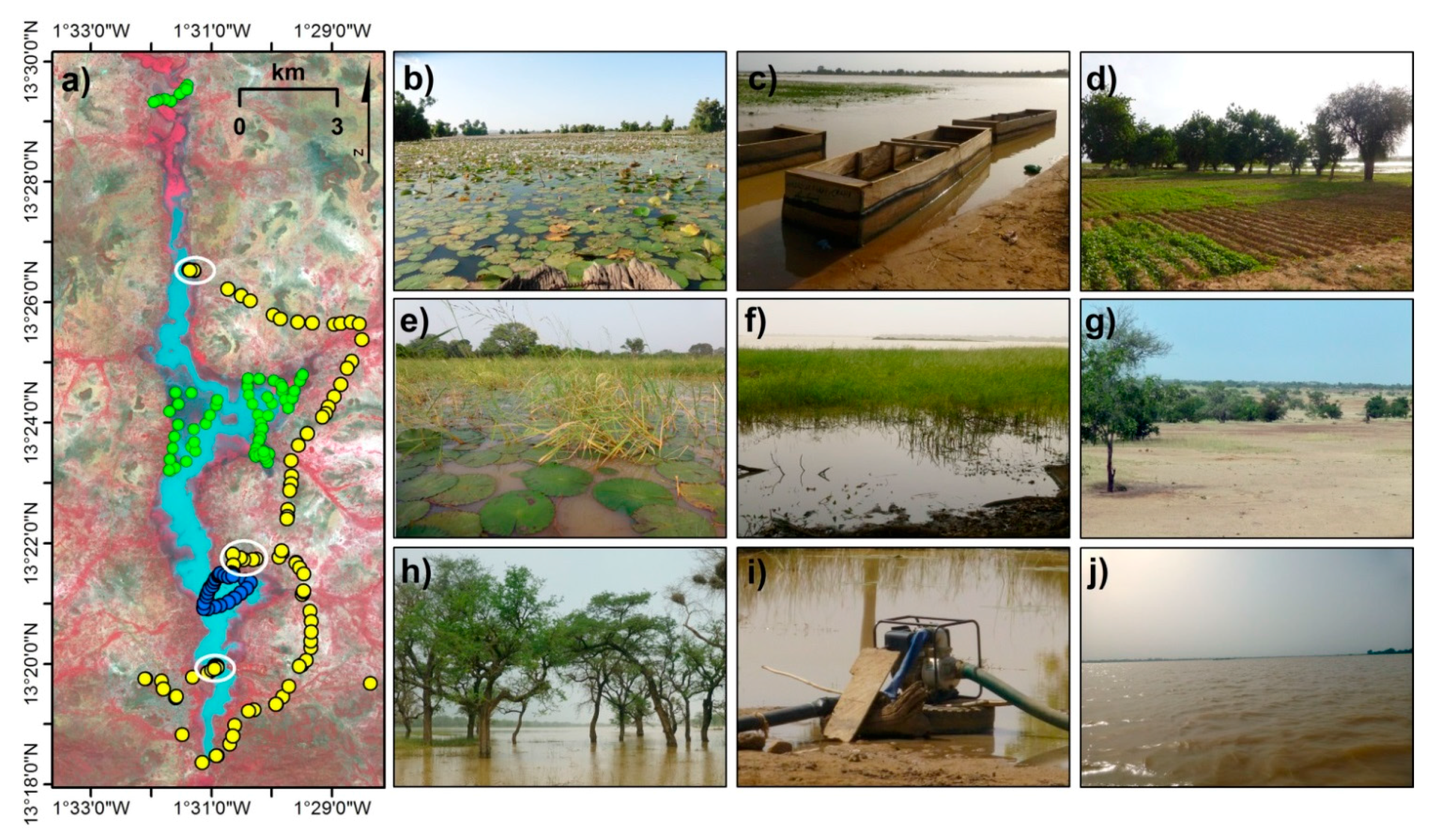
Remotesensing 08 00302 g001
Figure 2. (a) Location of the GPS data (from 15–18 October 2013 to 25–28 October 2015) with the (a) RapidEye image from 19 October 2013 as backdrop (©BlackBridge 2013, Berlin, Germany), including areas visited in greater detail (white circles), GPS/photo points on land (yellow dots), GPS/photo points from the boat tracks on the open water (blue dots), and on water with flooded vegetation (green dots); (b) floating water lilies; (c) shoreline including soil exposed after water retreat and flooded vegetation in the background; (d) irrigated fields; (e) flooded and floating vegetation; (f) water, flooded vegetation, and an island in the background, seen from the eastern shoreline; (g) barren land; (h) flooded trees next to the dam in the south; (i) motor pump at the shoreline; (j) open water seen from the boat southwards, (photos by L. Moser, F. Betorz Martìnez, R. Ouedraogo).
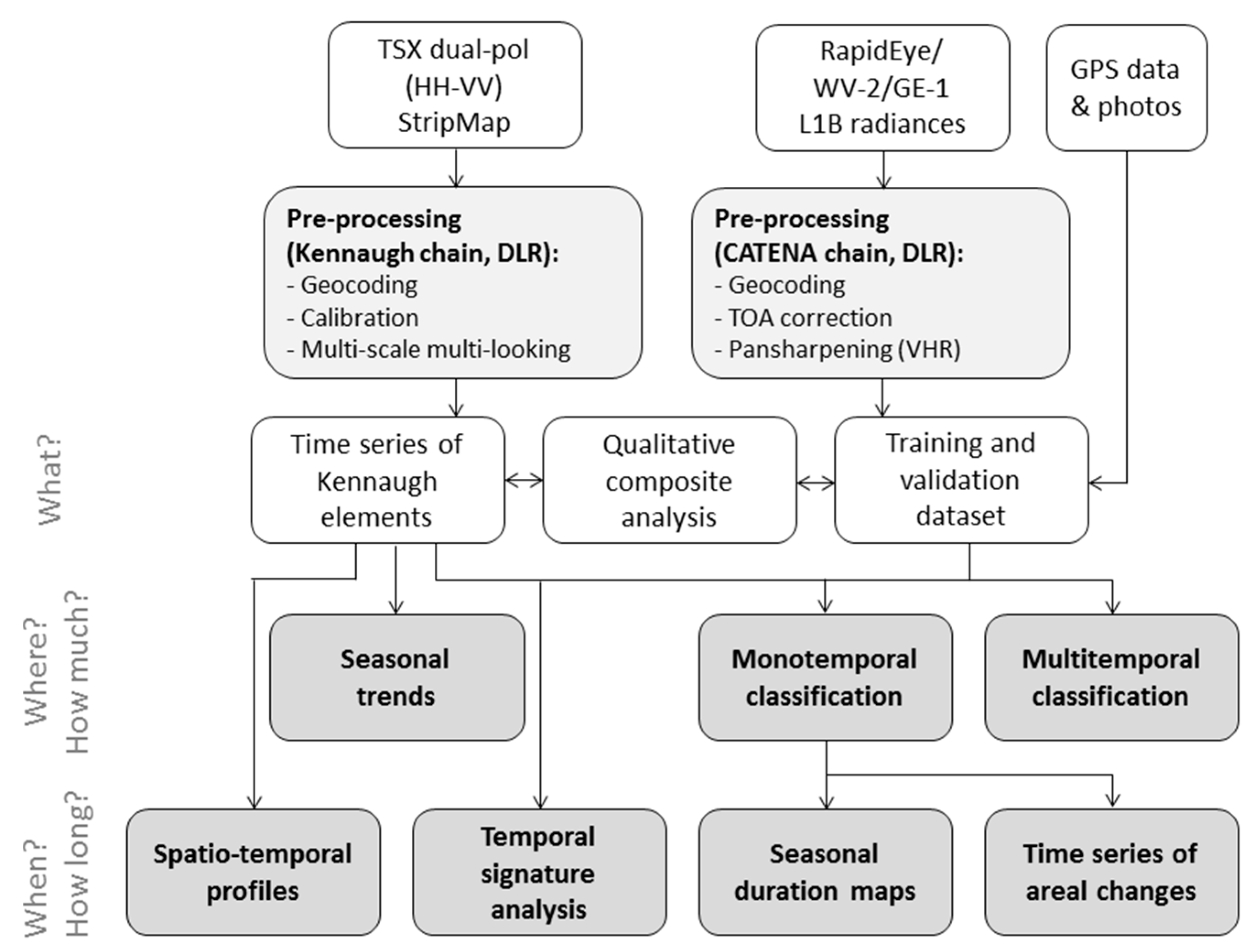
Remotesensing 08 00302 g002
Figure 3. Processing workflow.
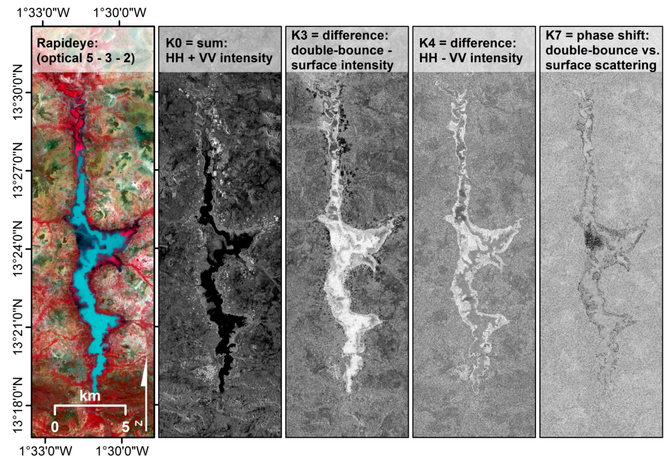
Remotesensing 08 00302 g003
Figure 4. From left to right: A RapidEye false color composite (band 5-3-2, i.e., NIR-red-green) reference image from 19 October 2013 (©BlackBridge 2013); the four Kennaugh elements derived from the dual-pol TSX image from 20 October 2013 (©DLR 2013): K0 (the total intensity as sum of HH plus VV intensity); K3 (difference double-bounce minus surface scattering); K4 (difference HH minus VV intensity); K7 (phase shift between double-bounce and surface scattering).
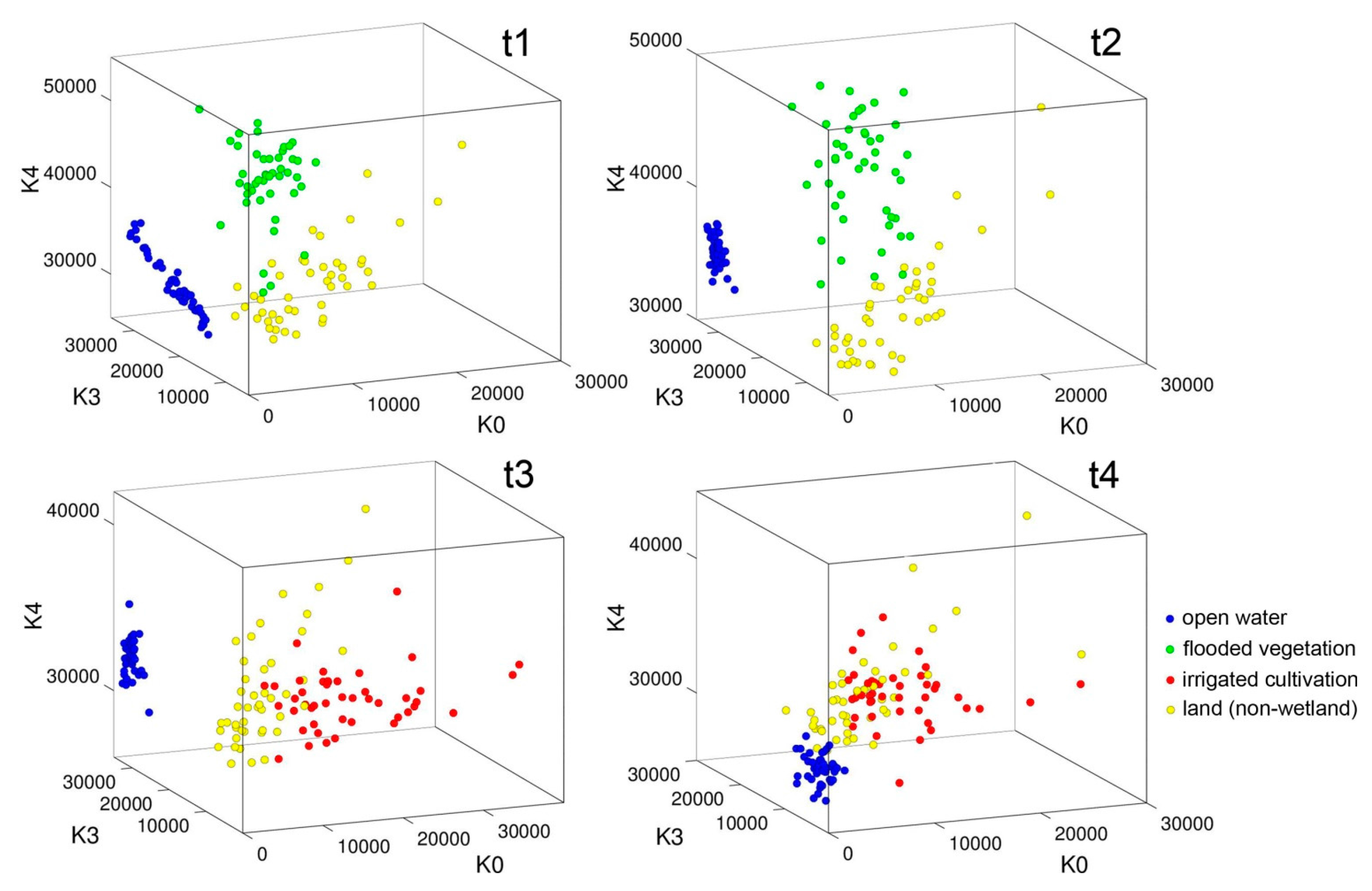
Remotesensing 08 00302 g004
Figure 5. Scatterplots for the Kennaugh elements K0, K3, and K4 displaying the mean value of each class of all 135 training and validation areas per time step: open water (blue), flooded vegetation (green), irrigated cultivation (red), and land (yellow), for four time steps (t1–t4). The Kennaugh elements are displayed in normalized scaling to 16 bit unsigned integer.
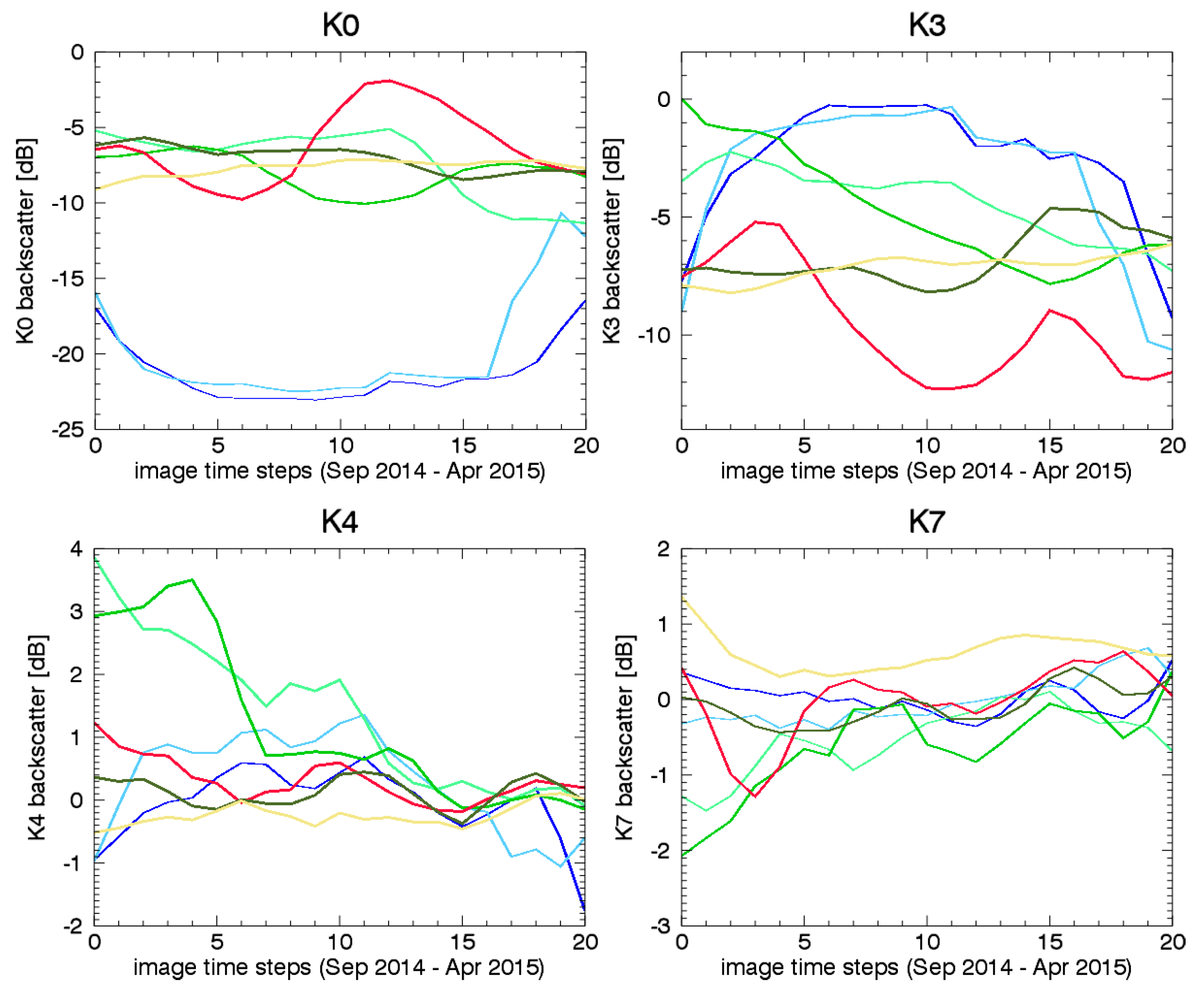
Remotesensing 08 00302 g005
Figure 6. Temporal signature analysis from September 2014 until April 2015 for the Kennaugh elements K0, K3, K4, and K7: W (dark blue); W–L (light blue); V–L (light green); V–F (green); L–F/F–L (dark red); L1 (dark green); L2 (beige).
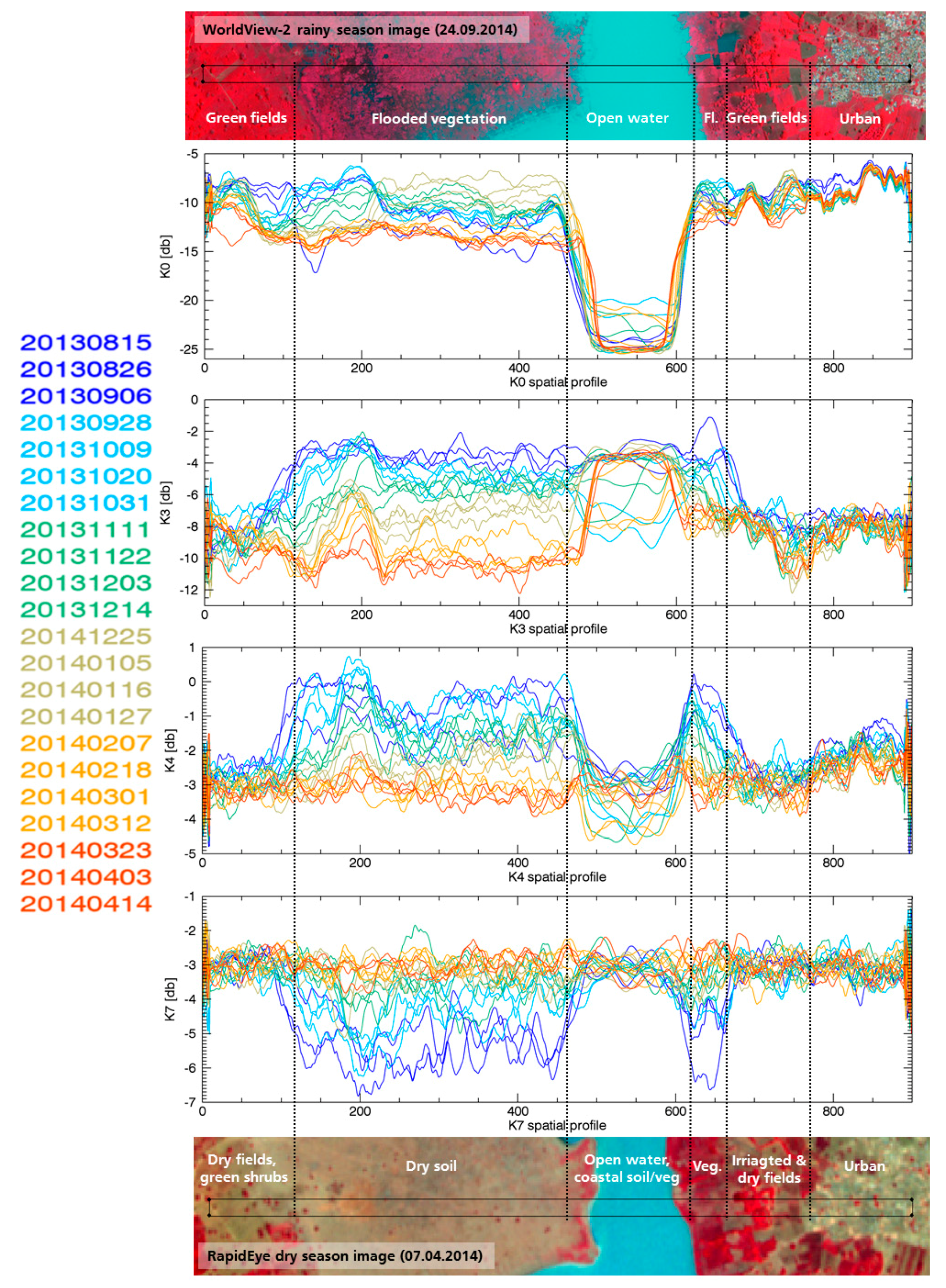
Remotesensing 08 00302 g006
Figure 7. Spatio-temporal profiles for different land cover types along the spatial profile with time steps of TSX Kennaugh elements visualized in the color scale. Optical reference images from WorldView-2 (24 September 2014) (©DigitalGlobe 2014 provided by EUSI, Westminster, CO, USA), and RapidEye (7 April 2015) (©BlackBridge 2014, Berlin, Germany) define the land cover during the start and end point of the temporal development.
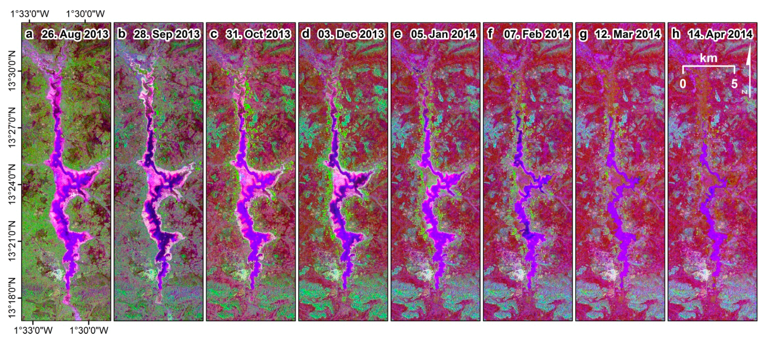
Remotesensing 08 00302 g007
Figure 8. Time series of eight selected HH-VV polarized TerraSAR-X (TSX) StripMap acquisitions from (a) 26 August 2013; (b) 28 September 2013; (c) 31 October 2013; (d) 3 December 2013; as well as (e) 5 January 2014; (f) 7 February 2014; (g) 12 March 2014; and (h) 14 April 2014 (©DLR 2013–2015). False color composites have been created from the Kennaugh elements (K4-K0-K3). Open water appears in blue/purple, green colors stand for vegetated or irrigated areas, and pink colors are dominant in areas of flooded vegetation.
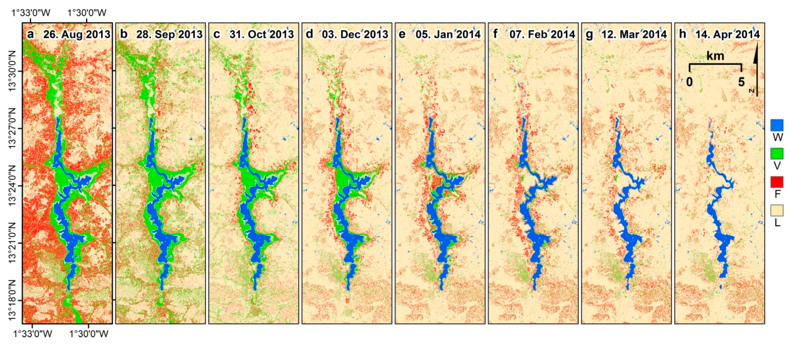
Remotesensing 08 00302 g008
Figure 9. Monotemporal classification for eight selected time steps with intervals of 33 days between the data: open water (blue); flooded/floating vegetation (green); irrigated fields (red); and dry land (beige) for (a) 26 August 2013; (b) 28 September 2013; (c) 31 October 2013; (d) 3 December 2013; as well as (e) 5 January 2014; (f) 7 February 2014; (g) 12 March 2014; and (h) 14 April 2014.
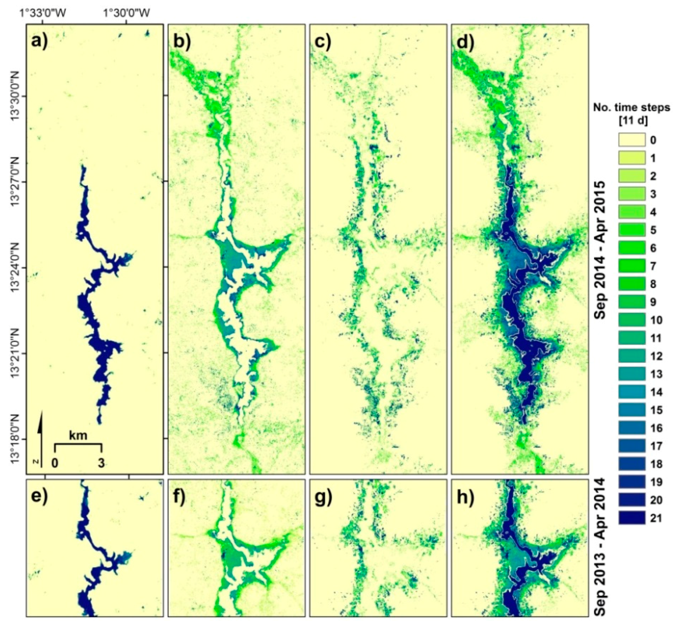
Remotesensing 08 00302 g009
Figure 10. Cumulative season duration areas of 21 time steps of the year 2014–2015 for (a) open water; (b) flooded/floating vegetation; (c) irrigated fields; and (d) wetland, and (eh) selected focus region for the year 2013–2014 below.
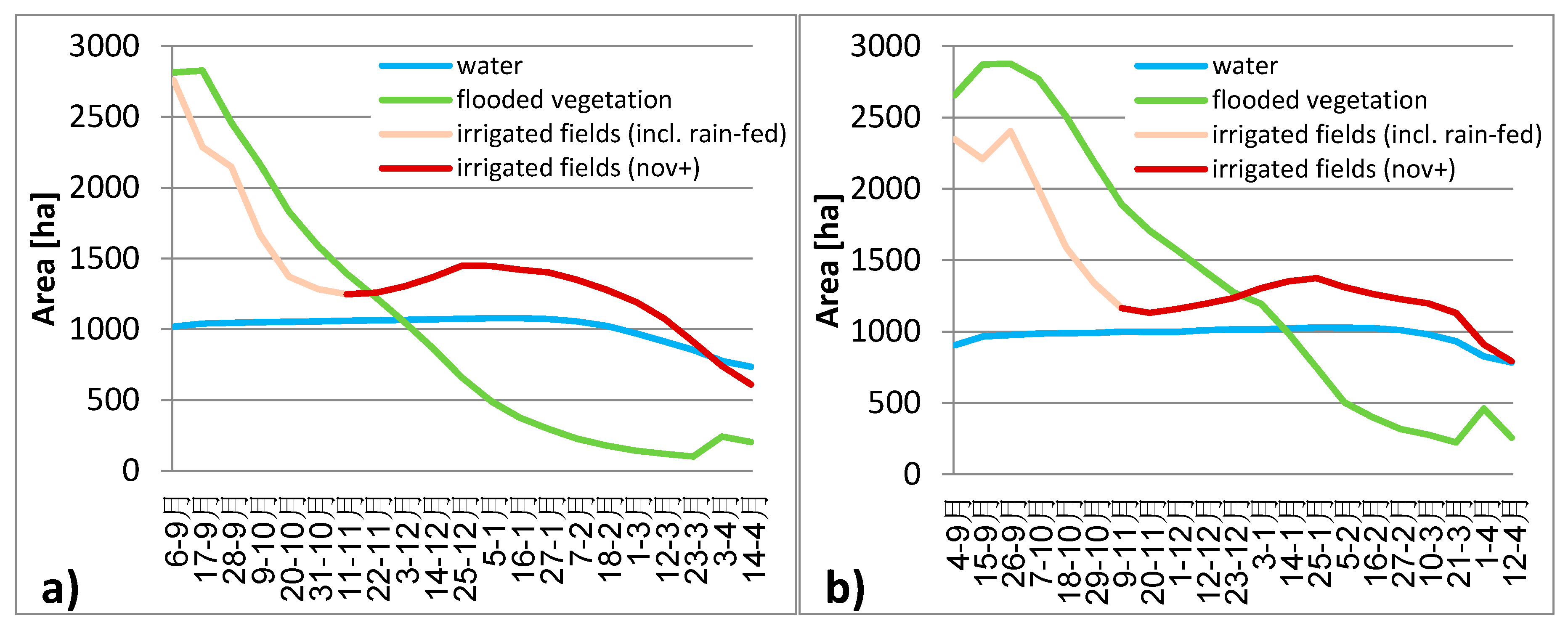
Remotesensing 08 00302 g010
Figure 11. Time series of the wetland area per class for (a) 2013–2014 and (b) 2014–2015: open water (blue), flooded/floating vegetation (green), irrigated fields (dark red), and rain-fed cultivation (light red).
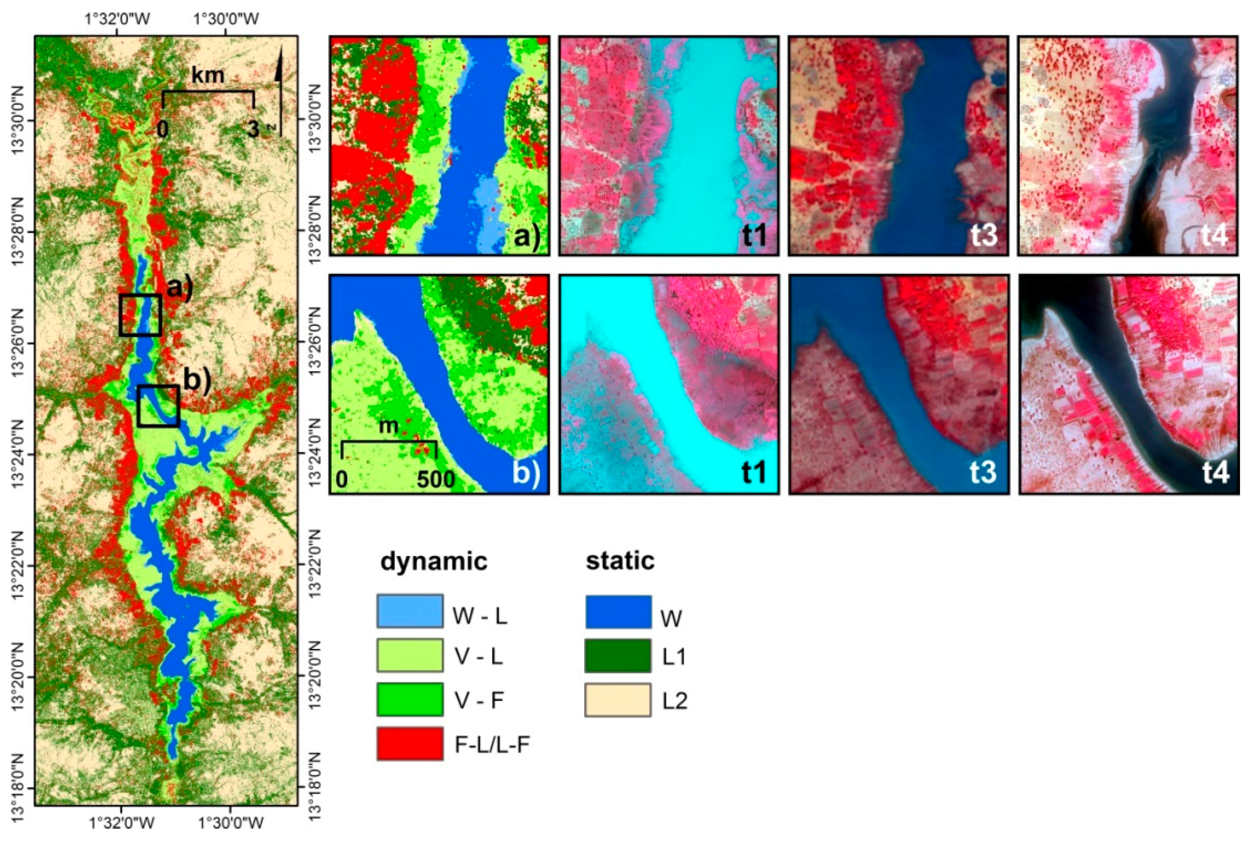
Remotesensing 08 00302 g011
Figure 12. Multitemporal classification for the time series stack of the year 2014–2015 resulting in seven change classes: open water (W); water to land/soil (W–L); flooded vegetation to land/soil (V–L); flooded vegetation to irrigated fields (V–F); and irrigated fields to land/soil or land/soil to irrigated fields (F–L/L–F); land with permanent vegetation (L1); and land with soil, rock, urban (L2). Two sites representing all classes are displayed in zoom windows: The northern site (a) features open water, the change from water to land, and large areas of cultivation in the east. The centrally located site (b) shows permanent open water, large areas that changed from flooded vegetation to land or to fields, and a permanently vegetated area in the north-east. Optical reference images (©DigitalGlobe 2014 provided by EUSI) for t1, t3, and t4 serve for comparison with the multitemporal classification results.
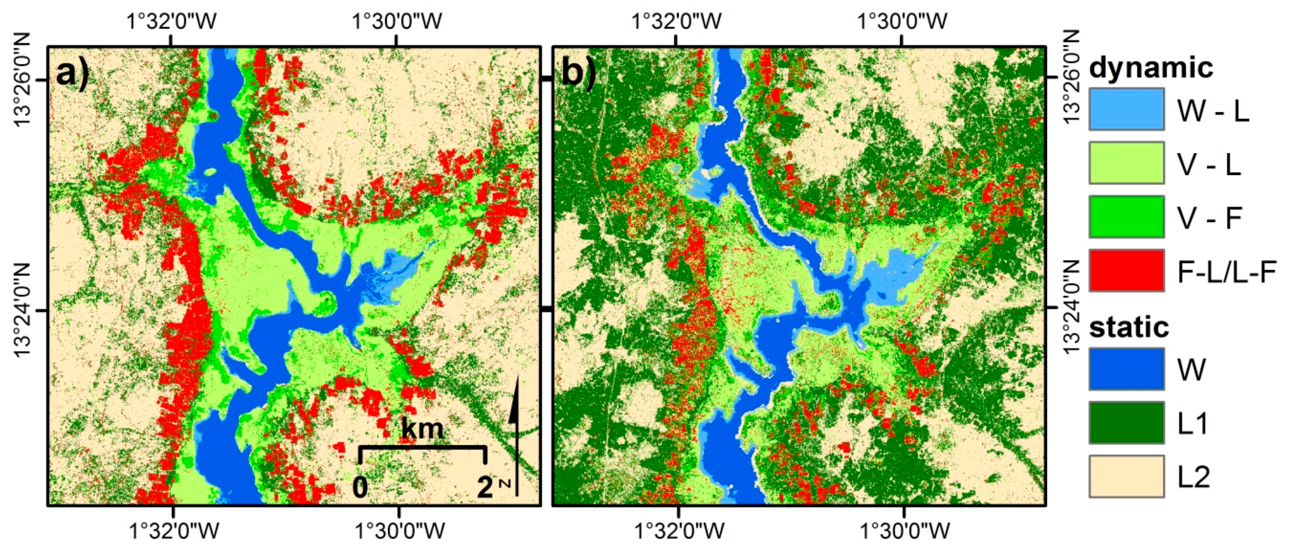
Remotesensing 08 00302 g012
Figure 13. Multitemporal classification results using as input (a) dual-polarimetric SAR intensity and phase data vs. (b) single-polarimetric SAR intensity (K0) only to classify the following change classes: open water—stable (dark blue); water to land (light blue); flooded vegetation to land (light green); flooded vegetation to field (green); irrigated fields (red); land with permanent vegetation—stable (dark green); and land with soil, rock, urban (beige).
Remotesensing 08 00302 g013
Table 1. Sensor characteristics of the used datasets TerraSAR-X, RapidEye, WorldView-2, and GeoEye-1.
TerraSAR-X RapidEyeWorldView-2GeoEye-1
Wavelength3.1 cmSpectral Bands440–510 nm (blue) 520–590 nm (green) 630–685 nm (red) 690–730 nm (redEdge) 760–850 (NIR)442–515 nm (blue) 506–586 nm (green) 624–694 nm (red) 765–901 (NIR)450–510 nm (blue) 510–580 nm (green) 655–690 nm (red) 780–920 (NIR)
ModeStripMap
PolarizationHH-VV dual-pol
FrequencyX-band (9.6 GHz)Dynamic range12 bits/pixel11 bits/pixel11 bits/pixel
Resolution6.60 m (azimuth), 2.49 m (range)Resolution6.5 m (ms)2 m (ms), 0.5 m (pan)2 m (ms), 0.5 m (pan)
Pixel spacing5 m (resampled)Pixel spacing5 m (resampled)0.5 m (pansharpened)0.5 m (pansharpened)
Inc. angle27.4°–28.9°Off-nadir angle2.5°–21.2° (different acquisitions)22.0°39.2°
Swath width15 kmSwath width77 km16.4 km15.2 km
Pass directionAscending, right-lookingPass directionDescendingDescendingDescending
Product levelLevel 1B (single Look Slant Range Complex (SSC))Product levelLevel 1B (basic)Level 1B (ortho-ready standard)Level 1B (ortho-ready standard)
Table 2. Remote sensing data used in this study. Main dataset: TerraSAR-X dual-co-polarimetric HH-VV StripMap time series. Reference datasets: RapidEye (RE), WorldView-2 (WV-2), GeoEye-1 (GE-1), and GPS/photo data. Data marked in bold were used as reference datasets for the areas of interest (AOIs).
2013–20142014–2015
NoTerraSAR-X DataOptical Reference DataGPS/Photo DataTerraSAR-X DataOptical Reference DataGPS/Photo Data
16 September 2013 4 September 2014
2* 17 September 2013 15 September 2014
328 September 2013 * 26 September 201424 September (WV-2)
49 October 2013 7 October 2014
520 October 201319 October (RE)15/18 October18 October 2014
631 October 2013 29 October 2014
711 November 2013 9 November 20148 November (RE)
822 November 2013 20 November 2014
93 December 2013 1 December 2014
1014 December 2013 12 December 2014
1125 December 2013 23 December 2014
125 January 2014 * 3 January 20155 January (RE)
1316 January 2014 14 January 2015
1427 January 2014 25 January 2015
157 February 20147 February (RE) 5 February 20152 February (RE)
1618 February 2014 16 February 2015
171 March 2014 27 February 2015
1812 March 2014 10 March 2015
1923 March 2014 21 March 2015
203 April 20147 April (RE) 1 April 201530 March (RE)
2114 April 2014 12 April 201515 April (GE-1)
25/28 October
* Three TSX datasets were temporally interpolated.
Table 3. Change processes at Lac Bam from the rainy to the dry season, illustrated for the four time steps: 24 September 2014 (t1), 8 November 2014 (t2), 2 February 2015 (t3), and 15 April 2015 (t4): W (water), V (flooded/floating vegetation), F (irrigated fields), L (dry land), main change processes are marked bold.
Change ClassStable/Dynamict1 (24 September 2014)t2 (8 November 2014)t3 (2 February 2015)t4 (15 April 2015)
WstableWWWW
W–LdynamicWWWL
WWLL
V–LdynamicVVVL
VVLL
V–FdynamicVVLF
F–L/L–FdynamicFLFL
LFFL
LLFL
LLLF
L1stableLLLL
L2stableLLLL
Table 4. Areas of interest (AOIs) for the training dataset (averaged for t1–t4) and validation dataset (for each image t1–t4) of the monotemporal classification applied on each image in the time series: W (water); V (flooded/floating vegetation); F (irrigated fields); L (land).
WVFLSum AOIs per Time Step
Training t125 (av. t1–t4)25 (av. t1–t2) 25 (av. t1–t4)100 (t1–t4)
Training t225 (av. t1–t4)25 (av. t1–t2) 25 (av. t1–t4)
Training t325 (av. t1–t4) 25 (t3 only)25 (av. t1–t4)
Training t425 (av. t1–t4) 25 (av. t1–t4)
Validate t120 (t1–t4)20 (t1–t2) 20 (t1–t4)60 (t1)
Validate t220 (t1–t4)20 (t1–t2) 20 (t1–t4)60 (t2)
Validate t320 (t1–t4) 20 (t3 only)20 (t1–t4)60 (t3)
Validate t420 (t1–t4) 20 (t4 only)20 (t1–4)60 (t4)
Sum AOIs per class45 (t1–t4)45 (t1–t2)65 (val. t3 differs t4)45 (t1–t4)
Table 5. Multitemporal AOIs for the training and validation dataset: W (water); W–L (water to land/soil); V–L (flooded vegetation to land/soil); V–F (flooded vegetation to irrigated fields); F–L/L–F (irrigated fields to land/soil or land/soil to irrigated fields); L1 (land: permanent vegetation); L2 (land: soil, rock, urban).
W StableW–L DynamicV–L DynamicV–F DynamicF–L/L–F DynamicL1 StableL2 StableSum AOIs Multitemp
Training Multitemp2525252525817150
Validate Multitemp2020202020713120
Sum AOIs per Class45454545451530
Table 6. Accuracy assessment of the monotemporal classification t1 (24 September 2014), t2 (8 November 2014), t3 (2 February 2015), t4 (15 April 2015), with Producer’s Accuracy (PA) and User’s Accuracy (UA) for each class, Overall Accuracy (OA) for each image, non-existing classes are marked as N/A.
T1 (24 September 2014)T2 (8 November 2014)T3 (2 February 2015)T4 (15 April 2015)
PA (%)UA (%)PA (%)UA (%)PA (%)UA (%)PA (%)UA (%)
Open Water99.999.1100.099.399.999.295.190.0
Flooded Veg.94.983.691.284.2N/AN/AN/AN/A
Irrigated fieldsN/AN/AN/AN/A82.168.669.266.1
Land56.293.461.791.660.485.463.274.1
OA (%)85.586.383.879.7
Table 7. Accuracy assessment of the multitemporal classification with the classes open water (W); water to land/soil (W–L); flooded vegetation to land/soil (V–L); flooded vegetation to irrigated fields (V–F); and irrigated fields to land/soil or land/soil to irrigated fields (F–L/L–F); land with permanent vegetation (L1); land soil, rock, urban (L2). The error matrix including Producer’s Accuracy (PA) and User’s Accuracy (UA) are stated for each class.
W (st.)W–L (dyn.)V–L (dyn.)V–F (dyn.)F (dyn.)L1 (st.)L2 (st.)PA (%)UA (%)
Water(stable)440753500000100.089.2
Water to Land(dynamic)09960000058.8100.0
Flooded Veg. to Land(dynamic)0129219610673890.189.7
Flooded Veg. to Field(dynamic)02222110239208584.975.0
Land (Perm. Veg.)(stable)0081410924115686.483.3
Irrigated Fields(dynamic)0291607920104696.890.3
Land (Soil, Urban)(stable)041016472134682.094.5
Table 8. Accuracy assessment of the multitemporal classification using a stack of all time steps of all four Kennaugh elements (left), compared to using only K0 (right).
K0-K3-K4-K7K0
PA (%)UA (%)PA (%)UA (%)
water (stable)100.088.598.7100.0
water to land (dyn.)56.6100.098.198.7
flooded veg. to land (dyn.)90.189.779.087.0
flooded veg. to field (dyn.)84.975.044.742.1
land/perm. veg. (stable)86.483.357.649.5
irrigated fields (dyn.)96.890.379.083.7
land/soil/urban (stable)82.094.578.973.7
OA (%)88.582.2

