Automatic Geometric Processing for Very High Resolution Optical Satellite Data Based on Vector Roads and Orthophotos

Abstract

In response to the increasing need for fast satellite image processing SPACE-SI developed STORM—a fully automatic image processing chain that performs all processing steps from the input optical images to web-delivered map-ready products for various sensors. This paper focuses on the automatic geometric corrections module and its adaptation to very high resolution (VHR) multispectral images. In the automatic ground control points (GCPs) extraction sub-module a two-step algorithm that utilizes vector roads as a reference layer and delivers GCPs for high resolution RapidEye images with near pixel accuracy was initially implemented. Super-fine positioning of individual GCPs onto an aerial orthophoto was introduced for VHR images. The enhanced algorithm is capable of achieving accuracy of approximately 1.5 pixels on WorldView-2 data. In the case of RapidEye images the accuracies of the physical sensor model reach sub-pixel values at independent check points. When compared to the reference national aerial orthophoto the accuracies of WorldView-2 orthoimages automatically produced with the rational function model reach near-pixel values. On a heterogeneous set of 41 RapidEye images the rate of automatic processing reached 97.6%. Image processing times remained under one hour for standard-size images of both sensor types.

1. Introduction

The ever increasing quantity of satellite data from large and small Earth observation satellites offers the potential for new and innovative applications and boosts the need for automatic and fast data processing. However, complex and slow data processing remains the main obstacle that prevents most end users from using satellite data. Although the image processing steps are usually known, they are neither automatic nor performed in real-time. Fully automatic and generic (i.e., adapted to different sensors) systems for processing high resolution (HR; from 10 m to 2 m) and very high resolution (VHR; 2 m and below) optical images are predominantly demanded by the Earth observation community.

All optical image processing—either automatic or manual—includes several pre-processing and product generation steps. The obligatory pre-processing steps are composed of geometric and radiometric corrections in which the pixels’ locations and values are corrected. The product generation stage is optional, application oriented and generates thematic products that are aimed at end-users. Although this common two-stage roadmap is well-defined, the details of individual processing workflows vary substantially, for they depend on the sensor type, processing level of the input image and the user’s needs (e.g., if an orthoimage represents the final goal, only geometric corrections are applied). In this paper we will focus on the automatic geometric corrections of the STORM processing chain developed by the Slovenian Centre of Excellence for Space Sciences and Technologies (SPACE-SI). (The STORM processing chain developed by SPACE-SI is not to be confused with Apache’s system for generic real-time computation known as Apache Storm (http://storm.apache.org/). The two systems are not connected in any way.)

Automated processing steps are the best way of tackling large volumes of satellite images. A variety of automatic or semi-automatic processing systems is used by various optical satellite data vendors or providers, as well as by many application-oriented companies specializing in Earth observation. However, these systems are proprietary, in most cases sensor-specific and confidential, thus they are usually not described in scientific papers. As a result, merely a handful of papers have been published on this topic. The rare examples include e.g., CATENA, developed at the German Aerospace Center (DLR), Remote Sensing Software Package Graz, developed at Joanneum Research, and the GeoCDX system developed at the University of Missouri, Columbia. CATENA, developed in 2006 (e.g., [1]), is a highly advanced generic modular operational infrastructure for automatically processing optical satellite and airborne image data. It uses an area-based image that is matched to an orthorectified reference image [2] with which it extracts ground control points (GCPs). Several thousand images have already been processed with this chain, e.g., Fast Track Land Services Image2006, –2009 and –2012 for ESA GMES. A similar modular system can be found in the Remote Sensing Software Package Graz developed by Joanneum Research—the beginnings of which reach back into the 1980s [3]—which is also able to process synthetic aperture radar images. GeoCDX, a resolution-independent system for fully automated change detection on HR and VHR satellite imagery [4], is designed to process and exploit large volumes of images. The geometric corrections are based on image co-registration. The ultimate aim of this system is to change the detection between previously co-registered and radiometrically standardized image pairs.

Several studies on the automation of geometric corrections have been performed over the past decades. Bignalet–Cazalet et al. [5] automated the mosaicking of Pleiades level 1A images (with a nadir spatial resolution of 70 cm for the panchromatic band) by placing each included image into a shared geometry, homogenizing their radiometry, and finally generating an orthomosaic with the use of stitching lines. Eugenio and Marqués [6] automated the georeferencing of low and middle resolution images by extracting the GCPs with the use of the contour-matching approach. Gianinetto and Scaioni [7] developed the Automatic Ground control points Extraction technique (AGE). In order to obtain the coordinates of the reference points an adaptive least squares matching is performed between the raw and the georeferenced image. The algorithm was successfully tested on Quickbird, SPOT 5 and IKONOS images. Leprince et al. [8] developed an almost completely automatic orthorectification of optical satellite images for the use in ground deformation measurements. The correlation between the images is performed via the phase correlation method, which relies on the Fourier shift theorem. This means that the relative displacement between a pair of similar images is obtained from the phase difference of their Fourier transform. Prior to the orthorectification one needs to manually locate the GCPs on all images. This process has been developed for SPOT 5 images. Liu and Chen [9] created an effective process for automatic orthorectification of high resolution Formosat-2 images. Their method correlates ground control regions from orthophotos and satellite images. Orthorectification uses a physical model and achieves accuracy below 1.5 pixels. Devaraj and Shah [10] also developed an automatic geometric correction process. The orthorectification of medium-resolution CBERS-2 and CBERS-2B images is performed with reference to Landsat imagery. Prior to undertaking the correlation step the previously orthorectified Landsat images are transformed into their raw form (geometric distortions are introduced) after which the registration is performed by affine transformation.

Several automatic geometric correction procedures have been successfully attempted with the rational function model (RFM). For example, Oh and Lee [11] developed an algorithm for automatic bias-compensation of rational polynomial coefficients (RPCs) based on topographic maps. Their matching accuracy was approximately one pixel.

Studies addressing the automatic registration of satellite images onto the reference vector layer date back to 1998 ([12]). Several types of imaging features such as lines and polygons, and different types of vector data (road network, forest areas, houses etc.) were selected for registration, e.g., Hild and Fritsch [12] presented a system which utilises forest area polygons matched to the vector data of land use. Numerous studies used road or line segments (e.g., [13,14,15,16]), however these studies were not realised in actual applications. Kruger [17] presented an efficient framework in which the extraction of line segments and matching were not separated, for they were formulated as a projective transformation parameter estimation problem which can be efficiently solved. However, this type of image-to-map registration has not yet been proven as a working and reliable satellite image processing system.

This paper presents a completely automated procedure for precise orthorectification of optical satellite images that is used within the STORM processing chain. In order to extract the GCPs two- and three-step algorithms (depending on the resolution of the input images, starting with image to rasterized roads and finishing with super-fine image to aerial orthophoto matching) were implemented. Our proprietary physical sensor model and RFM were implemented for the geometric modelling. At the end the images were indirectly orthorectified with the use of a digital elevation model (DEM). The proposed procedure is generic and can fit various HR and VHR satellite images.

If one wishes to produce a final output with a desired accuracy without the need for the operator’s intervention, validation or correction, the algorithms need to be highly reliable and robust with respect to the varying imaging conditions. However, the quality of input images varies due to seasonal variations, daily atmospheric conditions and the imaging geometry. The most challenging image quality factors include snow, clouds and haze, low contrast of ground features as a result of low illumination or the presence of cloud shadows, image deformations occurring due to the off-nadir viewpoint and terrain elevation, and temporal variations of the vegetation and man-made objects. Due to their long-term stability and high visibility, roads were selected as a suitable reference feature to help us cope with these problems. The automatic GCP extraction algorithm presented in Section 3.1 and Section 3.2 was designed to address the image quality problems with the use of several criteria for detecting the most suitable GCPs and by providing estimated measures for their quality. This enables the sensor model and the orthorectification algorithm (Section 3.3 and Section 3.4) to perform robust iterative optimization and remove outlying GCPs and thus come up with accurate registration.

The following requirements were set before the STORM processing chain was developed:

-

Robustness: automatically process at least 90% of all images

-

Speed: processing time for a standard size image should be under one hour

-

Accuracy of the extracted GCPs and the final orthoimages: root-mean-square-error (RMSE) bellow one pixel (i.e., 6.5 m) for HR RapidEye images and bellow two pixels (i.e., 4 m) for VHR WorldView-2 multispectral images. Based on the experience gained from the existing processing practices, the thresholds for VHR images were set differently from those for HR images as different resolutions result in different processing challenges.

A diverse and comprehensive data set of 41 HR RapidEye images and nine VHR WorldView-2 images (Section 4 and Section 5) were used to show and evaluate to what extent the initial requirements were met.

The STORM processing chain is composed of numerous steps that are combined into an extremely robust automatic system with a unique implementation. Great efforts were made to push the technology in the direction of full automation. The suggested process is especially innovative in the GCPs extraction based on reference road layers and geometric modelling with incorporated gross error removal steps. The manuscript presents the most relevant parts of the implemented geometric corrections which are extremely complex and contain numerous iterative steps that guarantee the stability and validity of the results. Even though these iterations and controls are important for the operation of the chain, they are not helpful to the reader and are thus not explicitly presented in the manuscript.

The overall concept and workflow of the STORM processing chain is described in the following section. Section 3 deals with the algorithms used in individual sub-modules of the geometric corrections module. Section 4 describes the used data and the accuracy evaluation measures. Section 5 delivers the results of the sub-modules of the geometric corrections on an extended set of HR RapidEye images and VHR WorldView-2 images. The outcomes are discussed in Section 6, while the summary of the results can be found in the Conclusions.

2. The STORM Automatic Processing Chain

In the search for a generic and fast processing system, SPACE-SI (the Research Centre of the Slovenian Academy of Sciences and Arts has contributed to the development of individual algorithms.) has developed and implemented STORM—a fully automatic image processing chain that performs all processing steps from sensor-corrected (usually denoted as level 1; pixel values are at-sensor radiances) or ortho-ready (level 2) optical satellite images to web-delivered map-ready products. The processing chain is generic, modular, works without the operator’s intervention, and fully supports RapidEye images of Slovenia and its surroundings. Various parts of the chain were implemented also for WorldView-2, THEOS, Pleiades, SPOT 6, Landsat 5–8, and PROBA-V images.

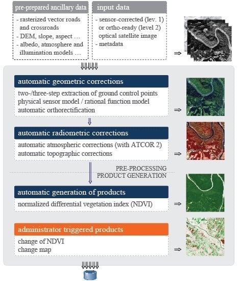
The STORM processing chain (Figure 1) follows the commonly accepted two-stage processing workflow for optical imagery, beginning with pre-processing and ending with the generation of the final product. The first step of the pre-processing stage focuses on geometric corrections. These are performed in two sub-modules: automatic extraction of GCPs based on matching them onto either reference rasterized roads (two-step algorithm) or reference rasterized roads and orthophotos (three-step algorithm), which is followed by automatic sensor modelling with orthorectification, during which either the proprietary physical sensor model or RFM are utilised. The details on the geometric corrections sub-modules are described in Section 3.

The second pre-processing step focuses on radiometric corrections performed through two sub-modules: firstly the atmospheric corrections are applied, and this is followed by topographic normalization. The state-of-the-art commercially available ATCOR 2 software package is used [18] to eliminate the effects of the atmosphere such as scattering and haze, and to define the extent of clouds and cloud shades. ATCOR 2 was fully integrated into the STORM workflow. In the process it is called directly from within the STORM's code. On the other hand, our proprietary algorithm [19] is used for topographic normalization. This combines the physical approach to topographic corrections with the Minnaert method [20], and utilizes the anisotropic illumination model [21] for various illumination situations and the Otsu algorithm [22] for the detection of shaded areas.

Once the pre-processing is completed, end-user products are generated. The STORM processing chain implements the automatic generation of normalized differential vegetation index (NDVI). Additionally, the administrator can manually trigger the computation of the change of the NDVI product, which compares two sequentially overlapping NDVI products, and changes the map product (e.g., [23]) with hot-spots depicting the changes between the two sequential images.

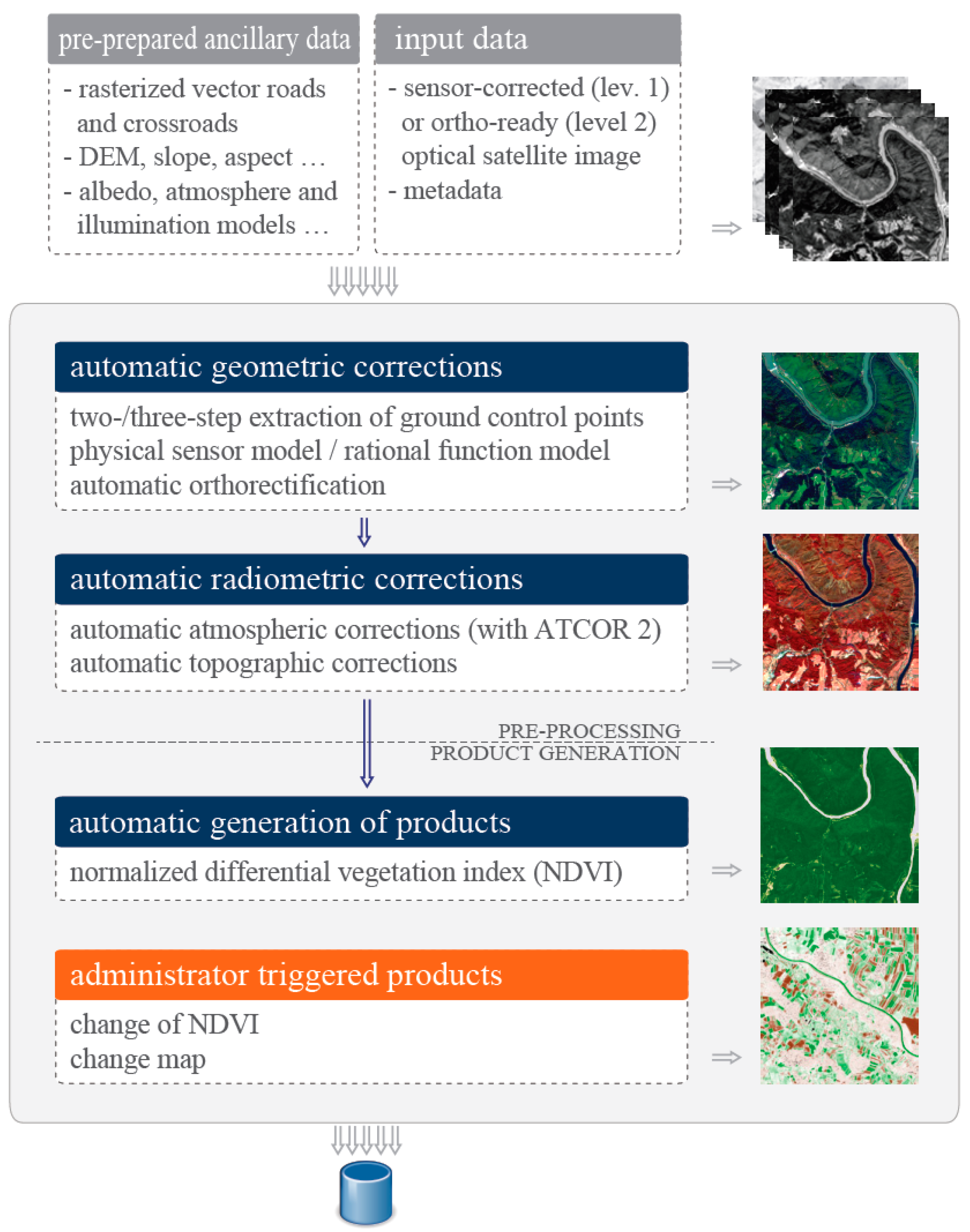
All output products (i.e., orthoimage, radiometrically corrected image, NDVI, change of NDVI, change map) that emerge from a single input image are stored in the database, together with the essential metadata on the processing strategy and parameters (Figure 1). At the end of the STORM processing chain, several interrelated services deliver data to end-users via the Java-developed web application, which enables basic web mapping operations, various attribute queries, spatial queries as well as downloading products including all processing information and metadata. The web application includes an administrative part for controlling the processes in the STORM processing chain.

Individual processing steps are prepared as independent IDL or C++ sub-modules which are controlled from the Java-based main control module (MCM). MCM ingests the input satellite data and prepares a new Java thread, in which the module execution commands of fixed order are prepared. The Java/IDL bridge is used to pass XML-encoded commands and parameters from MCM via the image processing server, which is basically a wrapper that runs the individual processing modules. MCM controls the processing resources as well as the execution of individual processing modules via log messages. On the processing side the XML-encoded files are interpreted, individual modules are executed, and upon completion the processing metadata is returned. On the other hand, the input and output images are stored in a file-based system on an image server, where they are accessed directly, while the XML files merely include the paths to their locations. MCM post-processing consists of writing output parameters to the PostGIS spatial object-relational database (Figure 2) and of image tiling. MCM is also used to communicate with web applications.

The main data entity for the database is represented by the input satellite image. The entity can have an arbitrary number of phases, which correspond to the processing modules. Each phase has a completion status flag and several input and output parameters. The database records the metadata from the input satellite image as well as the metadata from all processing phases and parameters.

3. Automatic Geometric Corrections

The STORM automatic geometric corrections module generates orthorectified satellite images by correcting the geometric distortions that appear on the input image due to relief and imaging geometry. Since the quality of all processing chain products depends on the quality and accuracy of the orthorectified satellite image this module is of utmost importance. High quality demands are made on the geometric corrections module as a whole as well as on all of its interdependent individual sub-modules; e.g., the accuracy of the extracted GCPs has a strong influence on the accuracy of the final orthoimage.

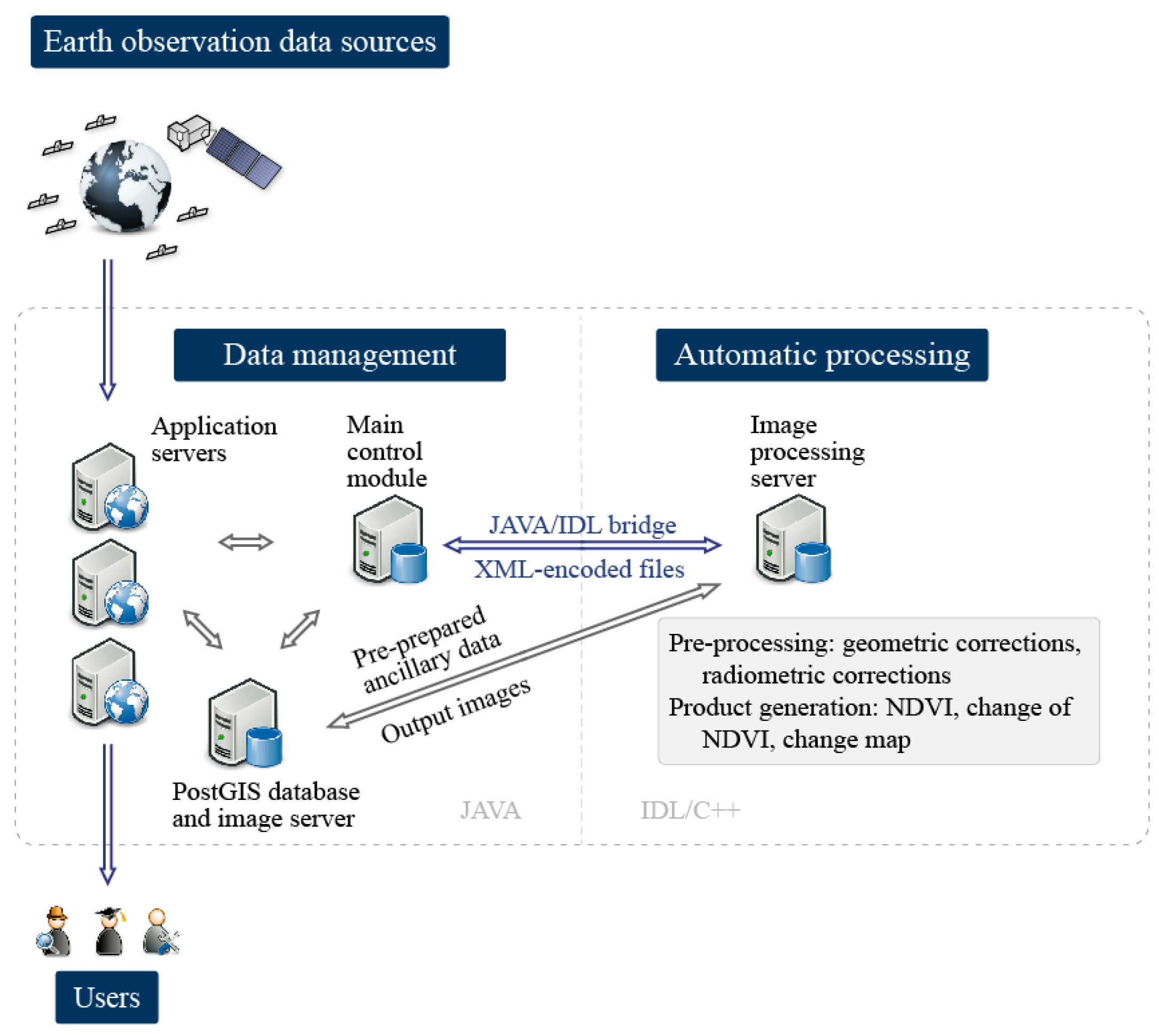
In the proposed workflow (Figure 3) the first GCPs are automatically extracted with the two-step image matching onto the reference rasterized roads (Section 3.1), while the three-step algorithm also uses aerial orthophotos as a reference layer for the additional super-fine positioning step (Section 3.2). The two-step algorithm is used for HR images, while the three-step algorithm is used for VHR images. The extracted GCPs are used as input data for the automatic orthorectification procedure which is based either on the physical sensor model (Section 3.3) or on the RFM (Section 3.4).

The listed algorithms were developed in a different order. During the initial development the goal was to automatically orthorectify the sensor-corrected level 1B RapidEye image—with a 6.5 m resolution—with the use of the two-step GCP extraction algorithm and the physical sensor model. In the following stages of development—when support for VHR sensors was added—we introduced substantial improvements to the GCP extraction. Furthermore, RFM was also introduced, and this served as an alternative for the physical sensor model and enabled the orthorectification of input images equipped with RPCs at higher processing levels (e.g., level 2 ortho-ready images, in which certain geometric corrections were already applied).

Some algorithms and results of the geometric corrections of the HR RapidEye system were partly presented in [24], therefore this paper focuses on the adaptation for the VHR WorldView-2 system.

3.1. Automatic Two-Step GCP Extraction Algorithm for HR Systems

Due to the temporal variability of the Earth’s surface, the varying atmospheric conditions (e.g., [25]) and geometric distortions the automatic extraction of GCPs from multi-temporal and multi-sensor images is a difficult task.

GCP extraction methods differ in terms of reference data to which the unregistered input image is compared, in terms of the features extracted from the image, as well as in terms of the underlying geometric transformation model. The area-based methods (e.g., [26]) that apply image-to-image coregistration are computationally expensive and may be unreliable due to false matches. The feature-based methods start by extracting distinct low-level image features such as corners or other distinct points (e.g., [27]) from both, the unregistered and reference image, and then they estimate the geometric transformation among the pairs of points. The image-to-map registration methods use higher-level image primitives such as lines (e.g., [15]) or polygons (e.g., [12]) extracted from the unregistered image and compare them to a vector objects database such as a road network.

We tested the feature-based and area-based algorithms with the use of national aerial orthophotos as reference images, however we could not obtain satisfactory results. This was mainly due to the difference in the quality and dates of acquisition, for the unregistered and reference images were created several years apart and at different spatial resolution. In the end we adopted the image-to-map approach, as the road layers proved to represent a stable reference source, thus providing the required reliability of the extracted GCPs. Furthermore, the road network proved to be a structure that can be reliably detected on rural and semi-urban HR satellite images with rather straightforward image processing such as colour segmentation and line detection (e.g., [28,29,30,31]). Additional advantages of using roads can be found in the fact that they are easily visually recognised, that they lie on the Earth’s surface (ground), and that they are (especially crossroads) commonly used in the manual GCP selection process. Using roads as a reference source makes the automatic procedure similar to the manual procedure.

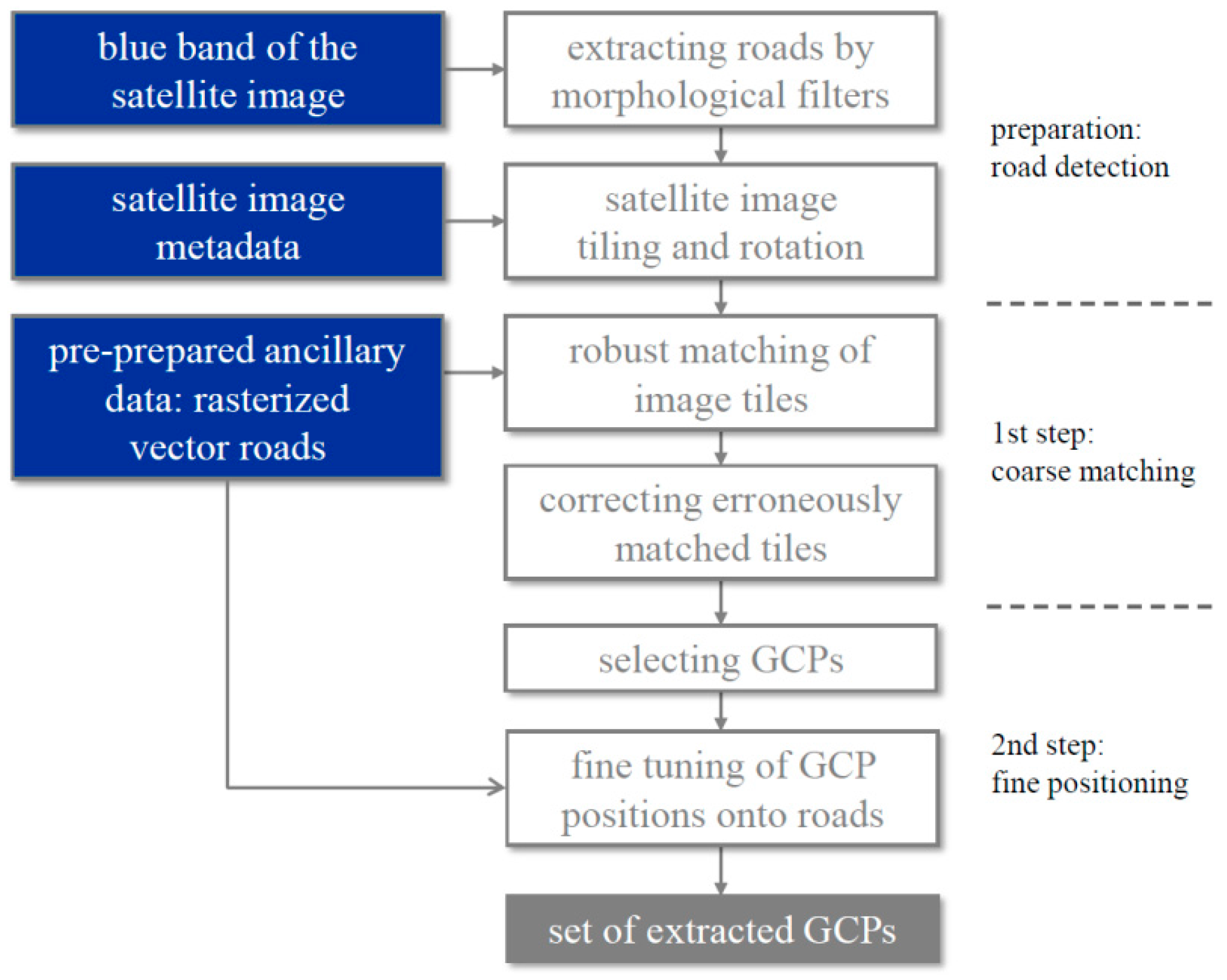
The proposed automatic GCP extraction algorithm [32] matches the roads detected on the satellite image to the reference rasterized vector roads (Figure 4). This is different from the majority of other methods, which optimise the transformation parameters within a vector space (e.g., [17]). Our method enables the preparation of the reference rasterized roads in advance. Rather than using a single global mapping function for the entire satellite image, the image is divided into tiles, which are later on matched individually. In the end the positions of potential GCPs are locally refined.

However, in order for this method to work, one needs an accurate reference road layer throughout the image. For the area of Slovenia we have used two different national vector road databases. Our primary source was the topographic vector road data at a scale 1:5.000 with 1 m planar accuracy and high road density (including e.g., also trails and cart tracks), however this only covers 60% of Slovenia and was last updated in 2008. This was complemented with the vector road data of the national public infrastructure cadastre (dated November 2012), with a planar accuracy under 1 m and 1–5 m for highways and other roads. This source has a lower road density than the primary one, however it is updated regularly. For the neighbouring countries we used the OpenStreetMap vector road data (retrieved on 3 March 2013). This data is updated by volunteers, therefore it is incomplete and lacks accuracy information. All vector data was rasterized based on the road width attribute (topographic roads) or road category attribute (public infrastructure roads, OpenStreetMap roads). As a rule, only roads wider than 3 m were used in our procedure.

Since they exhibit higher reflectance than the surrounding areas roads appear as bright lines on all visible bands of the satellite image. The proposed road detection algorithm was applied to the blue band of the image, as this band provided the best contrast between the roads and the background. Road detection is based on the morphological image filtering that uses top-hat transformation of a predefined size (e.g., [33]), which detects bright road candidate segments. The result is a binary mask of road candidates. The used method applies an adaptive histogram stretch, which increases the contrast of the road pixels against the background and is also able to tackle more challenging conditions with complicated atmospheric situations (haze, clouds, cloud shades).

We were also able to process winter images with snow-covered areas, where the intensities are inversed (dark roads on bright snowy surroundings). Since we did not perform any prior snow detection this adaptation was automatically applied to all bright regions on the input band with values above the upper value used in the histogram stretch. Firstly, the bright regions were dilated so that they included roads and other adjacent features. Their histograms were stretched so that all bright pixel values were flattened into a single value, and finally the resulting values were inverted. This enabled the same top-hat operator to be applied to the entire image.

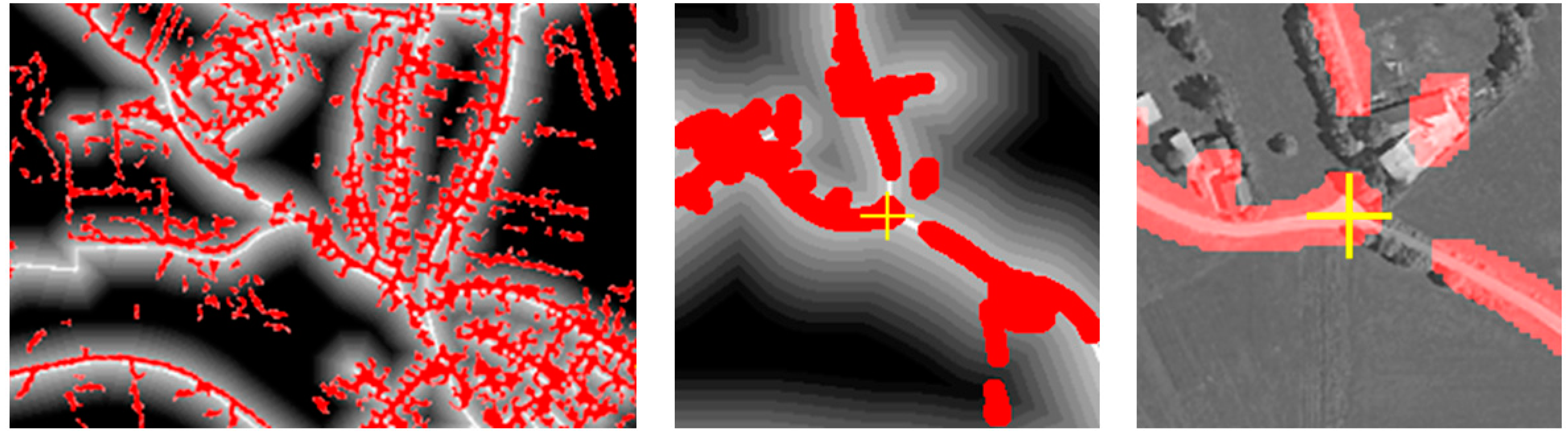
Firstly, the obtained binary mask of the road candidates is rotated by an angle calculated from the satellite image metadata and tiled based on the image size. A standard-sized RapidEye image is tiled into 8 × 8 tiles, at which the typical tile-size measures 1500 × 950 pixels. Tiling allows for an efficient parallelization of the GCP extraction process. The first step of the matching process performs robust estimation of nine perspective transformation parameters by minimizing the correlation-based distance between satellite road tiles and the road distance image (i.e., distance from the centre of the road) (Figure 5, left). The algorithm requirements for coarse matching accuracy are not high and displacements of a few pixels are acceptable. The estimated tile transformation parameters are certified for detecting false matches which might occur due to an insufficient number of detected or available reference roads. Such tiles use the transformation parameters of the neighbouring tiles. The second step of the GCP extraction localizes a suitable number of uniformly distributed GCP locations for each tile. Only road points with sufficient local density of roads (mostly crossroads) are selected as GCP candidates. These are matched against reference roads in the small local neighbourhood of the estimated coarse location. The fine GCP positioning results in precise GCP locations in the reference coordinate system (Figure 5, centre).

Detecting roads on a satellite image is affected by various factors which result in false classification of individual image pixels (Figure 5, left). In the pixel classification false negatives appear wherever road segments are not detected due to a low contrast, which might be a result of tree shading, or neighbouring bright regions such as fields. On the other hand, bright objects such as houses, narrow fields and driveways appear as false positives. Errors can also be found in the reference road data, where newly built roads might be missing. In order to overcome these limitations the road matching step utilizes a nonlinear matching function, which computes the average distance between the detected road template and the reference roads [32]. The distance function is thresholded, so that distant non-matched road pixels provide a constant contribution to the error and do not bias the location. An overall road structure similarity is found between the detected road mask and the reference road map, and this enables reliable localization of control points over large search windows.

Not all image points are equally suitable for reliable matching. Based on the road detection result we formulated several criteria for the automatic selection of control points. The crossroad pixels are usually selected as GCP candidates, at which further constraints on the minimum and maximum road density in the neighbourhood of the GCP pixel are taken into account. Due to the lower structure discrimination low road density within the image patch is undesirable. However, high road density is also problematic as it often appears within cities where many similar road patterns exist within the search window. The estimate of an individual GCP location is thus prone to false matches and location estimation errors, however only the highest quality GCPs are used in further geometrical processing steps. The GCP quality parameter based on the average road distance is attributed to each GCP and is utilized in future processing.

The output of this sub-module is a textual list of GCPs, in which each GCP is defined by a pair of image pixel coordinates, a pair of reference system coordinates, and attributes describing the estimated quality. The implementation produces up to 10 GCPs for each tile of the satellite image, which amounts to several hundred per RapidEye image.

3.2. Automatic Three-Step GCP Extraction Algorithm for VHR Systems

The proposed two-step algorithm for automatic GCP extraction delivered accurate results for RapidEye images with a resolution of 6.5 m. However, this was insufficient for WorldView-2 multispectral images, which have a substantially higher spatial resolution of approximately 2 m. At least two reasons for this have been identified. The first reason can be found in the distortion of the sensor-corrected satellite images, which is highly pronounced in VHR systems—probably due to their complex imaging geometry (along/across-track viewing angles in combination with asynchronous imaging mode, which causes the perspective to change for each line). Imaging geometry distortion hindered the first step, i.e., coarse tile matching, which made it impossible to match entire tiles, whenever the tile was the only subject of affine transformations. It was possible to match the tile locally in one part, but not as a whole. The second reason lies in the resolution of the VHR images. In the proposed algorithm, roads—more precisely: central lines on the roads—are used as a reference source for matching. The road widths usually range between 5 and 15 m; this amounts to approximately one to three pixels in RapidEye resolution, but many more in WorldView-2 resolution. Together with the previously described issues caused by imperfect road detection—e.g., false positives such as buildings or urban elements along the roads—which is much more pronounced in VHR images than in HR images, it is clear that the central line of the road is not an appropriate reference source for fine positioning.

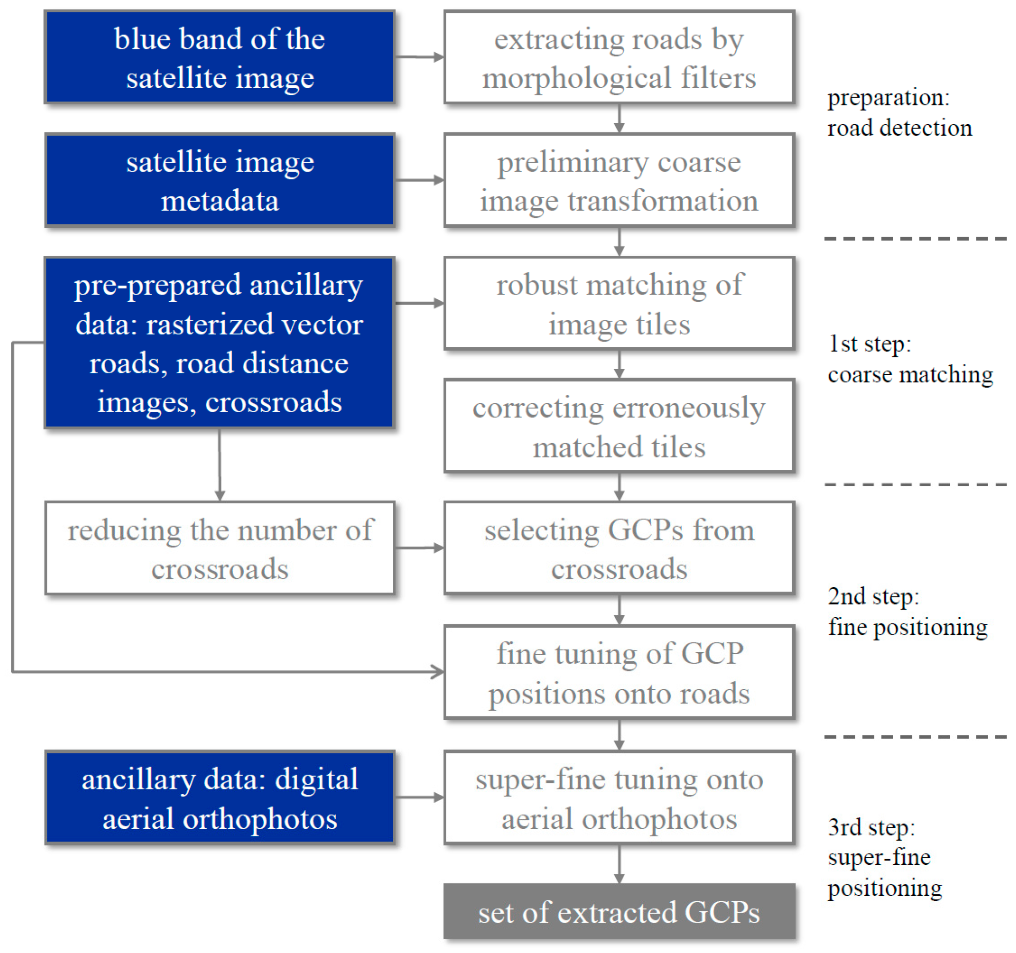
In order to overcome these issues the following three improvements were introduced to the GCP extraction algorithm (Figure 6): preliminary coarse image transformation, super-fine positioning onto the aerial orthophoto, and fixing GCPs candidates on the crossroads.

The issue with complex imaging geometry distortion was solved by adding coarse image transformation prior to the coarse matching. This preliminary transformation is based on the satellite image corner coordinates obtained from the accompanying metadata file. It is applied prior to all other image matching steps and ensures successful coarse matching. However, it does make the tracking and management of image pixel coordinates more complicated.

In order to overcome the problem of road widths an additional step was added to the original two-step algorithm: super-fine tuning of the positions by matching the GCP local vicinity on the input image to the national aerial orthophoto (Figure 5, right) with 0.5 m resolution and 1 m planar accuracy.

In the proposed solution the fine positioning onto the roads serves merely as a preparatory step for the super-fine positioning onto orthophotos. Although aerial orthophotos did not correlate to the entire image or tile in the coarse matching process (Section 3.1), they proved to be adequate for super-fine matching of small image-chips where merely a translation of a few pixels is anticipated. The translation parameters for super-fine matching of the GCP chip are defined by the maximisation of the correlation between pixel values I of the image-chip cropped from the perspectively corrected image and image-chip O cropped from the corresponding aerial orthophoto. The area of the image chip is denoted by S, and $\overrightarrow{s}={\left(s_x,s_y\right)}^T$ is a vector representing the current coordinate within the image chip. The correlation equation reads as follows:

$$C({\overrightarrow{r}}_0+\overrightarrow{\delta })=\text{\hspace{0.17em}\hspace{0.17em}\hspace{0.17em}}{\displaystyle \sum _{\overrightarrow{s}\in S}^{}I(\overrightarrow{s})\cdot O({\overrightarrow{r}}_0+\overline{\delta }+\overrightarrow{s})}\text{\hspace{0.17em}}$$

(1)

and the estimated GCP ground coordinate ${\overrightarrow{r}}_{}$ is found from the initial coarse estimate ${\overrightarrow{r}}_0$ once the maximum of the image correlation within a rectangular search window measuring 2∆ × 2∆ is established:

$$\overrightarrow{r}=\text{\hspace{0.17em}\hspace{0.17em}\hspace{0.17em}}{\overrightarrow{r}}_0+{\overrightarrow{\delta }}_{opt}\text{\hspace{1em}};{\overrightarrow{\delta }}_{opt}=\text{\hspace{0.17em}}\arg \underset{\begin{array}{l}{\delta }_x\text{}\in \left[-\Delta ,\Delta \right]\\ {\delta }_y\text{}\in \left[-\Delta ,\Delta \right]\end{array}}{\max }C({\overrightarrow{r}}_0+\overrightarrow{\delta })\text{\hspace{0.17em}}$$

(2)

Empirical tests have shown that the red band is optimal for super-fine positioning. Obviously, both chips have to be resampled to the same resolution, which should not differ too much from the satellite band resolution. In most cases a resolution of half of the satellite pixels was applied.

Another important addition to the previous algorithm was the decision to recruit GCP candidates as point features strictly on crossroads. On the other hand, roads as possible linear control features were not included in the matching process even when the number of crossroads was scarce. The crossroads were detected from the reference rasterized roads during the ancillary data preparation process and stored into a database. Every crossroad was equipped with coordinates in the reference coordinate system and an attribute numbering the road connections. As overpasses and ramps are scarce in this region, their existence was not checked. In order to lower the total processing time the set of all available crossroads was reduced depending on the satellite image resolution. Preferably crossroads with four road connections were used. This reduced set of crossroads presented the potential GCP locations. This ensured that each GCP candidate was firmly attached to a crossroad, which in turn, led to more accurate matching in the future processing. As a consequence, visual control of the entire process also became much easier. The final GCP candidate list included those crossroads that allowed for a successful detection and accurate matching. It is to be noted that VHR systems have smaller swath than HR systems, therefore the number of crossroads per WorldView-2 image is usually considerably smaller than on a RapidEye image. This may cause problems if some crossroads are not clearly detected, or if parts of an imaged area contain no crossroads at all.

3.3. Physical Sensor Model and Orthorectification

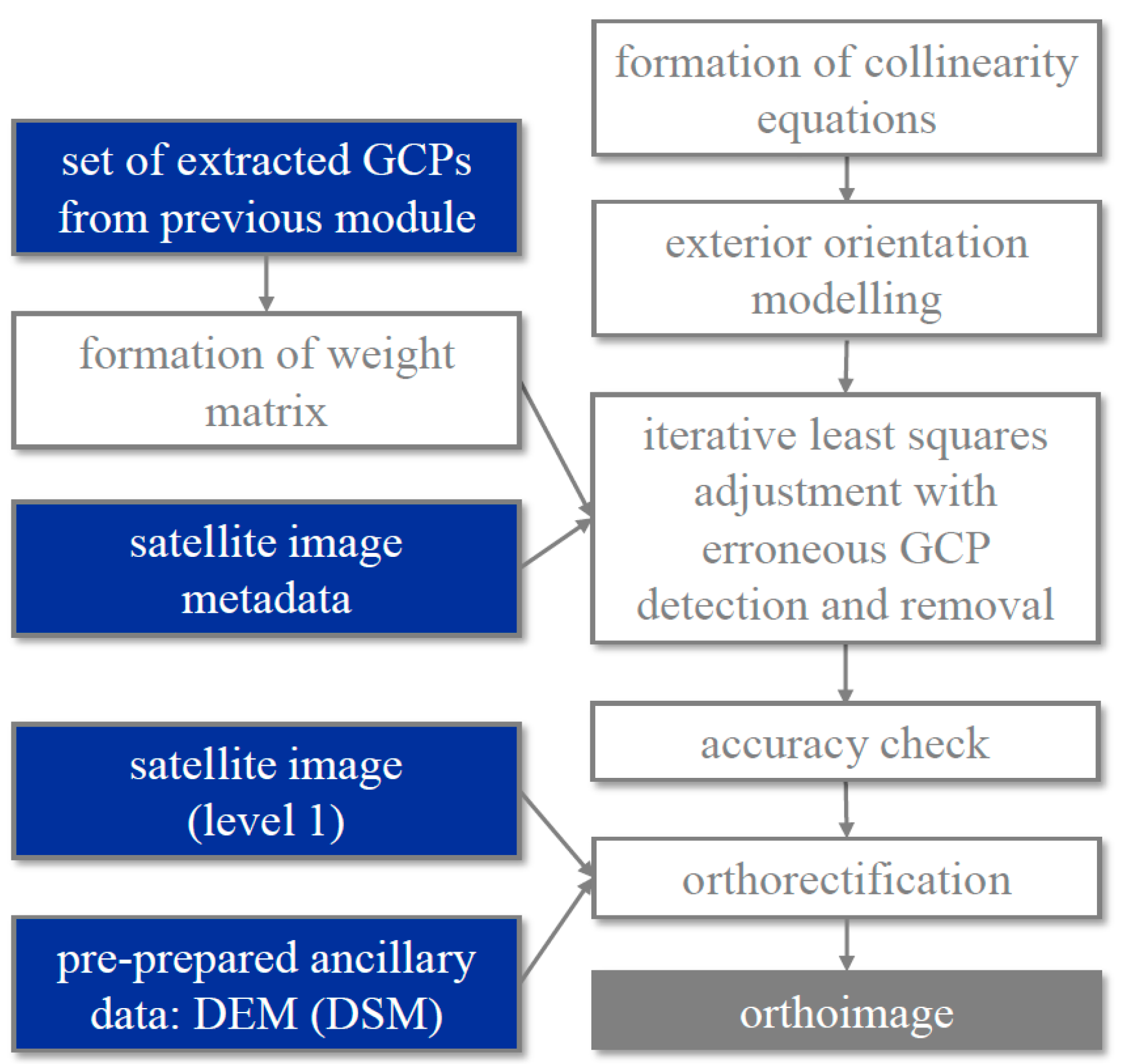
The automatic geometric corrections are implemented via two successive procedures: the first one includes sensor modelling, while the second one produces a GIS-ready image via orthorectification (Figure 3).

In order to accommodate various optical full-frame and pushbroom sensors a generic physical sensor model describing the exact sensor geometry during the acquisition was defined (Figure 7). The backbone of the developed model [24] is similar to the one described in [34], however numerous important changes have been made. The relationship between the platform and the ground system is represented by collinearity equations. In order to accommodate the complex pushbroom acquisition geometry the model uses 24 exterior parameters for sensor orientation. Due to the longer acquisition time the pushbroom sensor exterior orientation has to be modelled with time-dependent piecewise polynomial functions. The satellite orbit is divided into two segments. In each segment the exterior sensor orientation is modelled by six equations with 12 parameters in which three second-order polynomial equations depend on time t (Equation (3)):

$$\begin{array}{l}X(t)=\text{}{X}_0+X_{1}t+X_2{t}^2\\ Y(t)=\text{}{Y}_0+Y_{1}t+Y_2{t}^2\\ Z(t)=\text{}{Z}_0+Z_{1}t+Z_2{t}^2\\ \omega =\text{}{\omega }_0\\ \varphi =\text{}{\varphi }_0\\ \kappa =\text{}{\kappa }_0\end{array}$$

(3)

in which X, Y, and Z are position coordinates, while ω, φ, and κ are the attitudes of the platform in the reference (national) coordinate system. The smoothness of the orbit at the conjunction between adjacent segments is obtained by constraining the zero, first and second order continuity (derivatives) on the orbit functions. Therefore, the model can theoretically provide results with as little as six GCPs which should be spatially distributed as homogeneously as possible.

The initial approximations of the 24 unknown exterior parameters were obtained and calculated from the satellite image metadata. The final model was resolved using GCPs from the previous sub-module which defines the exact platform position and attitude during the image acquisition process. Prior to the iterative adjustment the GCP coordinates were corrected for systematic errors, which include Earth curvature and atmospheric refraction.

Blunder detection is an extremely important step within the sensor modelling process. Because the GCP extraction sub-module delivers some inaccurate GCPs or GCPs with gross errors, two methods—RANSAC [35] and robust estimation [36]—were utilized in order to detect and eliminate blunders in the sensor model. For this reason, the sensor model was divided into two parts that combined least squares adjustment with gross error detection. Firstly, RANSAC was used to remove GCPs with large errors, and then the model was optimized with robust estimation. In our algorithm we implemented the Klein method [37].

The orthorectification of pushbroom images was performed with an indirect method based on the research conducted by Kim et al. [38]. Relief displacement was corrected pixel by pixel by computing the correct pixel’s position within the orthoimage with the aid of a nationwide DEM with a resolution of 12.5 m and an estimate of the satellite sensor parameters.

3.4. Rational Function Model and Orthorectification

The physical sensor model was also tested on WorldView-2 imagery. The WorldView-2 metadata file has a different format and types of parameters to the RapidEye metadata file, therefore the algorithm for the extraction and computation of the first approximations of unknown parameters was adapted while the model itself was left unchanged. The model yielded accurate results if there was a sufficient number of homogeneously distributed GCPs (see Section 5.4). Since this was rare—some possible reasons are outlined in Section 3.2—the RFM was also introduced to our processing chain as a complement to the physical sensor model. The RFM provides a good alternative to the physical model and can achieve equivalent results [39]. In our case the RFM (performed with vendor-provided RPCs) was less sensitive to the number and distribution of GCPs than the physical sensor model which—because of its generality—does not model appropriately all sensor-specific distortions (e.g., lens, detector, asynchronous mode) that are important for VHR sensors. The bias correction of RPCs needs a substantially lower number of GCPs, which do not need to be evenly distributed. The self-evident requirement for the use of this model is that the satellite image metadata includes RPCs, which is not always the case.

The RFM uses a ratio of two polynomial functions to compute the row and column image coordinates (r, c) from the object space ground coordinates (usually φ, λ, h). In order to minimize the introduction of errors during the calculations, all of the coordinates and coefficients are normalized. The ratios of the polynomials for the transformation of the coordinates from the ground to the image can be calculated as follows (Equation (4)) [40]:

$$\begin{array}{l}{r}_n=\frac{{\displaystyle \sum _{i=0}^{m1}{\displaystyle \sum _{j=0}^{m2}{\displaystyle \sum _{k=0}^{m3}{a}_{ijk}{P}^i{L}^j{K}^k}}}}{{\displaystyle \sum _{i=0}^{n1}{\displaystyle \sum _{j=0}^{n2}{\displaystyle \sum _{k=0}^{n3}{b}_{ijk}{P}^i{L}^j{K}^k}}}}\\ c_n=\frac{{\displaystyle \sum _{i=0}^{m1}{\displaystyle \sum _{j=0}^{m2}{\displaystyle \sum _{k=0}^{m3}{c}_{ijk}{P}^i{L}^j{K}^k}}}}{{\displaystyle \sum _{i=0}^{n1}{\displaystyle \sum _{j=0}^{n2}{\displaystyle \sum _{k=0}^{n3}{d}_{ijk}{P}^i{L}^j{K}^k}}}}\end{array}$$

(4)

in which r_n and c_n are the normalized row and column image coordinates, P, L, and H are the normalized ground coordinates (φ, λ, and h, respectively), while a_ijk, b_ijk, c_ijk, and d_ijk represent the RPCs. The satellite image vendors usually supply 20 RPCs for polynomials in both numerators and denominators, consequently the maximum and total power of all ground coordinates (m1, m2, m3, n1, n2, n3) is limited to three.

The RFM is simple and straightforward to implement but one still needs at least a few GCPs to obtain accurate results, since RPCs are usually precise but have to be bias-corrected first. The correction is performed with all of the extracted GCPs. The GCPs are introduced into the model and the obtained residuals of each individual GCP are used to compute the coefficients of two first order polynomials (one for each image coordinate) which are later used to correct the pixel positions during orthorectification. The algorithm also uses a simple gross error detection procedure. This eliminates the GCPs the residuals of which differ by over 2σ from the mean value. Using RPCs and the correction coefficients the image is orthorectified in the reference coordinate system with the use of the indirect method.

4. Test Data and Accuracy Evaluation Measures

4.1. Test Data

The robustness, speed, reliability and accuracy of the developed algorithms were tested with HR RapidEye images and VHR multispectral WorldView-2 images.

The available RapidEye imagery (resolution 6.5 m) consisted of two different datasets of 41 level 1B images (

Table 1. Selected characteristics and metadata parameters for 41 RapidEye level 1B images. Images are referenced by dates.

Image	Season	No. of Samples	No. of Lines	Image Size	Clouds (%)	Sun Elevation (°)	Off-Nadir Angle (°)	Snow Coverage	Imaged Landscape
13.12.2010	autumn	11807	7623	standard	6	20.4	0.4	partially	lowlands
27.12.2010	autumn	11788	7605	standard		20.3	6.6	partially	lowlands
03.02.2011	winter	11810	7447	standard	2	27.0	−16.2	partially	lowlands
11.03.2011	winter	11727	7523	standard		39.8	−9.5	sporadic	lowlands
03.05.2011	spring	11839	7631	standard	6	59.3	0.4		lowlands
12.05.2011	spring	11730	7568	standard	13	61.6	−6.4		lowlands
11.06.2011	spring	11802	7604	standard		66.6	3.6		lowlands
07.07.2011	summer	11797	7594	standard	1	66.1	−3.2		lowlands
11.08.2011	summer	11841	7612	standard		58.9	0.4		lowlands
14.08.2011	summer	11792	7590	standard		57.9	3.4		lowlands
15.08.2011	summer	11738	7582	standard	12	57.6	0.6		lowlands
02.09.2011	summer	11792	7622	standard		51.6	0.1		lowlands
13.09.2011	summer	11730	7554	standard	4	47.3	−9.7		lowlands
01.08.2013	summer	11802	11223	large	3	61.7	0.1	partially	mountains
06.03.2011	winter	11724	7616	standard		38.8	10.4		coastal
09.03.2011	winter	11790	7571	standard	1	38.9	19.5		lowlands
11.03.2011	winter	11727	7523	standard		39.7	−9.5	sporadic	lowlands
11.03.2011	winter	11729	7522	standard		40.2	−9.5	sporadic	lowlands
11.03.2011	winter	11730	7532	standard	2	41.0	−9.5	partially	lowlands
12.03.2011	winter	11796	7550	standard	1	40.1	20.3	sporadic	lowlands
20.03.2011	winter	11719	7578	standard	3	43.1	13.8	sporadic	hills
20.03.2011	winter	11719	18078	ext. large	9	44.0	13.8	sporadic	hills
02.04.2011	spring	11815	7515	standard	22	48.4	−12.9		lowlands
03.04.2011	spring	11806	7436	standard	4	49.0	−16.2		lowlands
03.04.2011	spring	11804	7433	standard	1	49.6	−16.2		lowlands
20.04.2011	spring	11855	25069	ext. large	3	55.7	3.8	partially	mixed
22.04.2011	spring	11787	7558	standard	9	56.1	3.4	partially	mountains
06.05.2011	spring	11787	9246	large	6	60.3	13.3	partially	mountains
07.05.2011	spring	11723	13368	large	1	60.7	3.5	sporadic	hills
07.05.2011	spring	11723	8322	standard		61.4	3.5	sporadic	hills
07.05.2011	spring	11723	9322	large		61.5	3.5	sporadic	hills
12.05.2011	spring	11727	8589	standard	10	62.3	−6.4		lowlands
26.05.2011	spring	11726	9979	large	4	64.9	10.3	partially	mountains
26.05.2011	spring	11724	8563	standard	1	65.7	10.3		coastal
11.06.2011	spring	11801	12826	large		66.5	3.6		lowlands
16.06.2011	spring	11800	10091	large	1	68.0	−3.1		lowlands
23.06.2011	summer	11795	7586	standard	6	68.2	−6.4		coastal
07.07.2011	summer	11797	7595	standard	1	66.3	−3.2		lowlands
07.07.2011	summer	11795	8578	standard	2	66.6	−3.2		lowlands
07.07.2011	summer	11795	8587	standard	6	66.8	−3.2		lowlands
07.07.2011	summer	11794	7603	standard	10	67.1	−3.2		lowlands

).

The primary source was represented by 14 images, thirteen of which represented a time series of the same lowland area acquired on different dates and in different seasons in 2010 and 2011, thus exposing different illumination and vegetation characteristics, while the fourteenth image was acquired in 2013 and covered a mountainous area. A more heterogeneous set of 27 images acquired in 2011 represented an additional data source. This dataset was obtained within the frame of the Copernicus Space Component Data Access (dataset name “DWH_MG2_CORE_01—Optical HR Pan EU coverages 2011/2012/2013”) [41] and presents full coverage of Slovenia, thus encompassing the full variety of landscapes (lowlands, hills, mountains, and coastal) during a five month period. The high variability of input RapidEye images from both datasets is shown in Table 1.

The available multispectral WorldView-2 imagery (with a resolution of approximately 2 m) was acquired in 2010 and 2012 (

Table 2. Selected characteristics and metadata parameters for nine WorldView-2 level 1B and 2A images. The variability of the available WorldView-2 images is smaller than that of RapidEye images. Images are referenced by location names.

Image	Proc. Level	Season	No. of Samples	No. of Lines	Image Size	Clouds [%]	Sun Elevation [°]	Off-Nadir Angle [°]	Imaged Landscape
Jesenice	1B	summer	8472	7415	standard	3	47.6	12.8	mountains
Bled	1B	summer	8464	7409	standard	5	47.7	12.5	hills
Ljubljana L	1B	summer	8766	7603	standard		59.0	18.8	lowlands
Ljubljana S	1B	summer	8762	3106	small		59.1	18.7	lowlands
Puconci	2A	spring	4999	7112	standard	n.a.	66.2	31.2	lowlands
Radenci	2A	spring	4999	4999	standard	n.a.	66.2	30.6	lowlands
Ljutomer	2A	spring	7191	4999	standard	n.a.	66.0	28.8	lowlands
Lendava	2A	spring	9998	4999	standard	n.a.	66.1	28.8	lowlands
Šentjernej	2A	spring	4998	9997	small	n.a.	66.4	16.6	lowlands

). Four images (Jesenice, Bled, Ljubljana L and smaller Ljubljana S) are level 1B (sensor-corrected), while the other five are level 2A ortho-ready. The Jesenice and Bled images present a more dynamic landscape including hills and mountains, while the remaining seven present lowland areas. No winter WorldView-2 image was available.

4.2. Accuracy Evaluation Measures

The implemented geometric corrections were evaluated from the perspective of all target requirements. At this point a short introduction is given for a better understanding of the accuracy evaluations (used measures are summarized in

Table 3. Used accuracy evaluation measures. RMSE is root-mean-square error. RPCs are rational polynomial coefficients. Ground control points (GCPs) were automatically extracted. Independent check points (ICPs) and "orthoimage ICPs" (OICPs) were manually digitized from satellite image and national aerial orthophotos.

Evaluated Property and Processing Phase	Evaluation Measure	Number of Used Images
accuracy of sub-module for automatic GCP extraction	RMSE at bias-corrected RPCs for all extracted GCPs	41 RapidEye 9 WorldView-2
accuracy of sensor model	model RMSE at non-eliminated GCPs and ICPs	14 RapidEye 3 WorldView-2
sensitivity of sensor model on number of GCPs	model RMSE at reduced subsets of non-eliminated GCPs and ICPs	3 WorldView-2
accuracy of the output orthoimage	RMSE at OICP	3 WorldView-2

). All main processing steps (see Figure 3) were tested separately.

The accuracy of the GCP extraction algorithm—regardless of whether it is a two- or three-step one—was evaluated through the comparison of the positions of all extracted GCPs with the positions calculated from bias-corrected RPCs (Section 5.2 and Section 5.3). Therefore, we could say that in this evaluation step RPCs were used as a reference source, however we were fully aware that they do not represent a perfect reference. Due to this the final RMSEs might contain certain small errors, however, in our experience, these do not have a great effect on the evaluation results.

Secondly, the accuracy of the physical sensor model for processing HR and VHR images was evaluated with respect to the manually measured ICPs and GCPs via the computed model parameters (Section 5.4). In this case only the GCPs that were not eliminated by RANSAC were taken into account. Total RMSEs were calculated for all non-eliminated GCPs as well as for the ICP sets.

In order to verify the influence of the number of GCPs on the sensor model algorithm the same assessment was performed on the artificially produced subsets of non-eliminated GCPs (for VHR images only).

Finally, the accuracy of the final output VHR orthoimages was assessed by a comparison with an external reference source (Section 5.4). Approximately 30 manually selected “orthoimage ICPs” (OICPs) placed on road intersections were manually digitized. The coordinates of the same locations were taken from national aerial orthophoto images. The orthorectification accuracy (OICP RMSE) was computed from the coordinate differences. It should be pointed out that the OICPs were measured only on well-defined road intersections predominantly located on plain lowlands.

The accuracy of the RFM and the orthorectification sub-module for processing VHR images was assessed with the same measures that were used for the physical sensor model and the orhorectification sub-module; the results are presented in Section 5.5.

5. Results

5.1. Robustness and Processing Time of Geometric Corrections

The two-step GCPs extraction algorithm automatically processed 40 out of the total 41 RapidEye images (i.e., 97.6%). All 40 images that successfully completed the automatic GCP extraction also passed the physical sensor model and were automatically orthorectified.

An average per-image processing time for the entire geometric correction phase lasted 41 minutes on a personal workstation (quad-core, 3.40 GHz, 16 GB RAM). The largest image (“20.04.2011”), which is the size of three standard images, was processed in 1 h 42 min, which is still acceptable for such an extraordinary large image. Approximately 35% of the processing time is dedicated to GCP extraction, 5% to the sensor model, and 60% to the orthorectification.

All nine WorldView-2 multispectral images were fully automatically geometrically corrected via the three-step GCP extraction algorithm and the physical sensor model or RFM, with processing times under one hour. When the physical sensor model was used individual steps took around 28%, 7%, and 65%, respectively, while with RFM the second step was performed in mere seconds.

While the number of WorldView-2 images is rather low for a definite conclusion, the rate and processing times of the automatically processed RapidEye images implies great robustness and speed of the implemented algorithms.

5.2. Evaluation of the Automatic Two-Step GCP Extraction Algorithm

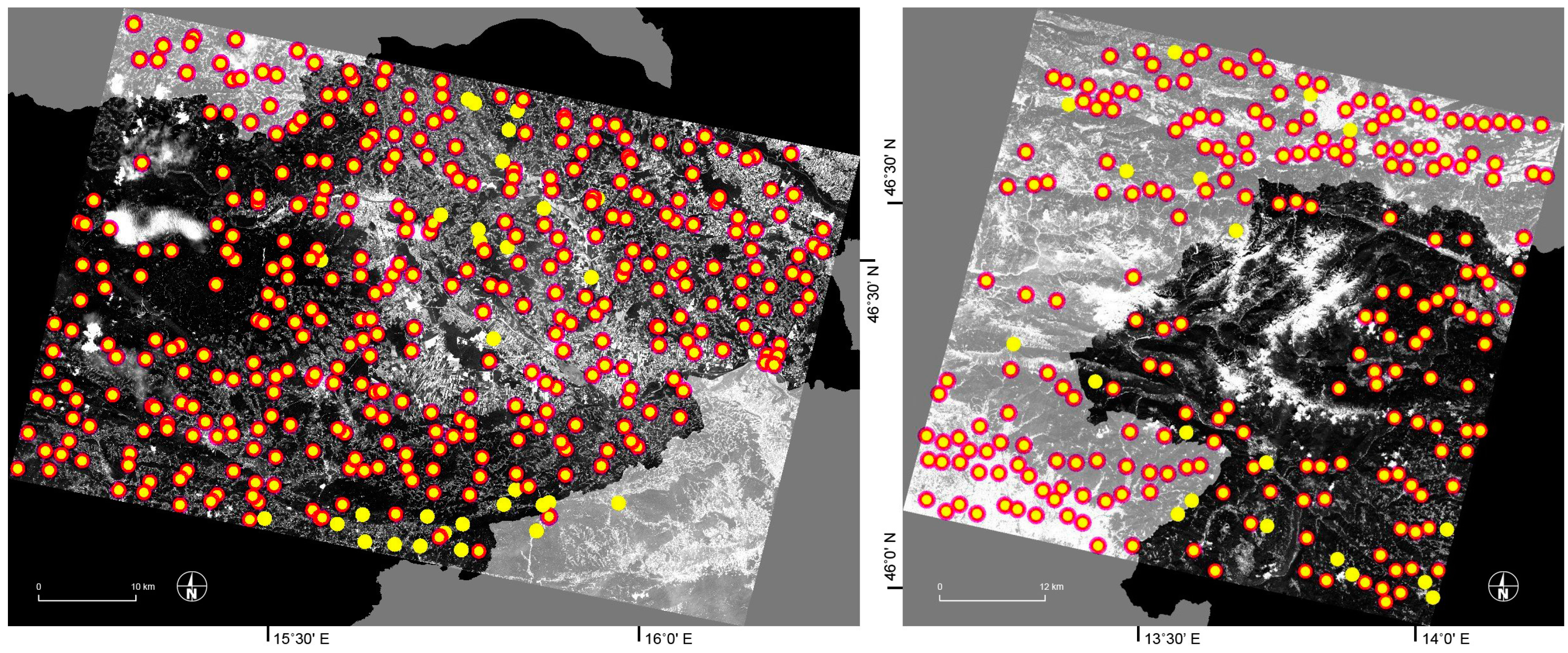
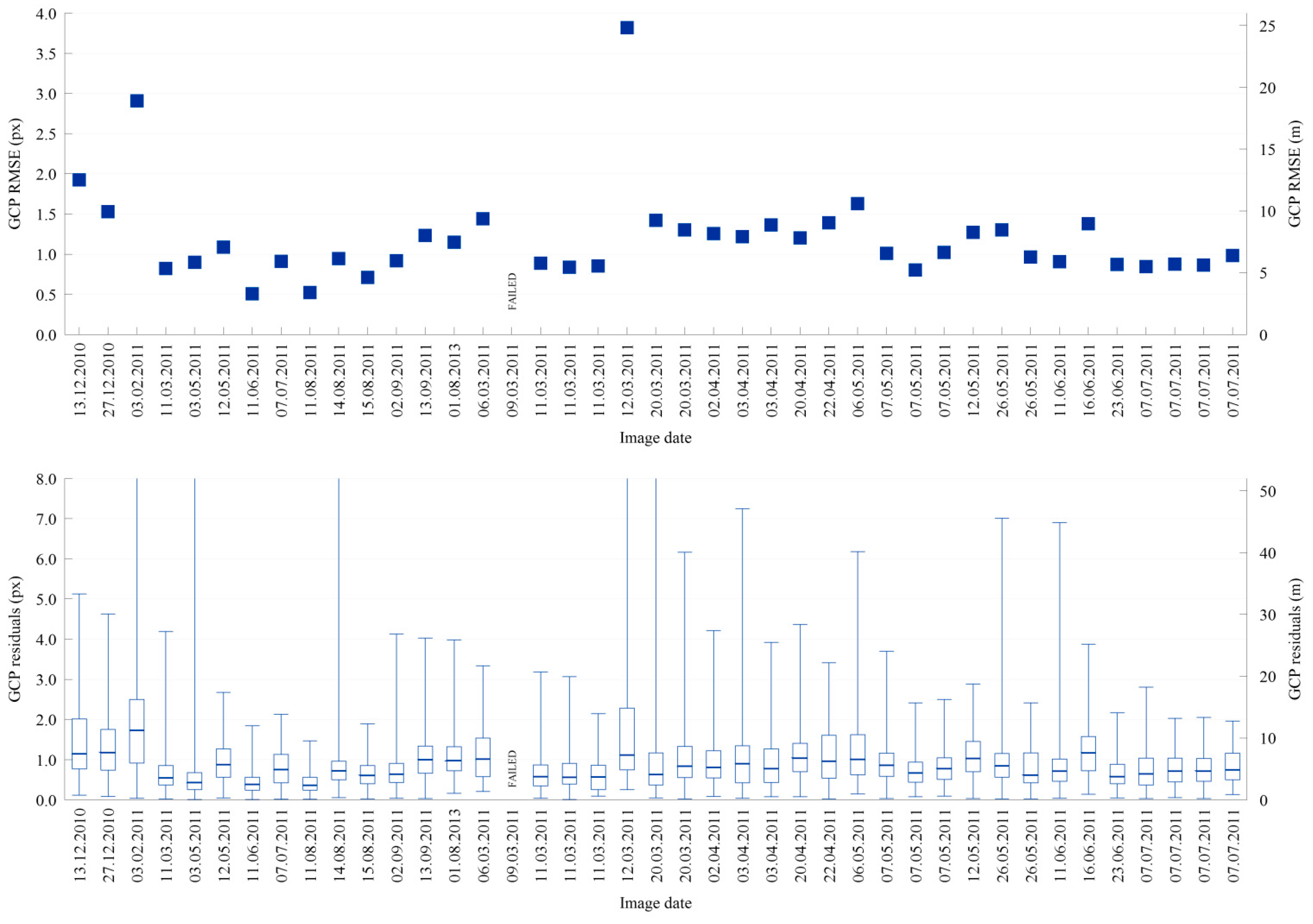
The algorithm typically extracts 200–300 GCPs per RapidEye image, however when dealing with complex images (clouds, snow) in which the internal evaluation of the GCP quality prevents the extraction of unreliable GCPs, or if the imaged area is poorly covered by a road network, this number can be lower, even as low as 50. The distribution of GCPs (Figure 8) and their positions were visually inspected, while the accuracy of the GCPs was evaluated via the bias-corrected RPCs. The per image root-mean-square error (RMSE) calculated at extracted GCPs and the boxplots of GCP residuals are presented in Figure 9. The average RMSE value of all 40 successfully processed images is 1.19 px.

When compared to Table 1 we may see that images with RMSEs larger than average were acquired in challenging conditions, i.e., winter (presence of snow, lower contrasts and longer shades), mountainous terrain and/or large across-track angle. For images extending across the Slovenian borders we had a problem with the absence of a reliable reference road source.

When dealing with images acquired in non-challenging conditions 75% percent of residuals remain within 1.3 pixels, while individual residuals may reach as high as two to ten pixels. Residuals may be higher for images acquired in challenging conditions. GCPs with gross errors are removed in the sensor model processing step (see Section 3.3 and Section 3.4).

5.3. Evaluation of the Automatic Three-Step GCP Extraction Algorithm

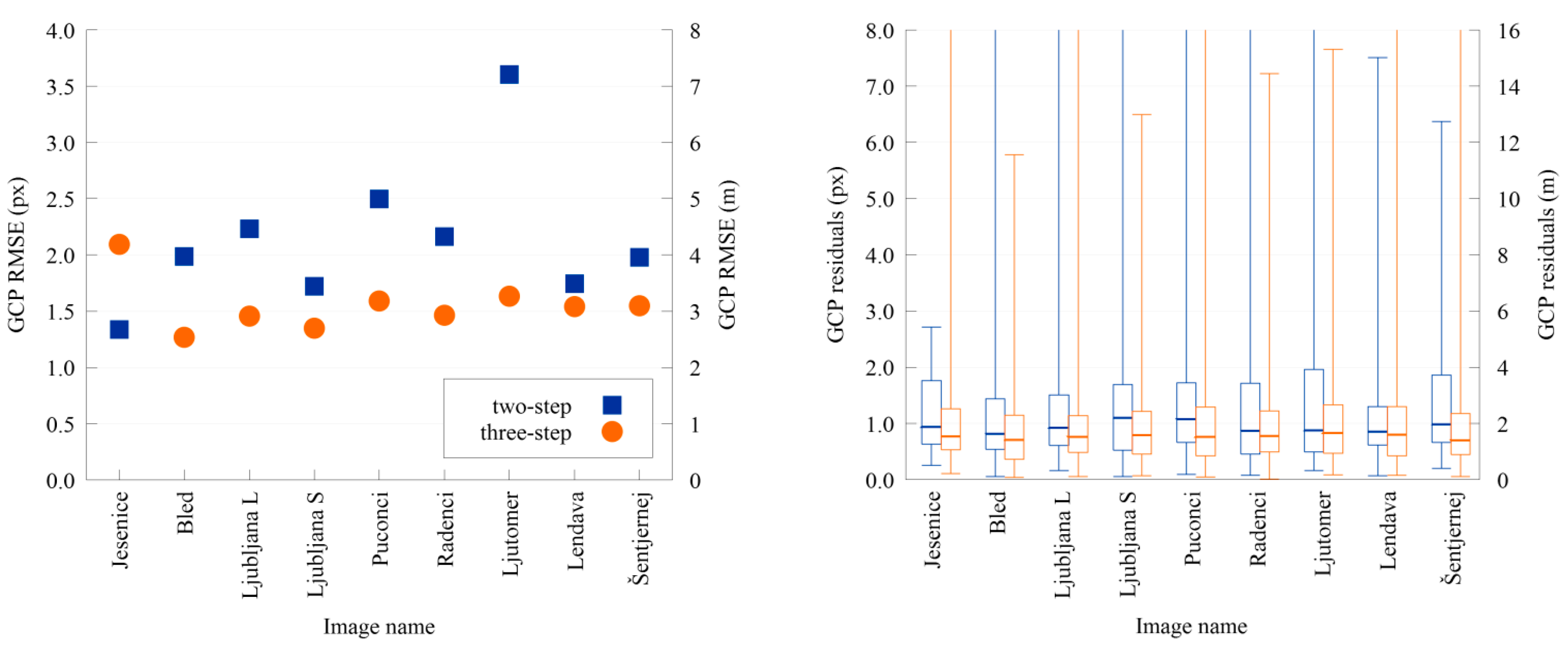
In most cases the algorithm extracted over 100 GCPs per image. The average RMSE for the extracted GCPs in nine WorldView-2 images was 1.55 px (Figure 10, left). For comparison, the same images were processed by the original two-step algorithm with an average RMSE of 2.14 px.

In the two-step algorithm 75% percent of GCP residuals stay within two pixels for all images (Figure 10, right). Individual residuals do not exceed five pixels on a single image. Once the three-step algorithm is used 75% residuals remain within 1.5 pixels, which is a substantial improvement. On the other hand, individual residuals remain high. Individual GCPs with gross errors are removed in the sensor model processing step (see Section 3.3 and Section 3.4).

5.4. Evaluation of the Physical Sensor Model and Orthorectification

The physical sensor model was tested with RapidEye and multispectral WorldView-2 images. The tests with three RapidEye images were extensively presented in [24]. The results showed that the model is capable of orthorectifying optical satellite images with an accuracy of under one pixel even when less than 20 GCPs are used and several gross errors of different magnitudes are present. In order to support these findings 14 RapidEye 1B images were analysed (primary image set, see Section 4.1). The results presented in

Table 4. Root-mean-square error (RMSE) values for 14 RapidEye level 1B images processed with the physical sensor model. The number of GCPs was reduced by RANSAC and further refined by robust estimation. Independent check points (ICPs) were manually digitized.

Image	Number of Total GCPs	Number of Used GCPs	GCP RMSE (px/m)	ICP RMSE (px/m)
13.12.2010	55	49	0.79/5.14	0.55/3.58
27.12.2010	89	81	0.92/5.98	1.19/7.74
03.02.2011	106	96	1.15/7.48	0.94/6.11
11.03.2011	329	328	0.74/4.81	0.74/4.81
03.05.2011	253	246	0.56/3.64	0.57/3.71
12.05.2011	270	257	0.77/5.01	0.64/4.16
11.06.2011	327	304	0.57/3.71	0.80/5.20
07.07.2011	410	401	0.59/3.84	0.83/5.40
11.08.2011	126	115	0.49/3.19	0.47/3.06
14.08.2011	369	336	0.67/4.36	0.94/6.11
15.08.2011	377	347	0.42/2.73	0.58/3.77
02.09.2011	237	223	0.50/3.25	0.56/3.64
13.09.2011	269	262	1.04/6.76	0.69/4.49
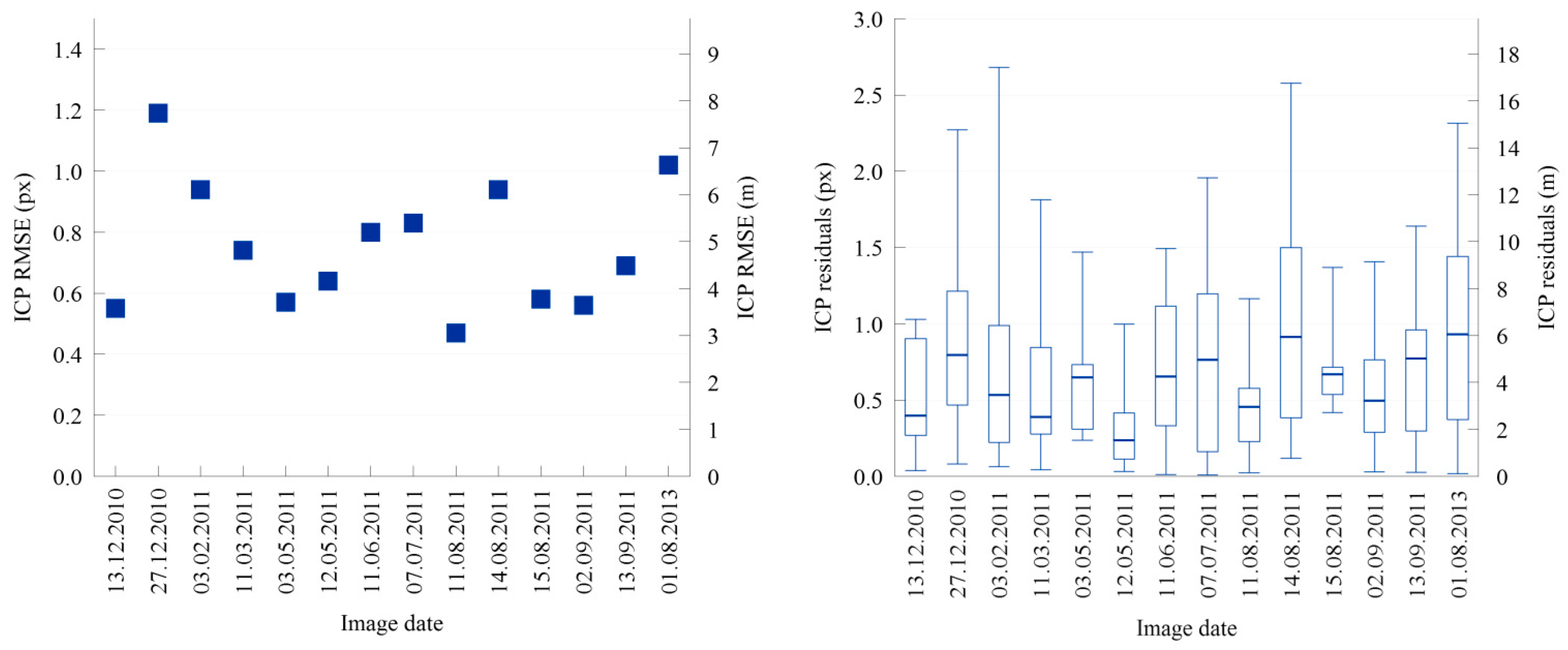
01.08.2013	184	166	0.63/4.10	1.02/6.63

and Figure 11 (left) show that the total RMSE of the non-eliminated GCPs and the RMSE of independent check points (ICPs) are in most cases far below one pixel, which is in line with the results in [24]. ICP residuals (Figure 11, right) reflect the RMSE values. 75% of residuals are below 1.5 pixels for all images. Only four images, mostly winter and mountainous, have residuals that exceed two pixels.

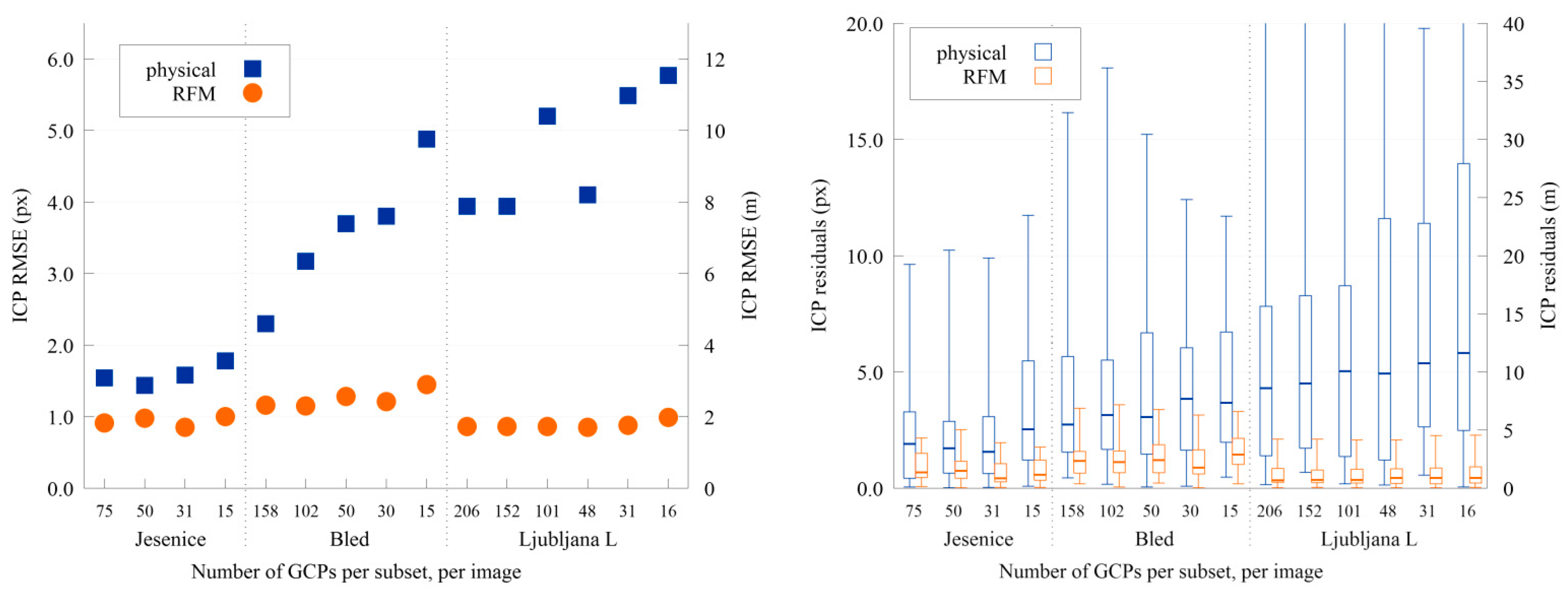
We had only three full-size 1B multispectral WorldView-2 images available for testing. In order to increase the number of tests that would determine the model efficiency, the original set of GCPs extracted from previous sub-module was decimated according to the GCP accuracy and distribution and with this process we formed several subsets with different numbers of GCPs. Each subset was used in the sensor model that worked with 300 RANSAC iterations. The RANSAC iterations continued until at least 90% of the GCPs remained in the set. Since RANSAC has a random component and the results tend to differ slightly in each test (same set of GCPs of the same image) the test was conducted five times and the results were averaged.

The adjustment results are listed in

Table 5. Accuracy of the adjustment results obtained with the physical sensor model on different subsets of automatically extracted GCPs for three multispectral WorldView-2 1B images.

Image	Number of Total GCPs	Number of Used GCPs	Number of ICPs	GCP RMSE (px/m)	ICP RMSE (px/m)
Jesenice	75	70	24	0.92/1.84	1.54/3.08
	50	48	24	1.17/2.34	1.44/2.88
	31	28	24	0.98/1.96	1.58/3.16
	15	14	24	0.74/1.48	1.78/3.56
Bled	158	149	30	0.99/1.98	2.30/4.60
	102	97	30	1.11/2.22	3.17/6.34
	50	47	30	1.15/2.30	3.70/7.40
	30	29	30	1.35/2.70	3.80/7.60
	15	14	30	0.88/1.76	4.88/9.76
Ljubljana L	206	191	30	2.61/5.22	3.94/7.88
	152	145	30	2.85/5.70	3.94/7.88
	101	92	30	3.05/6.10	5.20/10.40
	48	45	30	3.06/6.12	4.10/8.20
	31	29	30	3.33/6.66	5.49/10.98
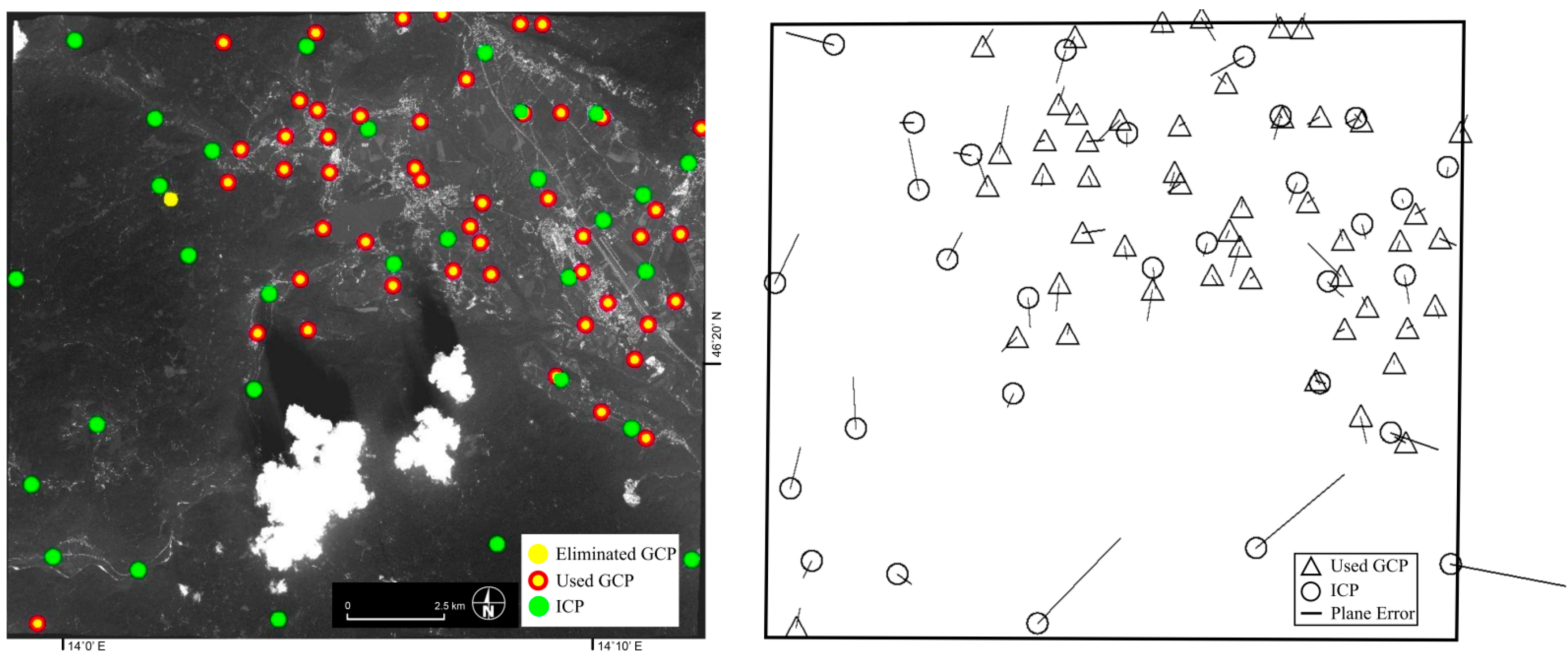
	16	15	30	2.97/5.94	5.77/11.54

. It can be noted that RANSAC always removed at least 5% of the points in every set. Following the adjustment, the RMSE was computed from the difference between the measured and computed coordinates. The RMSEs at manually measured ICPs, which are more significant than internal RMSEs at GCPs, exceed one pixel for every configuration and as much as five pixels when fewer points are used in the Ljubljana L image. It is to be noted that although the GCP RMSE values reflect the obtained GCP accuracies when compared to RPCs, the RMSEs at ICPs are higher. The reason for this lies in the GCPs number and distribution (Figure 12). The physical model showed to be quite sensitive to the number of available GCPs and their spatial distribution.

The orthoimages were automatically generated with the computed parameters from the most accurate results of all subsets (with the lowest ICP RMSE) and a nationwide DEM. The accuracy of the orthoimages was assessed with manually selected OICPs as described in Section 4.2.

Table 6. Accuracy of the WorldView-2 orthoimages generated with the physical model compared to the reference aerial orthophoto.

Image	Number of OICPs	OICP RMSE (px/m)
		X	Y	Planar
Jesenice	30	0.80/1.60	0.84/1.68	1.16/2.32
Bled	32	0.69/1.38	1.78/3.56	1.91/3.82
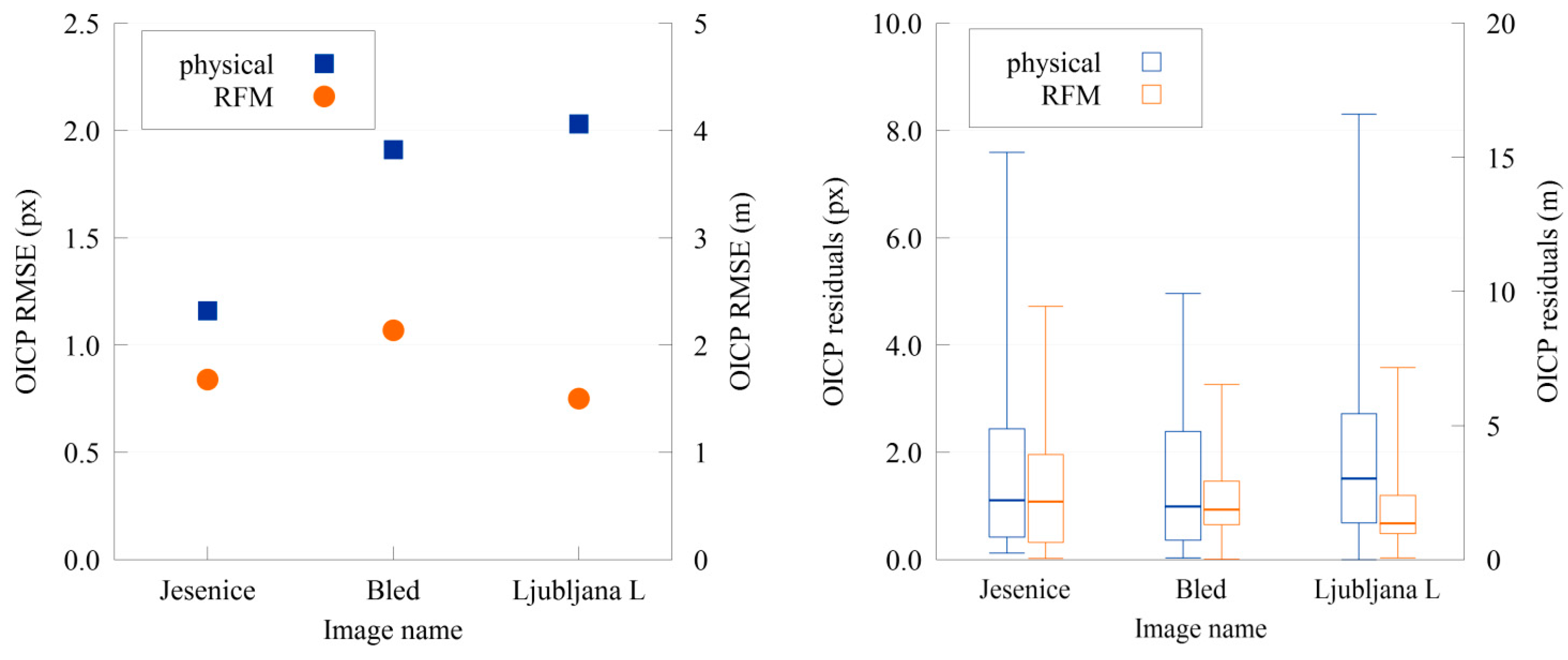
Ljubljana L	32	1.03/2.06	1.75/3.50	2.03/4.06

shows the positional accuracy of the orthoimages. The resulting OICP RMSE is approximately two pixels for the Bled and Ljubljana L image and just over one pixel for the Jesenice image. The accuracies are better than that of ICPs after the adjustment (Table 5).

5.5. Evaluation of the RFM and Orthorectification

The same images and GCP sets were used for RFM and the physical sensor model. The results of the tests for the three WorldView-2 1B images are presented in

Table 7. Accuracy of the results obtained with RFM on different subsets of automatically extracted GCPs for three multispectral WorldView-2 1B images.

Image	Number of Total GCPs	Number of Used GCPs	Number of ICPs	GCP RMSE (px/m)	ICP RMSE (px/m)
Jesenice	75	69	24	0.88/1.76	0.91/1.82
	50	47	24	1.01/2.02	0.98/1.96
	31	28	24	1.04/2.08	0.85/1.70
	15	13	24	0.77/1.54	1.00/2.00
Bled	158	147	30	0.86/1.72	1.16/2.32
	102	94	30	0.94/1.88	1.15/2.30
	50	46	30	0.87/1.74	1.28/2.56
	30	28	30	0.92/1.84	1.21/2.42
	15	13	30	0.79/1.58	1.45/2.90
Ljubljana L	206	189	30	0.93/1.86	0.86/1.72
	152	140	30	0.93/1.86	0.86/1.72
	101	91	30	0.95/1.90	0.86/1.72
	48	44	30	0.89/1.78	0.85/1.70
	31	28	30	0.94/1.88	0.88/1.76
	16	15	30	1.05/2.10	0.99/1.98

. The number of eliminated GCPs is similar to that of the physical sensor model. The total RMSE of the used non-eliminated GCPs and RMSE of ICPs are in most cases less than one pixel. Compared to other images the Bled image shows rather larger errors in ICPs. In general, the results obtained with RFM are substantially better than the results obtained with the physical model (Figure 13, left). ICP residuals (Figure 13, right) also support these findings. In the case of the RFM model the maximum residuals remain within 3.5 pixels for all images while the median rarely exceeds one pixel. On the other hand, the physical model presents larger residuals, with median values exceeding five pixels.

The orthoimages were generated using bias-corrected RPCs of the most accurate subset and a nationwide DEM. The accuracy of the orthoimages was assessed as described in Section 4.2.

The positional accuracies of the orthoimages can be seen in

Table 8. Accuracy of the WorldView-2 orthoimages generated with RFM compared to the reference aerial orthophoto.

Image	Number of OICPs	OICP RMSE (px/m)
		X	Y	Planar
Jesenice	30	0.58/1.16	0.61/1.22	0.84/1.68
Bled	32	0.43/0.86	0.98/1.96	1.07/2.14
Ljubljana L	32	0.42/0.84	0.62/1.24	0.75/1.50

. The resulting OICP RMSEs reflect the results obtained with RFM (Table 7). The precision of the orthoimages is even better, with RMSEs below one pixel for Jesenice and Ljubljana L images and slightly over one pixel for the Bled image. In the case of orthoimages the results obtained with RFM are also better than the results obtained with the physical model (Figure 14, left). The orthophoto residuals (Figure 14, right) generated with the RFM model are smaller than the ones generated with the physical model. Their median remains below one pixel and merely a few residuals exceed three pixels. The physical model residuals have a similar median but are in general larger and reach higher maximums. On two images, certain areas present residuals above six pixels. Apart from the model’s imperfections, the high residuals are also a result of the low accuracy of the used aerial orthophoto and DEM in hilly and mountainous areas.

6. Discussion

As regards the processing times and robustness the STORM processing chain meets the target requirements for HR and VHR images.

With the two-step algorithm delivering a sufficient number of GCPs with an average accuracy of 1.18 px on heterogeneous HR RapidEye images, we consider that we are getting close to the limitations of a fully automatic GCP extraction method. The accuracies of the three images with complex acquisition parameters (“03.02.2011”, “09.03.2011”, “12.03.2011”) are notably lower than the average. All of these three images were taken during winter and were acquired with large across-track viewing angles (more than 16°). Moreover, most of the second listed image (from which an insufficient number of GCPs was extracted) lies outside of Slovenia, while the first one is so complex that even manually selecting accurate ICPs proved to be a demanding task. It may be concluded that a combination of several acquisition parameters that are too far from the common or expected values may hinder the fully automatic execution of the proposed algorithm.

It was established that the algorithm was able to withstand imperfect road detection on satellite images as well as roads missing in source reference layers. Coarse image matching was almost entirely successful wherever digital road data was available and where a sufficient part of the road network was visible on the satellite image. The road density derived from the available road layers in Slovenia was larger than that in the neighbouring countries where OpenStreetMap was used; there the method yielded a smaller—in some cases insufficient—local number of GCPs. An insufficient number of local GCPs was also recorded in mountainous areas. The GCP extraction algorithm was also challenged if the satellite image was acquired with a large across-track viewing angle.

The three-step algorithm delivers large sets of accurate GCPs on VHR WorldView-2 images. For the nine images the average bias-corrected RPC RMSE of extracted GCPs was 1.55 px. Such accuracy was achieved by adding correlation-based super-fine positioning in the final step, however, we believe there is still room for further refinements. Two types of improvements are possible. In the first one, the implemented super-fine matching method could be replaced or supplemented by a different algorithm, e.g., least square matching or speeded up robust features. Its performances should be compared to the algorithms found in literature. In the second type, certain criteria function(s) could be developed that would eliminate the worst extracted GCPs, thus reducing their redundancy and resulting in improved overall accuracy. Nevertheless, it is not expected that the pixel accuracy of GCPs extracted from VHR images will ever reach those from HR images. The reason for this lies in the detail complexity and local distortions (deformations of high objects, objects’ shadows) that are a result of the imaging geometry which is extremely pronounced in VHR images.

The number of GCPs and their distribution on VHR images is not always acceptable. Due to the smaller swath some parts of the VHR image may contain no roads at all (e.g., mountainous areas, extensive forest areas), thus not a single GCP can be extracted. In this case it would be beneficial to use a complementary GCP extraction method, which would use a different reference source and not roads. Both two- and three-step GCP extraction algorithms produce some GCPs with gross errors. They were removed during the following processing step, i.e., the sensor model.

The sensor model and the orthorectification sub-module of the STORM processing chain was able to produce HR and VHR orthoimages either with the proprietary physical sensor model or with RFM based on previously extracted GCPs which were used to compute the orientation parameters or correct the RPCs.

The physical sensor model was first tested on 14 HR RapidEye images. The obtained ICP RMSEs were almost always below one pixel, even in the case of the three winter images. Nevertheless, the winter images and the image of the mountainous area from 2013 have proven to be the most problematic. The number of GCPs does not drastically affect the results as the same accuracies are achieved with over 400 or as few as 50 points. As it was demonstrated in [24] the physical model is stable and immune to the presence of gross errors.

The physical sensor model applied on VHR WorldView-2 images represented a greater challenge. From the three test images only one (Jesenice) performed well on all evaluated levels, with GCP RMSE, ICP RMSE, and OICP RMSE close to one pixel. With a small GCP RMSE the Bled image provided a good fit for the sensor model, however its ICP RMSE and OICP RMSE values were significantly greater than one pixel due to the uneven GCP distribution—a single GCP was found in the hilly southwest region of the image (Figure 12). Consequently, the model provided a good fit only in the other parts of the image. Surprisingly, the worst results were obtained for the Ljubljana L image. Despite the fact that the distribution and accuracy of GCPs were good, the model achieved very poor internal accuracy (GCP RMSE), which resulted in poor ICP accuracy. The real cause for the model’s poor performance on this image is still unknown, but it is suspected that it is a result of the acquisition mode (asynchronous) and relatively large across-track angle (18.8°). Additional tests should be performed with a higher number of VHR images, as this would make it possible to precisely determine the cause of the low accuracy of the results.

Although the best results were achieved with the highest number of GCPs per image, the accuracy did not always decrease with the decline in the number of GCPs. The reason behind this is twofold: on the one hand the decimation of the GCP sets is not always optimal (due to the uneven distribution and uncertain accuracy of GCP extraction) while on the other, the RANSAC algorithm has a random component that can produce slightly inaccurate results.

The robustness of the sensor model estimate is secured by the iterative optimization steps and parameter quality controls. For example, the physical sensor model iteratively computes the exterior parameters several times within each adjustment step and in order to assure relevant results it compares them to the orbital parameters obtained from the metadata. Additionally, the resulting parameters are computed five times and the outcome with the smallest RMSE is accepted as the final result. However, the optimization and quality control still remains a great challenge. Therefore, some existing iterative steps could be optimized (e.g., reduction of the number of RANSAC iterations) and further iterative steps could be added (e.g., multi-stage gross error removal for the RFM). An additional challenge can be found in the establishment of an internal model-independent measure for the quality of the produced orthoimage, which is extremely hard to achieve in completely automatic systems and was thus not implemented in our chain. Although solutions such as k-fold cross-validation exist they are not applicable to our model as the automatic extraction of GCPs can produce some points with gross errors that can consequently adversely affect the accuracy of results.

The RFM applied on VHR WorldView-2 images provided excellent results with most accuracies below one pixel, thus the resulting orthoimages can be used in various applications. The RFM proved to be stable almost regardless of the number of used GCPs, and it was also considerably less sensitive to the GCP distribution than the physical sensor model. Slightly higher ICP RMSE and OICP RMSE were obtained with the Bled image, which was most likely due to a higher number of gross errors in the GCPs or inaccurate RPCs.

It should be noted that more extensive VHR image datasets are necessary if one wishes to improve and refine the geometric corrections of VHR images. This could provide greater variability in seasons, vegetation state, imaged landscapes, atmospheric conditions, acquisition parameters, etc., all of which distinctly influence the performance of various algorithms within the proposed geometric corrections module.

7. Conclusions

Fully automated satellite image processing is a challenging task that is crucial for numerous applications. In order to realize this important need SPACE-SI has developed STORM—a novel processing chain that includes all steps necessary to produce web-ready imaging products from input level 1 or level 2 satellite data. The implementation focused on the pre-processing steps (geometric and radiometric corrections), which represent a precondition for high quality final products.

For the geometric corrections of HR data we combined two-step GCP extraction (coarse matching, fine positioning) onto reference rasterized roads with the proprietary physical sensor model and orthorectification. The average processing time per RapidEye image was under one hour and the percentage of automatically processed images was 97.6%, thus the initial requirements were met successfully. The processing time could be substantially reduced if a graphics processing unit was used as proposed by certain authors (e.g., [42]).

While adding support for the VHR WorldView-2 data several new challenges, such as pronounced image distortion due to complex imaging geometry, issues connected to increased image resolution (road widths expressed in satellite pixels; increased number of false positives and negatives during the road detection step) and decreased swath (less roads and crossroads available per image) were solved. A third step was introduced to the GCP extraction sub-module. Nevertheless, the processing time remains similar, i.e., approximately one hour per satellite image. In addition to the physical sensor model based orthorectification the RFM-based orthorectification was also implemented.

Initial requirements were also met regarding the accuracy of the final orthoimages. The ICP accuracy for HR RapidEye images obtained with the use of the two-step GCP extraction algorithm and physical sensor model is in most cases well under one pixel (i.e., less than 6.5 m). The accuracy of the VHR WorldView-2 orthoimages, produced with the use of the three-step GCP extraction algorithm and RFM, is approximately one pixel (i.e., 2.0 m). The latter could be further improved by enhancing the super-fine positioning step with new algorithms (e.g., least square matching, speeded up robust features). The results presented on a large set of images demonstrate that by selecting a proper combination of developed algorithms the STORM processing chain can successfully orthorectify both HR RapidEye and VHR WorldView-2 images.