An Object-Based Image Analysis Approach for Detecting Penguin Guano in very High Spatial Resolution Satellite Images

Abstract

The logistical challenges of Antarctic field work and the increasing availability of very high resolution commercial imagery have driven an interest in more efficient search and classification of remotely sensed imagery. This exploratory study employed geographic object-based analysis (GEOBIA) methods to classify guano stains, indicative of chinstrap and Adélie penguin breeding areas, from very high spatial resolution (VHSR) satellite imagery and closely examined the transferability of knowledge-based GEOBIA rules across different study sites focusing on the same semantic class. We systematically gauged the segmentation quality, classification accuracy, and the reproducibility of fuzzy rules. A master ruleset was developed based on one study site and it was re-tasked “without adaptation” and “with adaptation” on candidate image scenes comprising guano stains. Our results suggest that object-based methods incorporating the spectral, textural, spatial, and contextual characteristics of guano are capable of successfully detecting guano stains. Reapplication of the master ruleset on candidate scenes without modifications produced inferior classification results, while adapted rules produced comparable or superior results compared to the reference image. This work provides a road map to an operational “image-to-assessment pipeline” that will enable Antarctic wildlife researchers to seamlessly integrate VHSR imagery into on-demand penguin population census.

1. Introduction

Climate change, fisheries, cetacean recovery, and human disturbance are all hypothesized as drivers of ecological change in Antarctica [1,2,3,4]. Climate change is of particular concern on the western Antarctic Peninsula, because mean annual temperatures have risen 2 °C while mean winter temperatures have risen more than 5 °C [5,6,7,8,9]. The consequences of climate change may be seen across the marine food web from phytoplankton to top predators [3,10,11,12,13], though study of these processes has been traditionally limited by the challenges of doing field research across most of the Antarctic continent.

The brushtailed penguins (Pygoscelis spp.) are represented throughout Antarctica, and are composed of the Adélie penguin (P. adeliae), the chinstrap penguin (P. antarctica), and the gentoo penguin (P. papua). Adélie penguins are found around the entire continent, while chinstrap penguins and gentoo penguins are restricted to the Antarctic Peninsula and sub-Antarctic islands further north [14]. Owing to their narrow diets and the relative tractability of monitoring their populations at the breeding colony, penguins can serve as indicators of environmental and ecological change in the Southern Ocean [15,16,17]. Changes in the abundance and distribution of Antarctic penguin populations have been widely reported [13,18], though it is only just recently, with the development of remote sensing (RS) as a tool for direct estimation of penguin populations, that we have been able to survey the Antarctic coastline comprehensively rather than at a few selected, easily-accessed breeding sites (e.g., [19,20,21]). These rapid and spatially-heterogeneous changes in penguin populations, and the appeal of penguins as an indicator of comprehensive shifts in the ecological functioning of the Southern Ocean, motivate the development of robust, automated (or semi-automated) workflows for the interpretation of satellite imagery for routine (annual) tracking of penguin populations at the continental scale.

The Antarctic is quickly becoming a model system for the use of Earth Observation (EO) for the physical and biological sciences because the costs of field access are high, the landscape is simple (e.g., rock, snow, ice, water) and free of woody vegetation, and polar orbiting satellites provide extensive regular coverage of the region. Logistical challenges, difficulty in comprehensively searching out animals (individuals or groups) that are scattered across a vast continent, and limited scalability and repeatability of traditional survey approaches have further catalyzed the addition of EO-based methods to more traditional ground-based census methods [22]. Increased access to sub-meter commercial satellite images of very high spatial resolution (VHSR) EO sensors like IKONOS, QuickBird, GeoEye, Pléiades, Worldview-2, and Worldview-3, which rival aerial imagery in terms of spatial resolution, has added new methods for direct survey of individual animals or animal groups to the existing suite of tools available for land cover types.

Since the early studies conducted by [23,24], which uncovered the potential of penguin guano detection from medium-resolution EO sensors, a number of efforts to detect the distribution and abundance of penguin populations have been conducted using aerial sensors [25,26], medium-resolution satellite sensors like Landsat and SPOT [19,21,27,28,29,30,31], and VHSR satellite sensors, such as IKONOS, Quickbird, and WorldView [13,20,22,32]. While the use of VHSR imagery for Antarctic surveys has been demonstrated as feasible, there remain several challenges before VHSR imagery can be operationalized for regular ecological surveys or conservation assessments. Classification currently hinges on the experience of trained interpreters with direct on-the-ground experience with penguins, and manual interpretation is so labor intensive that large-scale surveys can be completed only infrequently. At current sub-meter spatial resolutions, penguin colonies are detected by the guano stain they create. Because chinstrap and Adélie penguins nest at a relatively fixed density, the area of the guano stain can be used to estimate the size of the penguin colony [22], though weathering of the guano and the timing of the image relative to the colony's breeding phenology can affect the size of the guano stain as measured by satellites. While these guano stains are spectrally distinct from bare rock, there are spectrally similar features in the Antarctic created by certain clay soils (e.g., kaolinite and illite) and by the guano of other, non-target, bird species. Manual interpretation of guano hinges on auxiliary information such as the size and shape of the guano stain, texture within the guano stain, and the spatial context of the stain, such as its proximity to the coastline and relationship to surrounding land cover classes. Creating the image-to-assessment pipeline will require automated algorithms and workflows for classification such as have been successfully developed for medium-resolution imagery [21,30].

While the encoded high-resolution information in VHSR imagery is an indispensable resource for fine scale human-augmented wildlife census, it is problematic with respect to automated image interpretation because traditional pixel-based image classification methods fail to extract meaningful information on target classes. The GEographic Object-Based Image Analysis (GEOBIA) framework, a complementary approach to per-pixel based classification methods, attempts to mimic the innate cognitive processes that humans use in image interpretation [33,34,35,36,37]. GEOBIA has evolved in response to the proliferation of very high resolution satellite imagery and is now widely acknowledged as an important component of multi-faceted RS applications [36,38,39,40,41]. GEOBIA involves more than sequential feature extraction [42]. It provides a cohesive methodological framework for machine-based characterization and classification of spatially-relevant, real-world entities by using multiscale regionalization techniques augmented with nested representations and rule-based classifiers [42,43]. Image segmentation, a process of partitioning a complex image-scene into non-overlapping homogeneous regions with nested and scaled representations in scene space [44], is the fundamental step within the geographic object-based information retrieval chain [40,45,46,47,48]. This step is critical because the resulting image segments, which are candidates for well-defined objects on the landscape [36,49], form the basis for the subsequent classification (unsupervised/supervised methods or knowledge-based methods) based on spectral, spatial, topological, and semantic features [34,35,39,44,47,50,51,52,53].

The use of VHSR imagery for penguin survey is rapidly evolving to the point at which spatially-comprehensive EO-based population estimates can be seamlessly integrated into continent-scale models linking spatiotemporal changes in penguin populations to climate change or competition with Southern Ocean fisheries. To reach this objective, however, it is critical to move beyond manual image interpretation by exploiting sophisticated image processing techniques. The study described below reports the first attempt to use a geographic object-based image analysis approach to detect and delineate penguin guano stains. The central objective of this research is to develop a GEOBIA-driven methodological framework that integrates spectral, spatial, textural, and semantic information to extract the fine-scale boundaries of penguin colonies from VHSR images and to closely examine the degree of transferability of knowledge-based rulesets across different study sites and across different sensors focusing on the same semantic class.

The remainder of this paper is structured as follows. Section 2 describes the study area, data, and conceptual framework and implementation. Section 3 reports the image segmentation, rule-set transferability, and classification accuracy assessment results. Section 4 contains a discussion explaining the potential of GEOBIA in semi-/fully-automated detection of penguin guano stains from VHSR images, transferability of object-based rulesets, and opportunities of migrating the proposed conceptual framework to an operational context. Finally, conclusions are drawn in Section 5.

2. Materials and Methods

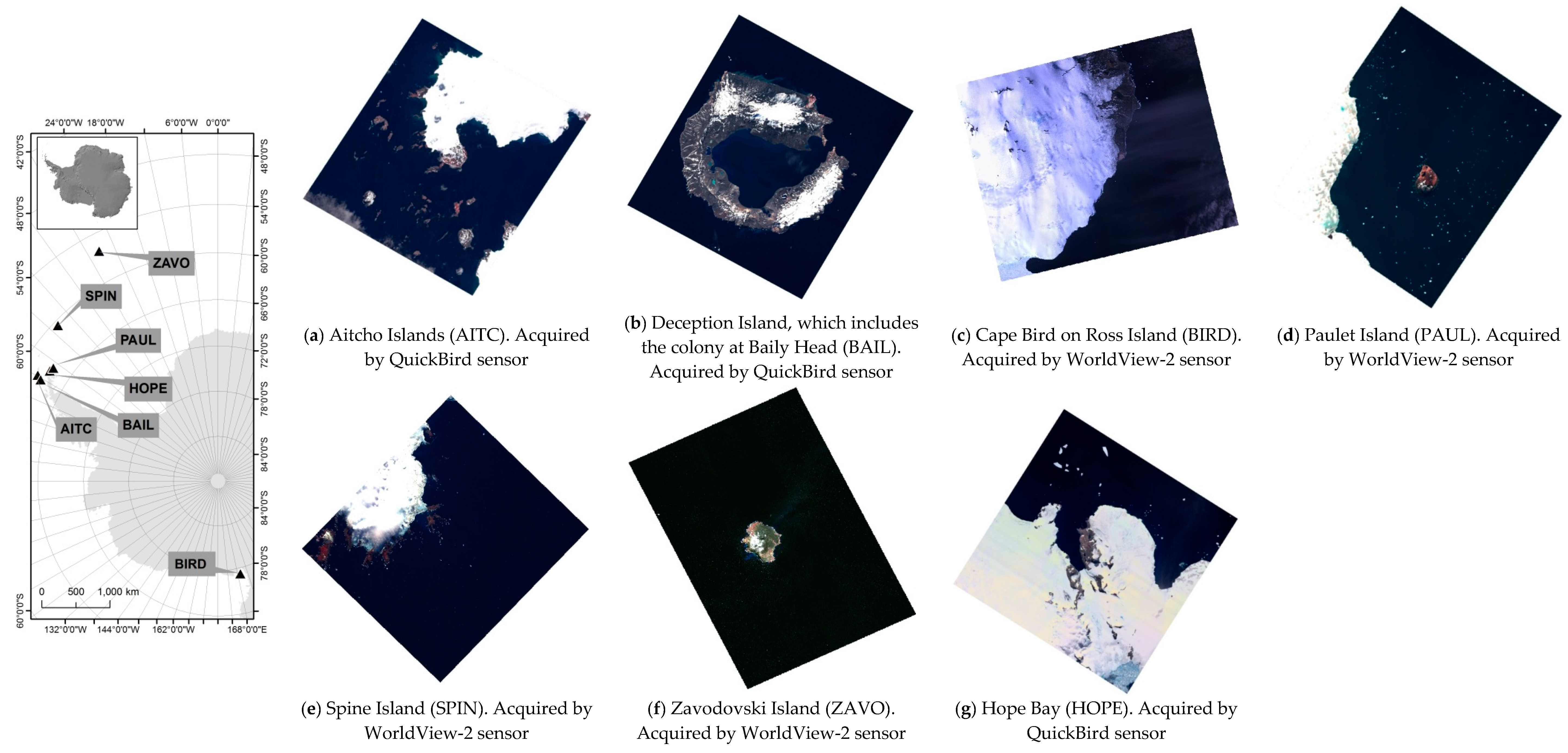
2.1. Study Area and Image Data

In this study, we used a set of cloud-free QuickBird-2 and Worldview-2 images (Figure 1) over sites containing either Adélie or chinstrap penguin colonies (

Table 1. Abundance information of candidate sites.

Site	Coordinates (Lat, Lon)	Species	# of Pairs	Source
Barrientos Island in the Aitcho Islands	−62.381, −59.776	Chinstrap	4047	[54]
Baily Head, Deception Island	−62.967, −60.500	Chinstrap	50,408	[55]
Spine Island	−60.594, −46.020	Chinstrap	unknown	[56]
Hope Bay	−63.397, −56.998	Adélie	~100,000	[20]
Paulet Island	−63.581, −55.788	Adélie	~100,000	[20]
Cape Bird	−77.229, 166.413	Adélie	66,679	[57]
Zavodovski Island	56.298, −27.577	Chinstrap	~600,000	[58]
		Macaroni	~90,000

).

Colonies are generally too large to count all at once, so they are divided up by the surveyor(s) into easily distinguished sub-groups. In each sub-group, the number of nests (or chicks, depending on the time of year) are counted three times using a handheld tally counter. Each count is required to be within 5% of each other and if they are not, the process is repeated. The average of the three counts are used to determine to total number of breeding pairs at a given site. The candidate locations have been previously surveyed on the ground and therefore automated classification could be validated against prior experience, photodocumentation, and existing GPS data on colony locations. Both Adélie and chinstrap penguins form tightly packed breeding colonies, which aids in the interpretation of satellite imagery. Gentoo penguins (P. papua) also breed in this area, but their colonies are more difficult to interpret in satellite imagery (even for an experienced interpreter) because they often nest in smaller groupings or at irregular densities that can weaken the guano stain signature. For this reason, while Gentoo penguins breed in the Aitcho Islands, and at other locations that might have been included in our study, we have excluded them from this analysis.

Candidate scenes that have been radiometrically corrected, orthorectified, and spatially registered to the WGS 84 datum and the Stereographic South Pole projection were provided by the Polar Geospatial Center (University Minnesota). The QuickBird-2 sensor has a ground sampling distance (GSD) of 0.61 cm for the PAN and 2.44 m for MS bands at nadir with 11-bit radiometric resolution. The Worldview-2 hyperspatial sensor records the PAN and the 8 MS bands with a GSD of 0.46 m and 1.84 m at nadir, respectively.

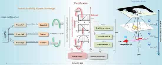
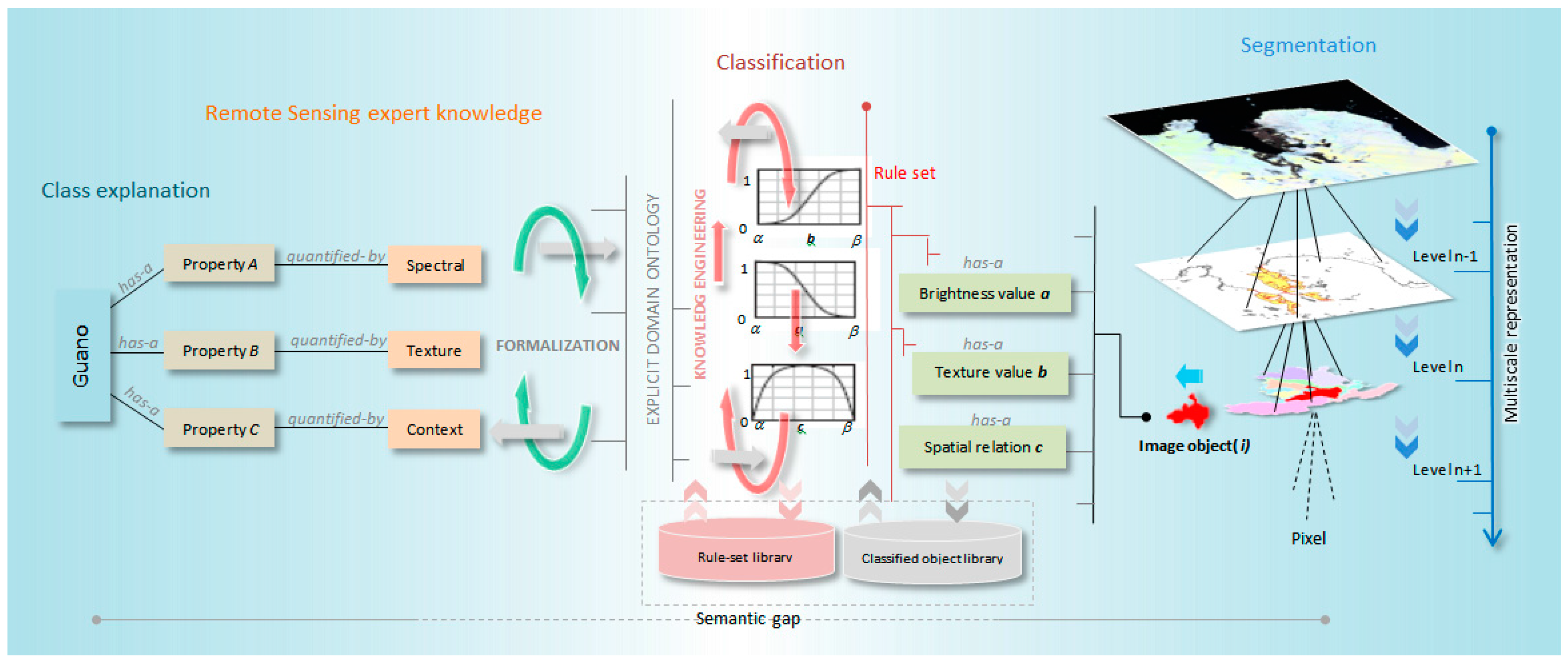
2.2. Conceptual Framewok

While VHSR sensors enable the detection of a single seal (or, under some circumstances, a penguin) hauled out on pack ice, it remains very difficult to intelligently transform very high resolution image pixels to predefined semantic labels. Automated processes for interpreting VHSR imagery are increasingly critical because recent policy easements allow the release of 0.31 m resolution satellite images (e.g., WorldView 3) for civilian use, and the number of commercial satellites supplying EO imagery continues to grow. While there are some developments in fully-automated VHSR image interpretation, the intriguing question of “how to meaningfully link RS quantifications and user defined class labels” remains largely unanswered and voices the argument of considering this issue as a technological challenge rather a broader knowledge management problem [59] in VHRS image processing. To address the “big data” challenge in EO of Antarctic wildlife, we propose a conceptual outline (Figure 2), which resonates with the framework of [59], for automated segmentation and classification of guano in VHSR imagery. In this framework, scene complexity is reduced through multi-scale segmentation, which incorporates multisource RS/GIS/thematic data and creates a hierarchical object structure based on the premise that real world features are found in an image at different scales of analysis [36]. Image object candidates extracted at different scales are adaptively streamed into semantic categories through knowledge-based classification (KBC), which interfaces low-level image object features and expert knowledge by means of fuzzy membership functions. The classified image objects can then be integrated into ecological models; for example, areas of guano staining can be used to estimate the abundance of breeding penguins [22].

In a cyclic manner, classified image objects and model outputs are further integrated into the segmentation and rule-set tuning process. Operator- and scene-dependency of rulesets can impair the repeatability and transferability of KBC workflows across scenes and sensors for the same land cover of interest. We propose to organize rulesets into target- and sensor-specific libraries [59,60] and systematically store a set of classified image objects as “bag-of-image-objects” (BIO) for refining and adapting KBC workflows.

It is important to emphasize that our approach is not a fully-developed system architecture but instead represents a road map for an “image-to-assessment pipeline” that links integral components like class explanation, remote sensing expert knowledge, domain ontology [61,62], multiscale image content modeling, and ecological model integration. This work is crucial to decision support software that links image interpretation with statistical models of occupancy (presence and absence of populations) and abundance and, at a subsequent step, model exploration applications that allow stakeholders to perform geographic searches for populations, aggregate abundance across areas of interest (e.g., proposed Marine Protected Areas), and visualize predicted dynamics for future years. In this exploratory study, we develop those elements critical to the image interpretation components of this pipeline, specifically image segmentation, object-based classification, and ruleset transferability.

2.3. Image Segmentation

When thinking beyond perfect image object candidates (i.e., an ideal correspondence between an image object and a real-world entity), two failure modes expected in segmentation are over-segmentation and under-segmentation [37,40,63]. The former is generally acceptable, although it could be problematic if the geometric properties of image object candidates are used in the classification step. The latter is highly unfavorable because the resulting segments represent a mixture of elements that cannot be assigned a single target class [37,47]. Thus, better classification accuracy hinges on optimal segmentation, in which the average size of image objects is similar to that of the targeted real-world objects [40,64,65,66,67].

Image segmentation is inherently a time- and processor-intense process. The processing time exponentially rises with respect to the scene size, spatial resolution, and the size of image segments. We employed two algorithms to make the segmentation process more efficient, a multi-threshold segmentation (MTS) algorithm and a multiresolution segmentation (MRS) algorithm within the eCognition Developer 9.0 (Trimble, Raunheim, Germany) software package. The former is a simple and less time-intense algorithm, which splits the image object domain and classifies resulting image objects based on a defined pixel value threshold. In contrast, the latter is a complex and time-intense algorithm, which partitions the image scene based on both spectral and spatial characteristics, providing an approximate delineation to real-world entities. In the initial passes of segmentation, we employed the MTS algorithm in a self-adaptive manner for regionalizing the entire scene into manageable homogenous segments. The MRS algorithm was then tasked for targeted segments for generating progressively smaller image objects in a multiscale architecture.

2.3.1. Multi-Threshold Segmentation Algorithm

The MTS algorithm uses a combination of histogram-based methods and the homogeneity measurement of multiresolution segmentation to calculate a threshold dividing the selected set of pixels into two subsets whereby the heterogeneity is increased to a maximum [68]. This algorithm splits the image object domain and classifies resulting image objects based on a defined pixel value threshold. The user can define the pixel value threshold or it can operate in self-adaptive manner when coupled with the automatic threshold (ATA) algorithm in eCognition Developer [69]. The ATA algorithm initially calculates the threshold for the entire scene, which is then saved as a scene variable, and makes it available for the MTS algorithms for segmentation. Subsequently, if another pass of segmentation is needed, the ATA algorithm calculates the thresholds for image objects and saves them as object variables for the next iteration of the MTS algorithm.

2.3.2. Multiresolution Segmentation Algorithm

Of the many segmentation algorithms available, multiresolution segmentation (MRS, see [69]) is the most successful segmentation algorithm capable of producing meaningful image objects in many remote sensing application domains [41], though it is relatively complex and image- and user-dependent [37,51]. The MRS algorithm uses the Fractal Net Evolution Approach (FNEA), which iteratively merges pixels based on homogeneity criteria driven by three parameters: scale, shape, and compactness [39,46,47]. The scale parameter is considered the most important, as it controls the relative size of the image objects and has a direct impact on the subsequent classification steps [64,66,70].

2.3.3. Segmentation Quality Evaluation

As discussed previously, optimal segmentation maximizes the accuracy of the classification results. Over-segmentation is acceptable but leads to plurality of solutions while under-segmentation is unfavorable and produces mixed classified objects that defy classification altogether. In this study, we used a supervised metric, namely the Euclidean Distance 2 (ED2), to estimate the quality of segmentation results. This metric optimizes two parameters in Euclidian space: potential-segmentation error (PSE) and the number-of-segmentation ratio (NSR). The PSE gauges the geometrical congruency between reference objects and image segments (image object candidates) while the NSR measures the arithmetic correspondence (i.e., one-to-one, one-to-many, or many-to-one) between the reference and image object candidates. The highest segmentation quality is reported when the calculated ED2 metric value is close to zero. We refer the reader to [46] for further detail on the mathematical formulation of PSE and NSR. In order to generate a reference data set for quality evaluation, we tasked an expert to manually digitize guano stains.

2.4. Quantifying the Transferability of GEOBIA Rulesets

While GEOBIA provides rich opportunities for expert (predefined) knowledge integration for the classification process, it also makes the classification more vulnerable to operator-/scene-/sensor-/target-dependency, which in turn hampers the repeatability and transferability of rules. Building a well-defined ruleset is a time-, labor-, and knowledge-intense task. Assuming that the segmentation process is optimal, robustness of GEOBIA rulesets rely heavily on the design goals of the ruleset describing the target classes of interest (e.g., class description) and their respective properties (e.g., low-level image object features) (see Figure 2).

Table 2. Image object properties and corresponding spectral bands.

Property	Spectral Bands Used
	QuickBird	WorldView-2
Mean brightness	all bands	all bands
Ratio red	relative brightness of the red band against the mean brightness	relative brightness of the red band against the mean brightness
Normalized difference vegetation index (NDVI)	red, NIR	red, NIR1
Normalized difference water index (NDWI)	red, NIR	red, NIR1
Red/Green ratio	red, green	red, green
Gray level co-occurrence matrix (GLCM) dissimilarity	PAN	PAN
Distance to coastline	-	-
Border contrast	PAN	PAN
Gray level co-occurrence matrix (GLCM) contrast	PAN	PAN

lists important spectral, spatial, and textural properties, which we elected for developing the original ruleset.

Use of fuzzy rules (which can take membership values between 0 and 1) is much favored in object-based classification over crisp rules (which can take membership values constrained to two logical values “true” (=1) and “false” (=0)) because the “fuzzification” of expert-steered thresholds improves transferability. In the case of GEOBIA, the classes of interest can be realized as a fuzzy set of image objects where a membership function(s) defines the degree of membership (μ $\in$ [0, 1], μ = 0 means no membership to the class of interest, μ = 1 means the conditions for being a member of the class of interest is completely satisfied) of each image object to the class of interest with respect to a certain property. A fuzzy function describing a property p can be defined using: α (lower border of p), β (upper border of p), a (mean of membership function), and v (range of membership function).

In this study, we employed the framework proposed by [71] for quantifying the robustness of fuzzy rulesets. While briefly explaining the conceptual basis and implementation of the robustness measure, we encourage the reader to refer [71] for further details.

A ruleset is considered to be more robust if it is capable of managing the variability of the target classes detected in different images given that the images are comparable and the segmentation results are optimal. [71] identified three types (C, O, F) of changes that a reference rule set (R_r) is exposed to during adaptation and used them to quantify the total deviation (d) of the adapted ruleset (R_a).

Type C: Adding, removing, or deactivating a class.

Type O: Change of the fuzzy-logic connection of membership functions.

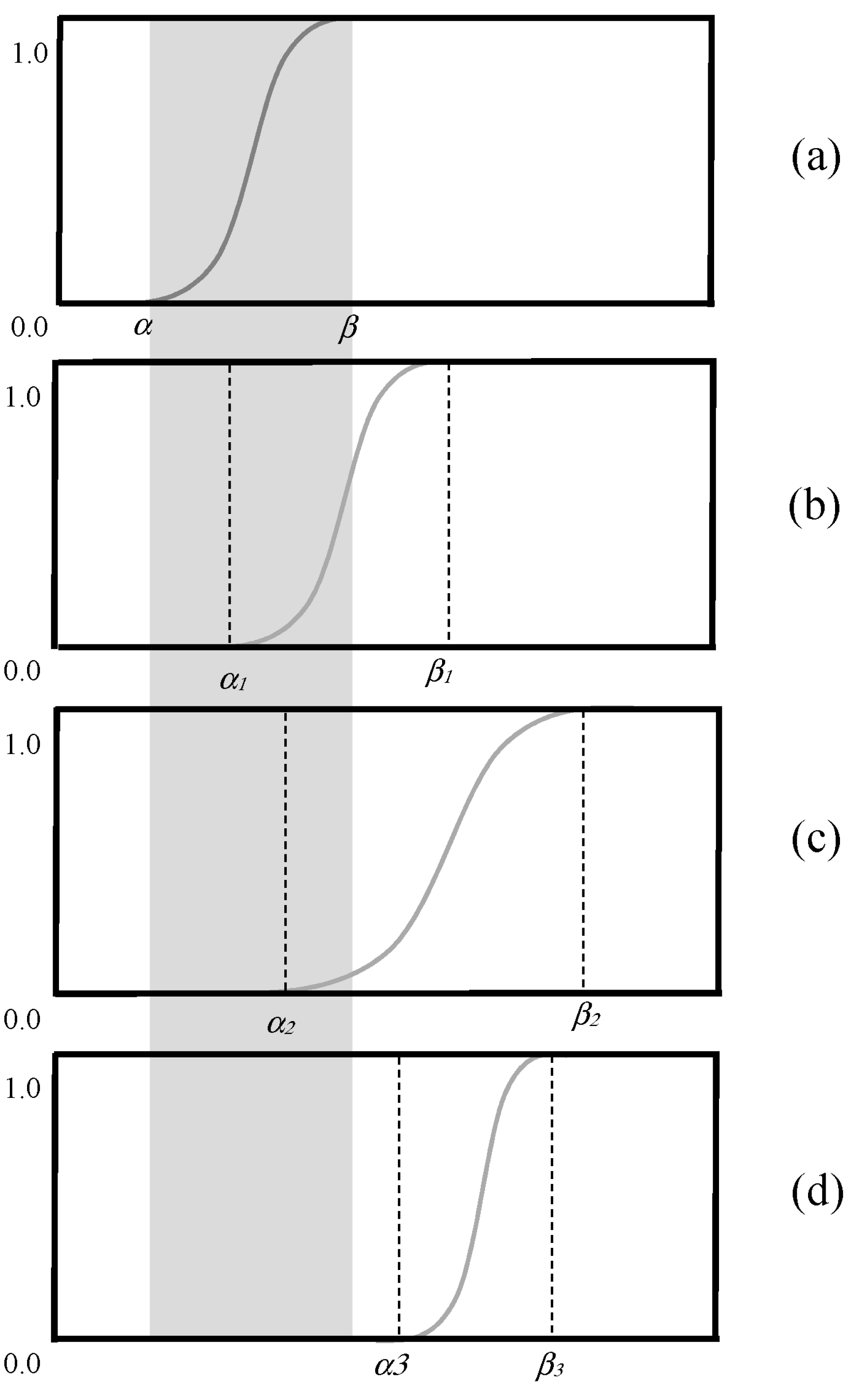
Type F: Inclusion or exclusion (Type F^a) and changing the range of fuzzy membership functions (Type F^b).

The total deviation (d) occurring when adapting R_r to R_a is given by summation of individual changes of Types C, O, and F;

$$d={\displaystyle \sum }_{i=1}^c{\mathrm{C}}_i+{\displaystyle \sum }_{i=1}^{\mathrm{o}}{\mathrm{O}}_i+{\displaystyle \sum }_{i=1}^{f_a}{\mathrm{F}}_i^a+{\displaystyle \sum }_{i=1}^{f_b}\delta F_i^b$$

(1)

$$\delta F = \delta a+\delta \nu$$

(2)

Figure 3 exhibits the possible changes of a membership function, which is subjected to adaptation under Type F^b. Let R_r be the master ruleset [72] developed based on the reference image (I_r) and R_a be the adapted version on R_r over a candidate image I (I_a). The robustness (r_r) of the master ruleset can be quantified by coupling with a quality parameter q (q_a and q_r denotes the classification accuracy of image I_a and I_r, respectively) and total deviations associated with R_a (d_a).

$$r_r=\frac{\raisebox{1ex}{$q_a$}\!\left/ \!\raisebox{-1ex}{$q_r$}\right.}{d_a+1}$$

(3)

2.5. Classification Accuracy Assessment

The areas correctly detected (True Positive—TP: correctly extracted pixels), omitted (True Negative—TN: correctly unextracted pixels), or committed (False Positive—FP: incorrectly extracted pixels) were computed by comparison to the manually-extracted guano stains. Based on these areas the Correctness, Completeness, and Quality indices were computed as follows [73,74]:

$$\text{Correctness}= \frac{\text{TP}}{\text{TP}+\text{FP}}$$

(4)

$$\text{Completeness}= \frac{\text{TP}}{\text{TP}+\text{FN}}$$

(5)

$$\text{Quality}= \frac{\text{TP}}{\text{TP}+\text{FP}+\text{TN}}$$

(6)

Correctness is a measure ranging between 0 and 1 that indicates the detection accuracy rate relative to ground truth. It can be interpreted as the converse of commission error. Completeness is also a measure ranging from 0 and 1 that can be interpreted as the converse of omission error. The two metrics are complementary measures and should be interpreted simultaneously. For example, if all scene pixels are classified as TPs, then the Completeness value approaches 1 while the Correctness approaches 0. Quality is a more meaningful metric that normalizes the Completeness and Correctness. The Quality measure can never be higher than either the Completeness or Correctness. The Quality parameter (Equation (6)) is then used as q in Equation (3) to compute the robustness of the master ruleset in each adaptation.

3. Results

3.1. Segmentaion Quality and Classfication Accuracy

Table 3. A site-wise summary of segmentation quality and classification accuracy.

Site	Segmentation Quality			Classification Accuracy
	NSR	PSE	ED2	Correctness		Completeness		Quality
				Reference Ruleset	Adapted Ruleset	Reference Ruleset	Adapted Ruleset	Reference Ruleset	Adapted Ruleset
AITC	1.43	0.10	1.44	44.8	29.3	17.1	52.2	14.1	23.1
BAIL	1.13	0.10	1.14	58.3	79.1	49.9	80.5	36.8	66.4
BIRD	2.73	0.05	2.73	50.8	66.6	51.4	96.6	34.3	65.1
HOPE	0.20	0.22	0.30	70.0		73.60		55.9
PAUL	4.03	0.14	4.03	34.8	66.4	11.6	79.9	9.5	56.9
SPIN	4.40	0.09	4.40	62.1	64.7	20.3	78.2	18.1	54.8
ZAVO	7.53	0.05	7.53	0.0	73.5	0.0	72.0	0.0	57.2

AITC—Aitcho Islands, BAIL—Baily Head, BIRD—Cape Bird, PAUL—Paulet Island, SPIN—Spine Island, and ZAVO—Zavodovski Island, NSR—number-of-segmentation ratio, PSE—potential segmentation error (PSE), ED2—Euclidian Distance 2.

reports the overall segmentation quality and the classification accuracy. The segmentation quality is evaluated using the number-of-segmentation ratio (NSR), potential segmentation error (PSE), and Euclidian Distance 2 (ED2) for the reference image scene (HOPE) and the candidate image scenes. With respect to the NSR metric, segmentation results from HOPE exhibited the highest arithmetic correspondence while ZAVO exhibited the lowest arithmetic correspondence between the reference objects and the image object candidates. Image segments from PAUL, SPIN, and BIRD reported relatively high NRS values. When analyzing PSE values of each site, BIRD and ZAVO reported the highest geometrical congruency between the manually-digitized targets and the image object candidates. In contrast, despite the high arithmetic fit, HOPE reports the worst geometrical agreement. According to the ED2 metric, which gauges the arithmetic- and geometrical-fit simultaneously, HOPE and ZAVO exhibit the lowest and the highest values, respectively, indicating best and worst segmentation quality. Of the other sites, AITC and BAIL showed relatively low ED2 values manifesting mediocre segmentation quality. The classification accuracy is reported for both the master ruleset and the adapted ruleset based on three parameters: Completeness, Correctness, and Quality. It should be noted that for each of the test-bed sites (AITC, BAIL, BIRD, PAUL, SPIN, and ZAVO), the classification accuracy was individually assessed based on the results obtained by applying the reference ruleset and the adapted ruleset. When the reference ruleset is executed without adaptations, in terms of Correctness, SPIN and ZAVO reported the highest (62.1%) and the lowest (0.0%) detection of targets, respectively. However, compared to HOPE, SPIN exhibited inferior results. In the case of the Completeness metric, BIRD and ZAVO showed the best (51.4%) and worst (0.0%) results while PAUL and AITC marked relatively poor metric values. When comparing metric scores of BIRD and HOPE, the latter shows inferior classification accuracy with respect to the Completeness metric. Even though SPIN reported the highest Correctness, it showed relatively low completeness (20.3%). When analyzing scores reported for the Quality (combined metric of correctness and completeness) metric when the reference ruleset is executed without adaptations, BAIL had the highest classification accuracy (36.8%) while ZAVO reported the lowest accuracy (0.0%). Of the others, BIRD exhibited relatively high classification accuracy (34.3%) while PAUL marked notably low accuracy (9.5%). Similar to Correctness and Completeness, HOPE reported superior results for the Quality metric (55.9%) compared to that of all the testbeds. This highlights the site- and scene-dependency of the master ruleset.

When considering classification accuracy with respect to the adapted ruleset, BAIL and AITC had the highest (79.1%) and the lowest (29.3%) correctness, respectively. ZAVO also yielded a high value (73.5%) and BIRD, PAUL, and SPIN marked comparable scores. Of the testbeds, BAIL and ZAVO reported superior results to HOPE (70.0%). Generally speaking, we can deduce that the adaptations of fuzzy rules have improved the correctness of classification. This fact is well highlighted in ZAVO, where the Correctness metric has been improved from 0.0% to 73.5%. In the case of Completeness, BIRD reported the highest score, which exceeds HOPE while AITC reported the lowest value. Of the other testbeds, BAIL, PAUL, SPIN, and ZAVO yielded high metric scores and the former three exceeded HOPE. In terms of overall classification quality, BAIL was classified with the highest accuracy (66.4%) while AITC had the worst accuracy (23.1%). Overall, BAIL, BIRD, PAUL, SPIN, and ZAVO outperform the accuracy of HOPE, which indicates the success of adaptation.

3.2. Ruleset Adaptation

Table 4. Ruleset adaptation from HOPE to AITC.

Class		Image Object Property (Feature/Variable)	Membership Function	Parameters of the Master Ruleset				Parameters of the Adapted Ruleset				Deviations
												Type Fb			Type Fa
				αr	βr	vr	αr	αa	βa	va	aa	δv	δa	δF	Add/Remove/Change
Top level Level I	Snow/Wave crest/Cloud	Brightness		80.0	100.0	20.0	90.0	55.00	65.00	10.00	60.00	1.00	0.5	1.5	-
	Land	Ratio red		0.85	1.00	0.15	0.93	0.70	1.00	0.30	0.85	0.00	0.09	0.09	-
	Water	NDWI		0.40	0.60	0.20	0.50	0.40	0.60	0.20	0.50	0.00	0.00	0.00	-
	Shadows	NDWI		0.15	0.40	0.25	0.28	0.15	0.40	0.25	0.28	0.00	0.00	0.00	-
Base level Level I1	Snow/Wave crest/Cloud	Brightness		55.0	65.0	10.0	60.0	60.00	70.00	10.00	65.00	0.00	0.08	0.08	-
	Water	NDWI		0.30	0.40	0.10	0.35	0.30	0.40	0.10	0.35	0.00	0.00	0.00	-
	Vegetation	NDVI		0.12	0.14	0.02	0.13	0.20	0.25	0.05	0.23	0.06	0.43	0.49	-
	Shadows/small dark objects	NDWI		0.15	0.40	0.25	0.28	0.01	0.25	0.24	0.13	0.04	1.15	1.19	-
	Bare earth/rock	Red/Green ratio		0.70	0.90	0.20	0.80	0.80	0.95	0.15	0.88	0.33	0.09	0.42	-
	Guano	Red/Green ratio		0.95	0.90	0.05	0.98	0.99	1.10	0.01	1.00	4.00	0.98	4.98	-
		GLCM Dissimilarity		3.00	4.00	1.00	3.50	1.75	2.25	0.50	2.00	1.00	0.75	1.75	-
		Distance to coastline (m)		50.00	1500.00	1450.00	725.00	50.00	1500.00	1450.00	725.00	0.00	0.00	0.00	-
		Border contrast		2.50	3.50	1.00	3.00	2.00	3.00	1.00	2.50	0.00	1.00	1.00	-
		GLCM Contrast		10.00	14.00	4.00	12.00	6.00	7.00	1.00	6.50	3.00	0.85	3.85	-

NDWI—Normalized difference water index, NDVI—Normalized difference vegetation index, GLCM—Gray level co-occurrence matrix. For a fuzzy membership function describing property p: α—lower border, β—upper border, v—range, a—mean. Subscripts r and a denote reference ruleset and adapted ruleset, respectively.

,

Table 5. Ruleset adaptation from HOPE to BAIL.

Class		Image Object Property (Feature/Variable)	Membership Function	Parameters of the Master Ruleset				Parameters of the Adapted Ruleset				Deviations
												Type Fb			Type Fa
				αr	βr	vr	αr	αa	βa	va	aa	δv	δa	δF	Add/Remove/Change
Top level Level I	Snow/Wave crest/Cloud	Brightness		80.0	100.0	20.0	90.0	70.0	90.0	20.0	80.0	0.0	0.13	0.13	-
	Land	Ratio red		0.85	1.00	0.15	0.93	0.75	1.00	0.25	0.88	0.04	0.06	0.10	-
	Water	NDWI		0.40	0.60	0.20	0.50	0.50	0.60	0.10	0.55	1.00	0.09	1.09	-
	Shadows	NDWI		0.15	0.40	0.25	0.28	-	-	-	-	-	-	-	inactive
Base level Level I1	Snow/Wave crest/Cloud	Brightness		55.0	65.0	10.0	60.0	55.0	60.0	5.0	58.0	1.00	0.03	1.03	-
	Water	NDWI		0.30	0.40	0.10	0.35	0.50	0.60	0.10	0.55	1.00	0.09	1.09	-
	Vegetation	NDVI		0.12	0.14	0.02	0.13	0.18	0.20	0.02	0.19	0.00	0.32	0.32	-
	Shadows/small dark objects	NDWI		0.15	0.40	0.25	0.28	0.25	0.50	0.25	0.38	0.00	0.26	0.26	-
	Bare earth/rock	Red/Green ratio		0.70	0.90	0.20	0.80	0.70	0.90	0.20	0.80	0.00	0.00	0.00	-
	Guano	Red/Green ratio		0.90	0.95	0.05	0.98	0.95	1.00	0.05	0.98	0.00	0.00	0.00	-
		GLCM Dissimilarity		3.00	4.00	1.00	3.50	2.30	2.50	0.20	2.40	0.50	0.46	0.96	-
		Distance to coastline (m)		50.00	1500.00	1450.00	725.00	25.00	1150.00	1125.00	587.50	0.29	0.23	0.52	-
		Border contrast		2.50	3.50	1.00	3.00	2.00	6.00	4.00	4.00	0.75	0.25	1.00	-
		GLCM Contrast		10.00	14.00	4.00	12.00	6.00	7.00	1.00	6.50	3.00	0.85	3.85	-

NDWI—Normalized difference water index, NDVI—Normalized difference vegetation index, GLCM—Gray level co-occurrence matrix. For a fuzzy membership function describing property p: α—lower border, β—upper border, v—range, a—mean. Subscripts r and a denote reference ruleset and adapted ruleset, respectively.

,

Table 6. Ruleset adaptation from HOPE to BIRD.

Class		Image Object Property (Feature/Variable)	Membership Function	Parameters of the Master Ruleset				Parameters of the Adapted Ruleset				Deviations
												Type Fb			Type Fa
				αr	βr	vr	αr	αa	βa	va	aa	δv	δa	δF	Add/Remove/Change
Top level Level I	Snow/Wave crest/Cloud	Brightness		80.0	100.0	20.0	90.0	60.00	70.00	10.00	65.00	1.00	0.38	1.38	-
	Land	Ratio red		0.85	1.00	0.15	0.93	0.75	1.00	0.25	0.88	0.40	0.06	0.46	-
	Water	NDWI		0.40	0.60	0.20	0.50	0.40	0.60	0.00	0.00	0.00	0.00	0.00	-
	Shadows	NDWI		0.15	0.40	0.25	0.28	0.10	0.30	0.20	0.20	0.25	0.40	0.65	-
Base level Level I1	Snow/Wave crest/Cloud	Brightness		55.0	65.0	10.0	60.0	65.00	75.00	10.00	70.00	0.00	0.14	0.14	-
	Water	NDWI		0.30	0.40	0.10	0.35	0.30	0.40	0.10	0.35	0.00	0.00	0.00	-
	Vegetation	NDVI		0.12	0.14	0.02	0.13	0.12	0.14	0.02	0.13	0.00	0.00	0.00	-
	Shadows/small dark objects	NDWI		0.15	0.40	0.25	0.28	0.15	0.30	0.20	0.20	0.25	0.40	0.65	-
	Bare earth/rock	Red/Green ratio		0.70	0.90	0.20	0.80	0.80	0.95	0.15	0.88	0.33	0.09	0.24	-
	Guano	Red/Green ratio		0.90	0.95	0.05	0.98	0.95	1.00	0.05	0.98	0.00	0.00	0.00	-
		GLCM Dissimilarity		3.00	4.00	1.00	3.50	14.00	16.00	2.00	15.00	0.50	0.77	1.27	-
		Distance to coastline (m)		50.00	1500.00	1450.00	725.00	50.00	1000.0	950.00	525.00	0.53	0.38	0.91	-
		Border contrast		2.50	3.50	1.00	3.00	0.50	2.00	1.50	1.25	0.33	1.40	1.73	-
		GLCM Contrast		10.00	14.00	4.00	12.00	-	-	-	-	-	-	-	inactive

NDWI—Normalized difference water index, NDVI—Normalized difference vegetation index, GLCM—Gray level co-occurrence matrix. For a fuzzy membership function describing property p: α—lower border, β—upper border, v—range, a—mean. Subscripts r and a denote reference ruleset and adapted ruleset, respectively.

,

Table 7. Ruleset adaptation from HOPE to PAUL.

Class		Image Object Property (Feature/Variable)	Membership Function	Parameters of the Master Ruleset				Parameters of the Adapted Ruleset				Deviations
												Type Fb			Type Fa
				αr	βr	vr	αr	αa	βa	va	aa	δv	δa	δF	Add/Remove/Change
Top level Level I	Snow/Wave crest/Cloud	Brightness		80.0	100.0	20.0	90.0	40.00	50.00	10.00	50.00	1.00	0.80	1.80	-
	Land	Ratio red		0.85	1.00	0.15	0.93	0.80	1.00	0.20	0.90	0.25	0.03	0.28	-
	Water	NDWI		0.40	0.60	0.20	0.50	0.50	0.60	0.10	0.55	1.00	0.09	1.09	-
	Shadows	NDWI		0.15	0.40	0.25	0.28	0.10	0.50	0.40	0.30	0.00	0.07	0.07	-
Base level Level I1	Snow/Wave crest/Cloud	Brightness		55.0	65.0	10.0	60.0	85.00	90.00	5.00	88.00	1.00	0.32	1.32	-
	Water	NDWI		0.30	0.40	0.10	0.35	0.50	0.55	0.05	0.53	1.00	0.66	1.66	-
	Vegetation	NDVI		0.12	0.14	0.02	0.13	0.15	0.17	0.02	0.16	0.00	0.19	0.19	-
	Shadows/small dark objects	NDWI		0.15	0.40	0.25	0.28	0.08	0.45	0.37	0.27	0.32	0.04	0.36	-
	Bare earth/rock	Red/Green ratio		0.70	0.90	0.20	0.80	0.75	0.95	0.20	0.85	0.00	0.06	0.06	-
	Guano	Red/Green ratio		0.95	0.90	0.05	0.98	1.00	1.10	0.05	1.05	0.00	0.07	0.07	-
		GLCM Dissimilarity		3.00	4.00	1.00	3.50	1.8	2.00	0.20	1.90	4.00	0.84	4.84	-
		Distance to coastline (m)		50.00	1500.00	1450.00	725.00	50.00	1200.00	1150.00	625.00	0.30	0.16	0.46	-
		Border contrast		2.50	3.50	1.00	3.00	2.00	6.00	4.00	4.00	0.75	0.25	1.00	-
		GLCM Contrast		10.00	14.00	4.00	12.00	6.00	8.00	2.00	7.00	1.00	0.71	1.71	-

NDWI—Normalized difference water index, NDVI—Normalized difference vegetation index, GLCM—Gray level co-occurrence matrix. For a fuzzy membership function describing property p: α—lower border, β—upper border, v—range, a—mean. Subscripts r and a denote reference ruleset and adapted ruleset, respectively.

,

Table 8. Ruleset adaptation from HOPE to SPIN.

Class		Image Object Property (Feature/Variable)	Membership Function	Parameters of the Master Ruleset				Parameters of the Adapted Ruleset				Deviations
												Type Fb			Type Fa
				αr	βr	vr	αr	αa	βa	va	aa	δv	δa	δF	Add/Remove/Change
Top level Level I	Snow/Wave crest/Cloud	Brightness		80.0	100.0	20.0	90.0	30.00	40.00	10.00	35.00	1.00	1.56	2.56	-
	Land	Ratio red		0.85	1.00	0.15	0.93	0.75	0.90	0.15	0.83	0.00	0.12	0.12	-
	Water	NDWI		0.40	0.60	0.20	0.50	0.45	0.55	0.10	0.48	1.00	0.04	1.04	-
	Shadows	NDWI		0.15	0.40	0.25	0.28	0.30	0.45	0.15	0.38	0.67	0.26	0.93	-
Base level Level I1	Snow/Wave crest/Cloud	Brightness		55.0	65.0	10.0	60.0	35.00	45.00	10.00	40.00	0.00	0.50	0.50	-
	Water	NDWI		0.30	0.40	0.10	0.35	0.45	0.50	0.05	0.48	1.00	0.27	1.27	-
	Vegetation	NDVI		0.12	0.14	0.02	0.13	0.12	0.14	0.02	0.13	0.00	0.00	0.00	-
	Shadows/small dark objects	NDWI		0.15	0.40	0.25	0.28	0.10	0.45	0.35	0.28	0.29	0.00	0.00	-
	Bare earth/rock	Red/Green ratio		0.70	0.90	0.20	0.80	0.75	0.95	0.20	0.85	0.00	0.06	0.06	-
	Guano	Red/Green ratio		0.90	0.95	0.05	0.98	0.90	0.95	0.05	0.98	0.00	0.00	0.0	-
		GLCM Dissimilarity		3.00	4.00	1.00	3.50	1.40	1.60	0.20	1.50	0.33	1.33	1.66	-
		Distance to coastline (m)		50.00	1500.00	1450.00	725.00	50.00	1500.00	1450.00	725.00	0.00	0.00	0.00	-
		Border contrast		2.50	3.50	1.00	3.00	-	-	-	-	-	-	-	inactive
		GLCM Contrast		10.00	14.00	4.00	12.00	10.00	14.00	4.00	12.00	0.00	0.00	0.00	-

NDWI—Normalized difference water index, NDVI—Normalized difference vegetation index, GLCM—Gray level co-occurrence matrix. For a fuzzy membership function describing property p: α—lower border, β—upper border, v—range, a—mean. Subscripts r and a denote reference ruleset and adapted ruleset, respectively.

and

Table 9. Ruleset adaptation from HOPE to ZAVO.

Class		Image Object Property (Feature/Variable)	Membership Function	Parameters of the Master Ruleset				Parameters of the Adapted Ruleset				Deviations
												Type Fb			Type Fa
				αr	βr	vr	αr	αa	βa	va	aa	δv	δa	δF	Add/Remove/Change
Top level Level I	Snow/Wave crest/Cloud	Brightness		80.0	100.0	20.0	90.0	125.00	130.00	5.00	127.50	3.00	0.29	3.29	-
	Land	Ratio red		0.85	1.00	0.15	0.93	0.50	1.00	0.50	0.75	0.70	0.24	0.94	-
	Water	NDWI		0.40	0.60	0.20	0.50	0.65	0.70	0.05	0.68	0.60	0.26	0.86	-
	Shadows	NDWI		0.15	0.40	0.25	0.28	0.55	0.65	0.15	0.63	0.67	0.56	1.23	-
Base level Level I1	Snow/Wave crest/Cloud	Brightness		55.0	65.0	10.0	60.0	160	170	10.00	165.00	0.00	0.63	0.63	-
	Water	NDWI		0.30	0.40	0.10	0.35	0.65	0.70	0.05	0.68	1.00	0.49	1.49	-
	Vegetation	NDVI		0.12	0.14	0.02	0.13	0.18	0.20	0.02	0.19	0.00	0.32	0.32	-
	Shadows/small dark objects	NDWI		0.15	0.40	0.25	0.28	0.35	0.50	0.15	0.43	0.67	0.35	1.02	-
	Bare earth/rock	Red/Green ratio		0.70	0.90	0.20	0.80	0.30	0.40	0.10	0.35	1.00	1.29	2.29	-
	Guano	Red/Green ratio		0.95	0.90	0.05	0.98	0.40	0.42	0.02	0.41	1.50	1.39	2.89	-
		GLCM Dissimilarity		3.00	4.00	1.00	3.50	4.30	4.50	0.10	4.35	9.00	0.20	9.20	-
		Distance to coastline (m)		50.00	1500.00	1450.00	725.00	50.00	1500.00	1450.00	725.00	0.00	0.00	0.00	-
		Border contrast		2.50	3.50	1.00	3.00	-	-	-	-	-	-	-	inactive
		GLCM Contrast		10.00	14.00	4.00	12.00	30.00	35.00	5.00	32.50	0.20	0.63	0.83	-

NDWI—Normalized difference water index, NDVI—Normalized difference vegetation index, GLCM—Gray level co-occurrence matrix. For a fuzzy membership function describing property p: α—lower border, β—upper border, v—range, a—mean. Subscripts r and a denote reference ruleset and adapted ruleset, respectively.

document all of the fine-scale adjustments to the fuzzy rules made during the adaptation of the master ruleset from HOPE to each candidate site. We would like to emphasize that the adaptation process only pertains to the fuzzy rules but not to the segmentation process. Parameter settings of the segmentation algorithms (e.g., scale, shape, compactness values of the MRS algorithm) were fine tuned on a trial-and-error basis at each site until an acceptable segmentation quality was met. Because we wanted to elaborate on the concept of “middleware ruleset” [74] in this analysis, we primarily focused on the changes occurring to the most operative fuzzy rules in the master ruleset. From that respect, in addition to the information reported in Table 4, Table 5, Table 6, Table 7, Table 8 and Table 9, there is always potential for having higher or lower levels in the class hierarchy and scene-specific fuzzy rules for the sake of high classification accuracy. Table 4 summarizes the ruleset adaptations pertaining to AITC. Of all rules, 10 membership functions exhibited Type F^b changes while the others remained unchanged. The highest deviation (δF = 4.98) was reported by Red/Green ratio rule under the class Guano. As seen on Table 5, BAIL reported three Type F^b changes and one Type F^a change at Level I while at Level II a majority of classes showed only Type F^b changes. In the case of class Guano, the fuzzy membership function of Red/Green ratio remained intact while all other associated rules exhibited both limit (upper and lower) and range changes in their fuzzy membership functions. Of all fuzzy rules, the GLCM contrast rule marked the highest total deviation (δF) of 3.85. When the master ruleset was adapted to BIRD (Table 6), two membership functions remained unchanged at Level I, three membership functions exhibited no changes at Level II. With respect to the class Guano, the Red/Green ratio rule was intact, the GLCM contrast rule was kept inactive, and the remaining rules had changes in their fuzzy functions. As seen on Table 7, all of PAUL’s fuzzy membership functions at both Level I and II have undergone Type F^b changes. In certain instances, the membership function has shifted while keeping the range (δv) intact. For example, the Red/Green ratio rule of class Guano exhibited a positive shift from 0.90 to 0.95 (lower border) and 0.95 to 1.10 (upper border) while maintaining a zero change in the range (δv). In the case of class Guano, the highest deviation (δF) exhibited by GLCM dissimilarity while the lowest (0.07) was marked by the Red/Green ratio. Adaptation of the master rule set from HOPE to SPIN (Table 8) reported seven Type F^b changes and one Type F^a change. At Level II, five fuzzy membership functions showed no changes (δF = 0); of those, three are associated with the class Guano, in which the border contrast rule was kept silent. Table 9 lists the ruleset adaptations associated with ZAVO. Under the class Guano, the border contrast rule was kept inactive, which contributed to a Type F^a deviation. The distance to coastline rule remained unchanged while other rules contributed to Type F^b changes, of those the GLCM dissimilarity rule marked the highest total deviation (δF = 9.20).

3.3. Site-Wise Summary

Table 10. A site-wise summary of type and total amount of deviation required for adaptation.

Study Site	Type C	Type O	Type Fa	Type Fb	d
AITC	0	0	0	15.4	15.4
BAIL	0	0	1	10.4	11.4
BIRD	0	0	1	7.43	8.43
PAUL	0	0	0	14.9	14.9
SPIN	0	0	1	8.0	9.0
ZAVO	0	0	1	25.0	26.0

AITC—Aitcho Islands, BAIL—Baily Head, BIRD—Cape Bird, PAUL—Paulet Island, SPIN—Spine Island, and ZAVO—Zavodovski Island, d—total deviation.

provides a site-wise summary of the type and the total amount of deviations associated with each study site. None of the sites reported Type C and Type O deviations. BAIL, BIRD, SPIN, and ZAVO exhibited Type F^a changes. All sites reported Type F^b changes, of those, the highest and the lowest marked by ZAVO (25.0) and SPIN (7.43). In terms of total deviations (d), ZAVO (26.0) and BIRD (8.43) emerged as the highest and lowest candidates. Among the others, AITC and PAUL showed relatively large total deviations.

Table 11. Robustness of the master ruleset when adapted from the reference image to the candidate image.

Site	Robustness
	d = 0	d = d
AITC	0.413	0.025
BAIL	1.188	0.095
BIRD	1.165	0.123
PAUL	1.018	0.064
SPIN	0.980	0.098
ZAVO	1.023	0.038

AITC—Aitcho Islands, BAIL—Baily Head, BIRD—Cape Bird, PAUL—Paulet Island, SPIN—Spine Island, and ZAVO—Zavodovski Island, d—total deviation.

summarizes the robustness of the master ruleset when adapted from the reference image to the each of the candidate image. This measure is based on the classification accuracy (quality parameter pertaining to reference ruleset and adapted ruleset in Table 3) and the total deviations in the ruleset (d value in Table 10). Of all candidate sites, BIRD and AITC recorded the highest (0.123) and the lowest (0.025) robustness values, respectively. The remaining sites ranked from the highest robustness to the lowest robustness as: SPIN > BAIL > PAUL > ZAVO.

3.4. Visual Inspection

We have corroborated the quantitative analysis with visual inspections. Figure 4 shows a set of representative zoomed-in areas selected from the reference image scene (HOPE) and the six candidate images scenes. Classification results achieved by tasking the reference ruleset and the adapted ruleset have been draped (shown in red) over the original multispectral images. For visual clarity, white arrows have been drawn on the reference and the candidate image scenes to point some of the exemplar guano stains. When inspecting the classification results of HOPE, it is clear that the reference ruleset has been fine-tuned to successfully discriminate the targets on the reference image scene. When the reference ruleset is tasked without adaptation, ZAVO exhibited a zero detection of guano stains while others showed some sort of detection. Of those, BAIL and BIRD noted relatively high accurate and complete detection of guano patches. A distinct improvement of the classification accuracy can be observed when the reference ruleset is applied after adaptations. A section of the reference ruleset, which was based on the QuickBird image scene from Hope Bay area and programmed in Cognitive Network Language (CNL) is also provided for the sake of understanding the implementation workflow.

4. Discussion

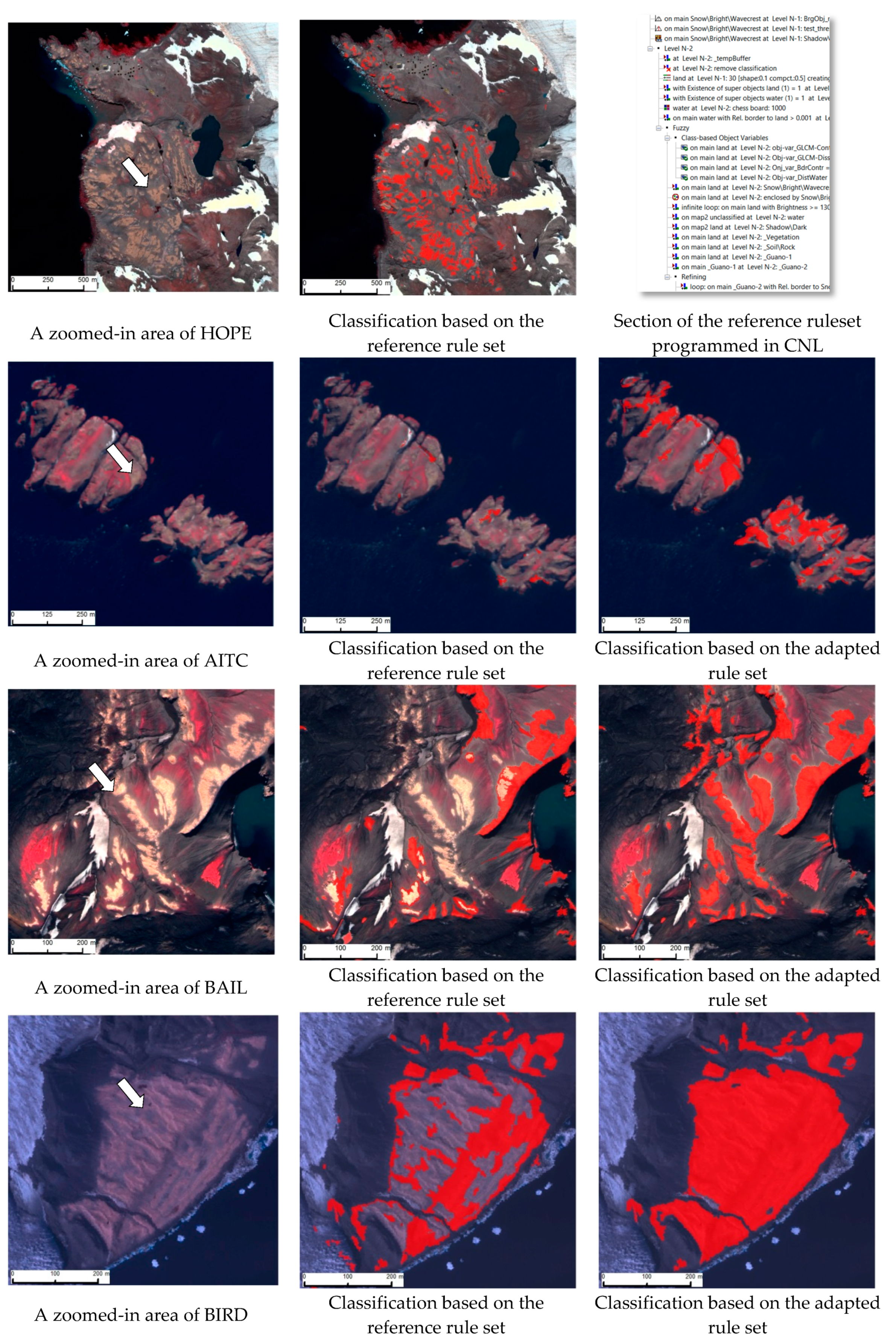
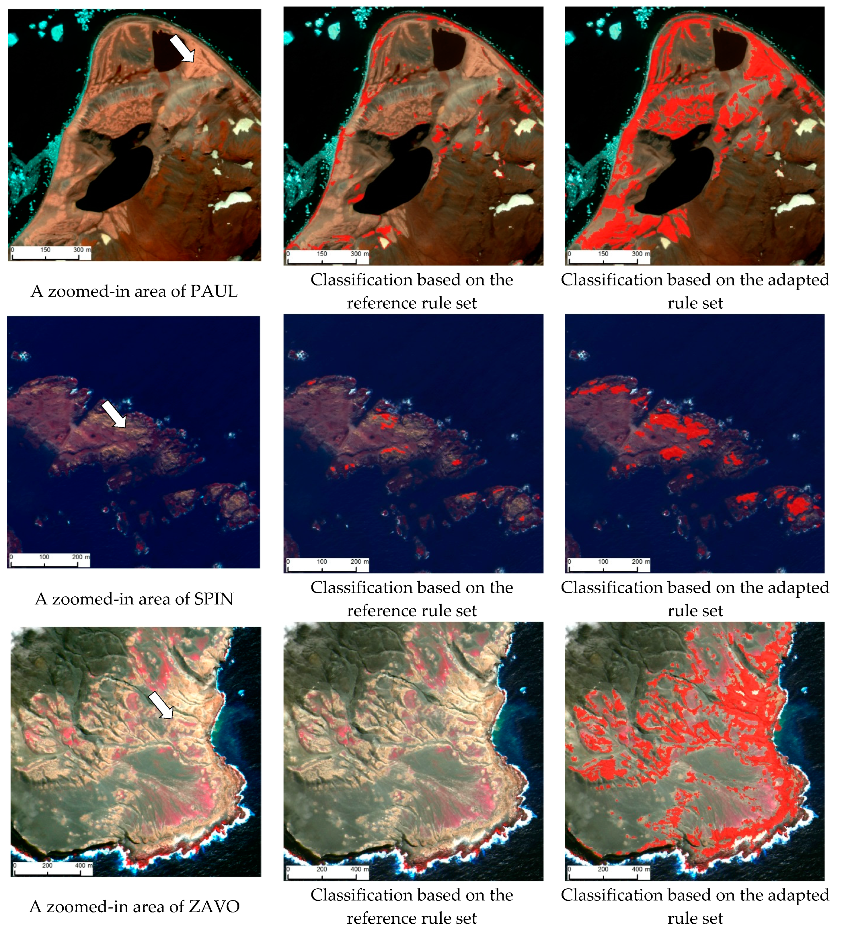
This is the first attempt of which we are aware to use of geographic object-based image analysis paradigm in penguin guano stain detection as an alternative for time- and labor-intensive human-augmented image interpretation. In this exploratory study, we tasked object-based methods to classify chinstrap and Adélie guano stains from very high spatial resolution satellite imagery and closely examined the transferability of knowledge-based GEOBIA rules across different study sites focusing on the same semantic class. A master ruleset was developed based on a QuickBird image scene encompassing the Hope Bay area and it was re-tasked “without adaptation” and “with adaptation” on candidate image scenes (QuickBird and WorldView-2) comprising guano stains from six different study sites. The modular design of our experiment aimed to systematically gauge the segmentation quality, classification accuracy, and the robustness of fuzzy rulesets.

Image segmentation serves as the precursor step in the GEOBIA. Based on the highlighted success rate, in this study, we used eCognition developer’s multiresolution segmentation (MRS) algorithm and complemented it with the multi-threshold segmentation (MTS) algorithm, which can be manipulated in a self-adaptive manner. The underlying idea of coupling MTS and MRS algorithms is to initially reduce the scene complexity at multiscale settings and later feed those “pointer segments” (semantically ill-defined and mixed objects) to the MRS algorithm for more meaningful fine-scale segmentation that creates segments resembling real-world target objects. This hybrid procedure consumes notably less time for scene-wise segmentation than tasking the complex MRS algorithm alone over the entire scene. Segmentation algorithms are inherently scene dependent, which impairs the transferability of a particular segmentation algorithm’s parameter settings (e.g., scale parameter of the MRS algorithm) from one scene to another. Thus, we fine-tuned the segmentation process on a trial-and-error basis at each study site until an acceptable segmentation quality was achieved before tasking either master or adapted rulesets. In general, optimal segmentation results, an equilibrium stage of under- and over-segmentation, are favored for achieving a better classification. From that respect, we purposely employed an empirical segmentation quality measure- Euclidean Distance 2 (ED2), which operates on arithmetic and geometric agreement between reference objects and the image object candidates. Compared to other sites, HOPE reported equally high geometric and arithmetic fit yielding the best overall segmentation quality (lowest ED2). The marked spectral contrast between the guano stains and the dark background materials has led to a better delineation of object boundaries in the segmentation process. In contrast, ZAVO showed the highest ED2 metric value, which was mainly due to the weak arithmetic congruency (high NSR score) at the expense of high geometrical fit. A similar trend can be observed in the remaining study sites as well, for example, BIRD, PAUL, and SPIN. This “one-to-many” relationship between the reference objects and the image object candidates arises primarily due to two reasons: (1) the occurrence of target objects at multiple scales, which impairs the proper isolation of object boundaries at a single scale; (2) when producing reference objects, human interpreters tend to generalize object boundaries [75] based on their experience and semantic meanings of objects than low-level image features like color, texture, or shape. It is interesting to see the fact that study sites with high ED2 scores (poor segmentation quality) have achieved higher classification accuracy than the sites with low ED2 scores. For example, overall classification accuracy (Table 3) of ZAVO has surpassed that of HOPE. By performing a segmentation quality evaluation, we aimed to rule out the possibility that the variations in classification accuracies across candidate study sites attributed not merely because of perturbations in fuzzy rules but because of inferior or superior segmentation.

GEOBIA’s wide adoption in VSHR image based land use land cover (LULC) mapping reflects the fact that object-based workflows are more transferable across image scenes than alternative image analysis methods. However, GEOBIA cannot explicitly link low-level image attributes encoded in image object candidates to high-level user expectations (semantics). While the challenge is universal to VHSR image based LULC mapping in general, within the scope of this study, the intriguing question is “what is the degree of transferability of a master ruleset for guano across scenes and across sites?” Designing a master ruleset based on a certain image scene and targeting a set of target classes is a time-, labor-, and knowledge-intensive process as the operator has to choose the optimal object and scene features and variables to meaningfully link class labels and image object candidates. Thus, in an operations context, reapplication of the master ruleset without adaptations across different scenes would be ideal; however, it is highly unrealistic in most image classification scenarios to achieve acceptable classification accuracy without ruleset modification.

When the master ruleset is reapplied without adaptations (Table 3), the QuickBird scene over BAIL and WorldView-2 scene over BIRD showed relatively high detection of guano stains but still the classification accuracies were inferior to the reference QuickBird scene over HOPE. This is mainly due to the similar spectral, textural, and most importantly neighborhood characteristics (spatially-disjoint patches embedded with dark substrate) of the target class in these three study sites. On the other hand, the WorldView-2 scene over ZAVO showed a zero detection of guano stains when the master ruleset was re-tasked as is. One could argue that this is due to the different sensor characteristics, however; results from BAIL and BIRD challenge that argument. We suspect that notably high reflectance of clouds and wave crests, spectral characteristics of guano, and the hierarchical design (labelling of sub-objects based on super-objects) may have led to an ill detection of guano. From the view point of “ruleset without adaptations”, our analysis reveals that the success rate of the master ruleset’s repeatability is low and unpredictable even in instances where the classification is constrained to a particular semantic class. As seen in Table 3, scene- or site-specific adaptations inevitably enhance the classification accuracy at the expense of operator engagement in re-tuning of fuzzy rules.

When revisiting the fine-scale adjustments associated with the fuzzy rules across all candidate sites (Table 4, Table 5, Table 6, Table 7, Table 8 and Table 9), it is clear that a majority of changes fall onto the Type F^b category, which harbors the changes associated with the underlying fuzzy membership function. In certain instances, for example SPIN and ZAVO, the border contrast rule was left inactive because of the spectral ambiguity between the guano and the surrounding geology. Across all candidate sites, Type F^b deviations have been dominated by the δv component, which elucidates the fact that the shape (range v) of the fuzzy membership function (stretch or shrink) has changed rather than a shift in the mean value (a). This reflects the potential elasticity available to the operator to refine rules. In most cases, our changes to the fuzzy membership functions associated with the class guano are designed to capture the spectral and textural characteristics that distinguish guano stains from the substrate dominating clay minerals like illite and kaolinite [19]. Based on the adapted versions of the master ruleset, study sites like BAIL, BIRD, and ZAVO exhibited superior classification results compared to that of the reference image. Of those, BIRD showed the lowest amount of deviations (d), while ZAVO showed the highest number of total changes in fuzzy membership functions (Table 10). This might be due the fact that HOPE and BIRD share comparable substrate characteristics and contextual arrangement. Except AITC, other candidate sites exhibited either superior or comparable detection of guano stains with respect to the reference image scene. Even the manual delineation of guano stains in AITC was difficult due the existence of guano-like substrate and moss (early stage or dry). This site appeals for inclusion of new rules to discriminate guano rather than simple adaptation of the master ruleset. When considering the robustness of the master ruleset (Table 11) on a site-wide basis and neglecting deviations (d = 0 in Equation (3)), BAIL, BIRD, PAUL, and ZAVO reported highest robustness (r > 1) while AITC reported the lowest. Overall, the mean robustness of all sites is high (0.965), which gives the impression that the master ruleset has been able to produce classification results in all candidate sites almost comparable to the reference study site. When associating Type F^a and Type F^b (d ≠ 0 in Equation (3)) changes to the analysis, site-wise and mean robustness exhibit low values compared to the previous scenario as d penalizes the robustness measure. While accepting the importance of ruleset deviations as a parameter in the robustness measure, we think that Equation (3) does not necessarily include the capacity of the master ruleset to withstand perturbations because the parameter d in the penalization process appears to be asymmetrical. Thus, we realize that the documentation of rule-specific changes and total deviations are of high value in judging the degree of transferability.

The general consensus of the GEOBIA community is to fully exploit all opportunities—spectral, spatial, textural, topological, and contextual features and variables at scene, object, and process levels—available for manipulating image segments in the semantic labelling process. This approach inevitably enhances the classification accuracy; however, it does so at the expense of transferability. We highlight the importance of designing a middleware [76] ruleset, which inherits a certain degree of elasticity rather than a complete master ruleset. From the perspective of knowledge-based classification (KBC), middleware products harbor the optimal set of rules, which combine explicit domain ontology and remote sensing quantifications. In our study, we have purposely confined ourselves to a relatively small number of rules for discriminating focal target classes. These rules are some of the most likely remote sensing quantifications and contextual information that a human interpreter would use in semantic labelling process other than his/her procedural or structured knowledge. There is always potential for introducing higher- and lower-level rules for the middleware products to refine coarse- and fine-scale objects, respectively. Rather than opaquely claiming the success of object-based image analysis in a particular classification effort, a systematic categorization and documentation (e.g., Table 4, Table 5, Table 6, Table 7, Table 8 and Table 9) of individual changes in fuzzy membership functions and a summary of overall changes in the reference ruleset (e.g., Table 10) makes the workflow more transparent and provides rich opportunities to analyze the modification required for each property. This helps identify crucial aspects of the rule set, interpret possible reasons for such deviations, and introduce necessary mitigations. Moreover, this kind of retrospective analysis provides valuable insights on the cost (e.g., time, knowledge, and labor) and benefits (classification accuracy) encoded in the workflow.

We are no longer able to rely on low-level image attributes (e.g., color, texture, and shape) for describing LULC classes but require high-level semantic interpretations of image scenes. Image semantics are context sensitive, which means that semantics are not an intrinsic property captured during the image acquisition process but rather an emergent property of the interactions of human perception and the image content [77,78,79,80]. GEOBIA’s Achilles’ heel—the semantic gap (lack of explicit link)—impedes repeatability, transferability, and interoperability of classification workflows. On the one hand, the rule-based classification reduces the semantic gap. On the other hand, it leads to plurality of solutions and hampers the transferability due to the need for significant operator involvement. For instance, in this study, another level of thematically-rich guano classification based on species (e.g., Adélie, gentoo, chinstrap, and possibly other seabirds) is critical for ecological model integration and will require deviations in the ruleset across image scenes or even possibly an array of new rules. From a conceptual perspective, we recognize GEOBIA’s main challenge as a knowledge management problem and possibly mitigated with fuzzy ontologies [59,74,75,81]. This serves as the key catalyst for our proposed conceptual sketch (Figure 2) for an “image-to-assessment pipeline” that leverages class explanation, remote sensing expert knowledge, domain ontology, multiscale image content modeling, and ecological model integration. We have proposed the concepts of target- and sensor-specific ruleset libraries and a repository of classified image objects as “bag-of-image-objects” (BIO) for refining and adapting classification workflows. Revisiting our findings, we should highlight that the deviations in the master ruleset across sites (also sensors) are not necessarily influenced by the variations in the class guano itself (Adélie vs. chinstrap penguins) but may be attributed to site-/region-specific characteristics such as existence of extensive vegetation. This precludes the use of a master ruleset that operates at the continent-scale but suggests instead an array of ruleset libraries representing regions, habitats, and possibly different sites within the continent. We emphasize the fact that a deep analysis on what factor(s) affected deviation(s) in a specific rule(s) seriously appeals for new components to the current experiment. Such analysis is beyond the scope of this study. Thus, here we provided plausible causes that hamper the transferability. We did not include gentoo penguins in our study even though their colonies also produce a guano stain visible in satellite imagery because their nesting densities are so highly variable that identification of gentoo colonies in imagery can be challenging even at well-mapped sites. For that reason, segmentation and classification of sites with gentoo penguins should be approached with particular caution until gentoo-specific methods can be developed. Future research will need to focus on a deeper understanding of the specific causes controlling the transferability, the engagement of machine learning algorithms, and a well-structured cognitive experiment to understand human visual reasoning in wildlife detection from remote sensing imagery.

5. Conclusions

We used geographic object-based image analysis (GEOBIA) methods to classify guano stains from very high spatial resolution satellite imagery and closely examined the transferability of knowledge-based GEOBIA rules across different study sites focusing on the same semantic class. We find that object-based methods incorporating spectral, textural, spatial, and contextual characteristics from very high spatial resolution imagery are capable of successful detection of guano stains. Reapplication of the master ruleset on candidate scenes without modifications produced inferior classification results, while tasking of adapted rules produced comparable or superior results compared to the reference image at the expense of operator involvement, time, and transferability. Our findings reflect the necessity of employing a systematic experiment to not only gauge the potential of GEOBIA in a certain classification task but also to identify possible shortcomings, especially from an operational perspective. As EO becomes a more routine method of surveying Antarctic wildlife, findings of this exploratory study will serve as baseline information for Antarctic wildlife researchers to identify opportunities and challenges of GEOBIA as a best-available mapping tool in automated wildlife censusing. In future research, we aim to transform the proposed conceptual sketch—”image-to-assessment pipeline”—into an operational architecture.

References

1. Fraser, W.R.; Trivelpiece, W.Z.; Ainley, D.G.; Trivelpiece, S.G. Increases in Antarctic penguin populations: Reduced competition with whales or a loss of sea ice due to environmental warming? Pol. Biol. 1992, 11, 525–531. [Google Scholar] [CrossRef]
2. Clarke, A.; Murphy, E.J.; Meredith, M.P.; King, J.C.; Peck, L.S.; Barnes, D.K.A.; Smith, R.C. Climate change and the marine ecosystem of the western Antarctic Peninsula. Philos. Trans. R. Soc. B Biol. Sci. 2007, 362, 149–166. [Google Scholar] [CrossRef]
3. Ducklow, H.W.; Baker, K.; Martinson, D.G.; Quetin, L.B.; Ross, R.M.; Smith, R.C.; Stammerjohn, S.E.; Vernet, M.; Fraser, W. Marine pelagic ecosystems: The West Antarctic Peninsula. Philos. Trans. R. Soc. B Biol. Sci. 2007, 362, 67–94. [Google Scholar] [CrossRef]
4. Ainley, D.; Ballard, G.; Blight, L.K.; Ackley, S.; Emslie, S.D.; Lescroël, A.; Olmastroni, S.; Townsend, S.; Tynan, C.T.; Wilson, P.; et al. Impacts of cetaceans on the structure of Southern Ocean food webs. Mar. Mammal Sci. 2010, 26, 482–498. [Google Scholar]
5. Smith, R.C.; Ainley, D.; Baker, K.; Domack, E.; Emslie, S.; Fraser, B.; Kennett, J.; Leventer, A.; Mosley-Thompson, E.; Stammerjohn, S.; et al. Marine ecosystem sensitivity to climate change. BioScience 1999, 49, 393–404. [Google Scholar] [CrossRef]
6. Vaughan, D.G.; Marshall, G.J.; Connolley, W.M.; Parkinson, C.; Mulvaney, R.; Hodgson, D.A.; King, J.C.; Pudsey, C.J.; Turner, J. Recent rapid regional climate warming on the Antarctic Peninsula. Clim. Chang. 2003, 60, 243–274. [Google Scholar] [CrossRef]
7. Mayewski, P.A.; Meredith, M.P.; Summerhayes, C.P.; Turner, J.; Worby, A.; Barrett, P.J.; Casassa, G.; Bertler, N.A.N.; Bracegirdle, T.; Naveira Garabato, A.C.; et al. State of the Antarctic and Southern Ocean climate system. Rev. Geophys. 2009, 47, 231–239. [Google Scholar] [CrossRef]
8. Smith, R.C.; Stammerjohn, S.E. Variations of surface air temperature and sea ice extent in the western Antarctic Peninsula (WAP) region. Ann. Glaciol. 2001, 33, 493–500. [Google Scholar] [CrossRef]
9. Stammerjohn, S.E.; Martinson, D.G.; Smith, R.C.; Iannuzzi, R.A. Sea ice in the Western Antarctic Peninsula region: Spatio-temporal variability from ecological and climate change perspectives. Deep Sea Res. Top. Stud. Oceanogr. 2008, 55, 2041–2058. [Google Scholar] [CrossRef]
10. Ainley, D.G.; Ballard, G.; Emslie, S.D.; Fraser, W.R.; Wilson, P.R.; Woehler, E.J.; Croxall, J.P.; Trathan, P.N.; Murphy, E.J. Adélie penguins and environmental change. Science 2003, 300, 429–430. [Google Scholar] [CrossRef] [PubMed]
11. Atkinson, A.; Siegel, V.; Pakhomov, E.; Rothery, P. Long-term decline in krill stock and increase in salps within the Southern Ocean. Nature 2004, 432, 100–103. [Google Scholar] [CrossRef] [PubMed]
12. Montes-Hugo, M.; Doney, S.C.; Ducklow, H.W.; Fraser, W.; Martinson, D.; Stammerjohn, S.E.; Schofield, O. Recent changes in Phytoplankton Communities associated with rapid regional climate change along the western Antarctic Peninsula. Science 2009, 323, 1470–1473. [Google Scholar] [CrossRef] [PubMed]
13. Lynch, H.J.; Naveen, R.; Trathan, P.N.; Fagan, W.F. Spatially integrated assessment reveals widespread changes in penguin populations on the Antarctic Peninsula. Ecology 2012, 93, 1367–1377. [Google Scholar] [CrossRef] [PubMed]
14. Borboroglu, P.G.; Boersma, P.D. Penguins: Natural History and Conservation; University of Washington Press: Seattle, WA, USA, 2003. [Google Scholar]
15. Ainley, D. The Adélie Penguin: Bellwether of Climate Change; Columbia University Press: New York, NY, USA, 2002. [Google Scholar]
16. Boersma, P.D. Penguins as marine sentinels. BioScience 2008, 58, 597–607. [Google Scholar] [CrossRef]
17. Trathan, P.N.; García-Borboroglu, P.; Boersma, D.; Bost, C.-A.; Crawford, R.J.M.; Crossin, G.T.; Cuthbert, R.J.; Dann, P.; Davis, L.S.; de la Puente, S.; et al. Pollution, habitat loss, fishing, and climate change as critical threats to penguins. Conserv. Biol. 2014, 29, 31–41. [Google Scholar] [CrossRef] [PubMed]
18. Trivelpiece, W.Z.; Hinke, J.T.; Miller, A.K.; Reiss, C.S.; Trivelpiece, S.G.; Watters, G.M. Variability in krill biomass links harvesting and climate warming to penguin population changes in Antarctica. Proc. Natl. Acad. Sci. USA 2011, 108, 7625–7628. [Google Scholar] [CrossRef] [PubMed]
19. Fretwell, P.T.; Phillips, R.A.; Brooke, M.D.L.; Fleming, A.H.; McArthur, A. Using the unique spectral signature of guano to identify unknown seabird colonies. Remote Sens. Environ. 2015, 156, 448–456. [Google Scholar] [CrossRef]
20. Lynch, H.J.; LaRue, M.A. First global census of the Adélie Penguin. Auk 2014, 131, 457–466. [Google Scholar] [CrossRef]
21. Lynch, H.J.; Schwaller, M.R. Mapping the abundance and distribution of Adélie Penguins using Landsat-7: First steps towards an integrated multi-sensor pipeline for tracking populations at the continental scale. PLoS ONE 2014, 9. [Google Scholar] [CrossRef] [PubMed]
22. LaRue, M.A.; Lynch, H.J.; Lyver, P.O.B.; Barton, K.; Ainley, D.G.; Pollard, A.; Fraser, W.R.; Ballard, G. A method for estimating colony sizes of Adélie penguins using remote sensing imagery. Pol. Biol. 2014, 37, 507–517. [Google Scholar] [CrossRef]
23. Schwaller, M.R.; Benninghoff, W.S.; Olson, C.E. Prospects for satellite remote sensing of Adelie penguin rookeries. Int. J. Remote Sens. 1984, 5, 849–853. [Google Scholar] [CrossRef]
24. Schwaller, M.R.; Olson, C.E., Jr.; Ma, Z.; Zhu, Z.; Dahmer, P. A remote sensing analysis of Adélie penguin rookeries. Remote Sens. Environ. 1989, 28, 199–206. [Google Scholar] [CrossRef]
25. Chamaille-Jammes, S.; Guinet, C.; Nicoleau, F.; Argentier, M. A method to assess population changes in king penguins: The use of a Geographical Information System to estimate area-population relationships. Pol. Biol. 2000, 23, 545–549. [Google Scholar] [CrossRef]
26. Trathan, P.N. Image analysis of color aerial photography to estimate penguin population size. Wildl. Soc. Bull. 2004, 32, 332–343. [Google Scholar] [CrossRef]
27. Bhikharidas, A.K.; Whitehead, M.D.; Peterson, J.A. Mapping Adélie penguin rookeries in the Vestfold Hills and Rauer Islands, east Antarctica, using SPOT HRV data. Int. J. Remote Sens. 1992, 13, 1577–1583. [Google Scholar] [CrossRef]
28. Barber-Meyer, S.; Kooyman, G.; Ponganis, P. Estimating the relative abundance of emperor penguins at inaccessible colonies using satellite imagery. Pol. Biol. 2007, 30, 1565–1570. [Google Scholar] [CrossRef]
29. Fretwell, P.T.; Trathan, P.N. Penguins from space: Faecal stains reveal the location of emperor penguin colonies. Glob. Ecol. Biogeogr. 2009, 18, 543–552. [Google Scholar] [CrossRef]
30. Schwaller, M.R.; Southwell, C.J.; Emmerson, L.M. Continental-scale mapping of Adélie penguin colonies from Landsat imagery. Remote Sens. Environ. 2013, 139, 353–364. [Google Scholar] [CrossRef]
31. Southwell, C.; Emmerson, L. Large-scale occupancy surveys in East Antarctica discover new Adélie penguin breeding sites and reveal an expanding breeding distribution. Antarct. Sci. 2013, 25, 531–535. [Google Scholar] [CrossRef]
32. Mustafa, O.; Pfeifer, C.; Peter, H.; Kopp, M.; Metzig, R. Pilot Study on Monitoring Climate-Induced Changes in Penguin Colonies in the Antarctic Using Satellite Images; German Ministry of the Federal Environment: Dessau-Roßlau, Germany, 2012. [Google Scholar]
33. Hay, G.J.; Castilla, G.; Wulder, M.A.; Ruiz, J.R. An automated object-based approach for the multiscale image segmentation of forest scenes. Int. J. Appl. Earth Obs. Geoinf. 2005, 7, 339–359. [Google Scholar] [CrossRef]
34. Baatz, M.; Hoffmann, C.; Willhauck, G. Progressing from object-based to object-oriented image analysis. In Object Based Image Analysis; Blaschke, T., Lang, S., Hay, G.J., Eds.; Springer: Heidelberg, Germany; Berlin, Germany; New York, NY, USA, 2008. [Google Scholar]
35. Marçal, A.R.S.; Rodrigues, A.S. A method for multi-spectral image segmentation evaluation based on synthetic images. Comput. Geosci. 2008, 35, 1574–1581. [Google Scholar] [CrossRef]
36. Blaschke, T. Object based image analysis for remote sensing. ISPRS J. Photogramm. Remote Sens. 2010, 65, 2–16. [Google Scholar] [CrossRef]
37. Marpu, P.R.; Neubert, M.; Herold, H.; Niemeyer, I. Enhanced evaluation of image segmentation results. J. Spat. Sci. 2010, 55, 55–68. [Google Scholar] [CrossRef]
38. Jyothi, B.N.; Babu, G.R.; Murali Krishna, L.V. Object oriented and multi-scale image analysis: Strengths, weaknesses, opportunities and threats—A review. J. Comput. Sci. 2008, 4, 706–712. [Google Scholar] [CrossRef]
39. Smith, G.M.; Morton, R.D. Real world objects in GEOBIA through the exploitation of existing digital cartography and image segmentation. Photogramm. Eng. Remote Sens. 2010, 76, 163–171. [Google Scholar] [CrossRef]
40. Kim, M.; Warner, T.A.; Madden, M.; Atkinson, D.S. Multi-scale GEOBIA with very high spatial resolution digital aerial imagery: Scale, texture and image objects. Int. J. Remote Sens. 2011, 32, 2825–2850. [Google Scholar] [CrossRef]
41. Witharana, C.; Civco, D.L. Optimizing multi-resolution segmentation scale using empirical methods: Exploring the sensitivity of the supervised discrepancy measure Euclidean distance 2 (ED2). ISPRS J. Photogramm. Remote Sens. 2014, 87, 108–121. [Google Scholar] [CrossRef]
42. Lang, S.; Albrecht, F.; Kienberger, S.; Tiede, D. Object validity for operational tasks in a policy context. J. Spat. Sci. 2008, 55, 9–22. [Google Scholar] [CrossRef]
43. Hagenlocher, M.; Lang, S.; Tiede, D. Integrated assessment of the environmental impact of an IDP camp in Sudan based on very high resolution multi-temporal satellite imagery. Remote Sens. Environ. 2012, 126, 27–38. [Google Scholar] [CrossRef]
44. Lang, S. Object-based image analysis for remote sensing applications: Modeling reality—Dealing with complexity. In Object-Based Image Analysis; Blaschke, T., Lang, S., Geoffrey, H., Eds.; Springer: Heidelberg, Germany; Berlin, Germany; New York, NY, USA, 2008. [Google Scholar]
45. Dey, V.; Zhang, Y.; Zhong, M. A review on image segmentation techniques with remote sensing perspective. Int. Arch. Photogramm. Remote Sens. Spat. Inf. Sci. 2010, 38(Part 7A), 31–42. [Google Scholar]
46. Liu, Y.; Bian, L.; Meng, Y.; Wang, H.; Zhang, S.; Yang, Y.; Shao, X.; Wang, B. Discrepancy measures for selecting optimal combination of parameter values in object-based image analysis. ISPRS J. Photogramm. Remote Sens. 2012, 68, 144–156. [Google Scholar] [CrossRef]
47. Tong, H.; Maxwell, T.; Zhang, Y.; Dey, V. A supervised and fuzzy-based approach to determine optimal multi-resolution image segmentation parameters. Photogramm. Eng. Remote Sens. 2012, 78, 1029–1043. [Google Scholar] [CrossRef]
48. Duro, D.C.; Franklin, S.E.; Duba, M.G. A comparison of pixel-based and object-based image analysis with selected machine learning algorithms for the classification of agricultural landscapes using SPOT-5 HRG imagery. Remote Sens. Environ. 2012, 118, 259–272. [Google Scholar] [CrossRef]
49. Blaschke, T.; Hay, G.J.; Kelly, M.; Lang, S.; Hofmann, P.; Addink, E.; Queiroz Feitosa, R.; van der Meer, F.; van der Werff, H.; van Coillie, F.; et al. Geographic object-based image analysis: Towards a new paradigm. ISPRS J. Photogramm. Remote Sens. 2014, 87, 180–191. [Google Scholar] [CrossRef] [PubMed]
50. Burnett, C.; Blaschke, T. A multi-scale segmentation/object relationship modelling methodology for landscape analysis. Ecol. Model. 2003, 168, 233–249. [Google Scholar] [CrossRef]
51. Hay, G.J.; Blaschke, T.; Marceau, D.J.; Bouchard, A. A comparison of three image-object methods for the multiscale analysis of landscape structure. ISPRS J. Photogramm. Remote Sens. 2003, 57, 327–345. [Google Scholar] [CrossRef]
52. Benz, U.C.; Hofmann, P.; Willhauck, G.; Lingenfelder, I.; Heynen, M. Multi-resolution, object-oriented fuzzy analysis of remote sensing data for GIS-ready information. ISPRS J. Photogramm. Remote Sens. 2004, 58, 239–258. [Google Scholar] [CrossRef]
53. Marçal, A.R.S.; Borges, J.S.; Gomes, J.A.; De Costa, J.F.P. Land cover update by supervised classification of segmented ASTER images. Int. J. Remote Sens. 2005, 26, 1347–1362. [Google Scholar] [CrossRef]
54. Lynch, H.; Naveen, R.; Casanovas, P.V. Antarctic site inventory breeding bird survey data 1994/95–2012/13. Ecology 2013. [Google Scholar] [CrossRef]
55. Naveen, R.; Lynch, H.J.; Forrest, S.; Mueller, T.; Polito, M. First direct, site-wide penguin survey at Deception Island, Antarctica suggests significant declines in breeding chinstrap penguins. Pol. Biol. 2012, 35, 1879–1888. [Google Scholar] [CrossRef]
56. Naveen, R.; Lynch, H.J. Antarctic Peninsula Compendium, 3rd ed.; Environmental Protection Agency: Washington, DC, USA, 2011. [Google Scholar]
57. Landcare Research. Available online: http://www.landcareresearch.co.nz/resources/data/adelie-census-data/surveyed-colonies (accessed on 2 October 2013).
58. Lynch, H.J.; White, R.; Naveen, R.; Black, A.; Meixler, M.S.; Fagan, W.F. In stark contrast to widespread declines along the Scotia Arc, a survey of the South Sandwich Islands finds a robust seabird community. Pol. Biol. 2016. [Google Scholar] [CrossRef]
59. Arvor, D.; Durieux, L.; Andrãs, S.; Laporte, M. Advances in geographic object-based image analysis with ontologies: A review of main contributions and limitations from a remote sensing perspective. ISPRS J. Photogramm. Remote Sens. 2013, 82, 125–137. [Google Scholar] [CrossRef]
60. Strasser, T.; Lang, S.; Riedler, B.; Pernkopf, L.; Paccagnel, K. Multiscale object feature library for habitat quality monitoring in riparian forests. IEEE Geosci. Remote Sens. Lett. 2014, 11, 559–563. [Google Scholar] [CrossRef]
61. Bannour, H.; Hudelot, C. Towards ontologies for image interpretation and annotation. In Proceedings of the IEEE 9th International Workshop on Content-Based Multimedia Indexing (CBMI), Madrid, Spain, 13–15 June 2011; pp. 211–216.
62. Kohli, D.; Warwadekar, P.; Kerle, N.; Sliuzas, R.; Stein, A. Transferability of object-oriented image analysis methods for slum identification. Remote Sens. 2013, 5, 4209–4228. [Google Scholar] [CrossRef]
63. Clinton, N.; Holt, A.; Scarborough, J.; Yan, L.; Gong, P. Accuracy assessment measures for object-based image segmentation goodness. Photogramm. Eng. Remote Sens. 2010, 76, 289–299. [Google Scholar] [CrossRef]
64. Dorren, L.K.A.; Maier, B.; Seijmonsbergen, A.C. Improved Landsat-based forest mapping in steep mountainous terrain using object-based classification. For. Ecol. Manag. 2003, 183, 31–46. [Google Scholar] [CrossRef]
65. Addink, E.A.; De Jong, S.M.; Pebesma, E.J. The importance of scale in object-based mapping of vegetation parameters with hyperspectral imagery. Photogramm. Eng. Remote Sens. 2007, 72, 905–912. [Google Scholar] [CrossRef]
66. Smith, A. Image segmentation scale parameter optimization and land cover classification using the Random Forest algorithm. J. Spat. Sci. 2010, 55, 69–79. [Google Scholar] [CrossRef]
67. Myint, S.W.; Gober, P.; Brazel, A.; Grossman-Clarke, S.; Weng, Q. Per-pixel vs. object-based classification of urban land cover extraction using high spatial resolution imagery. Remote Sens. Environ. 2011, 115, 1145–1161. [Google Scholar] [CrossRef]
68. Trimble Germany GmbH. eCognition Developer 8.7.2 Reference Book; Trimble Germany GmbH: Munich, Germany, 2014. [Google Scholar]
69. Baatz, M.; Schäpe, M. Multiresolution segmentation—An optimization approach for high quality multi-scale image segmentation. In Angewandte Geographische Informations-Verarbeitung XII; Strobl, J., Blaschke, T., Griesebner, G., Eds.; Wichmann Verlag: Karlsruhe, Germany, 2000; pp. 12–23. [Google Scholar]
70. Belgiu, M.; Drgut, L.; Strobl, J. Quantitative evaluation of variations in rule-based classifications of land cover in urban neighbourhoods using WorldView-2 imagery. ISPRS J. Photogramm. Remote Sens. 2014, 87, 205–215. [Google Scholar] [CrossRef] [PubMed]
71. Hofmann, P.; Blaschke, T.; Strobl, J. Quantifying the robustness of fuzzy rule sets in object-based image analysis. Int. J. Remote Sen. 2011, 32, 7359–7381. [Google Scholar] [CrossRef]
72. Tiede, D.; Lang, S.; Hölbling, D.; Füreder, P. Transferability of OBIA rulesets for IDP camp analysis in Darfur. In Proceedings of the GEOBIA Geographic Object-Based Image Analysis, Ghent, Belgium, 29 June–2 July 2010.
73. Agouris, P.; Doucette, P.; Stefanidis, A. Automation and digital photogrammetric workstations. In Manual of Photogrammetry; McGlone, C., Mikhail, E., Bethel, J., Eds.; American Society for Photogrammetry and Remote Sensing: Bethesda, MD, USA, 2004; pp. 949–981. [Google Scholar]
74. Argyridis, A.; Argialas, D.P. A fuzzy spatial reasoner for multi-scale GEOBIA ontologies. Photogramm. Eng. Remote Sens. 2015, 81, 491–498. [Google Scholar] [CrossRef]
75. Albrecht, F.; Lang, S.; Hölbling, D. Spatial accuracy assessment of object boundaries for object-based image analysis. Int. Arch. Photogramm. Remote Sens. Spat. Inf. Sci. 2010, XXXVIII-4/C7, 6–10. [Google Scholar]
76. Belgiu, M.; Lampoltshammer, T.J.; Hofer, B. An extension of an ontology-based land cover designation approach for fuzzy rules. In Proceedings of the GI_Forum, Salzburg, Austria, 2–5 July 2013. [CrossRef]
77. Zhao, L.; Tang, P.; Huo, L. A 2-D wavelet decomposition-based bag-of-visual-words model for land-use scene classification. Int. J. Remote Sens. 2015, 35, 2296–2310. [Google Scholar]
78. Gueguen, L.; Datcu, M. A similarity metric for retrieval of compressed objects: Application for mining satellite image time series. IEEE Trans. Knowl. Data Eng. 2008, 20, 562–575. [Google Scholar] [CrossRef]
79. Aksoy, S.; Cinbis, R.G. Image mining using directional spatial constraints. IEEE Geosci. Remote Sens. Lett. 2010, 7, 33–37. [Google Scholar] [CrossRef] [Green Version]
80. Quartulli, M.; Olaizola, I.G. A review of EO image information mining. ISPRS J. Photogramm. Remote Sens. 2013, 75, 11–28. [Google Scholar] [CrossRef]
81. Kohli, D.; Sliuzas, R.; Kerle, N.; Stein, A. An ontology of slums for image-based classification. Comput. Environ. Urban Syst. 2012, 36, 154–163. [Google Scholar] [CrossRef]
Figure 1. Geographical setting of study sites and candidates image scenes: (a) Aitcho Islands (b) Deception Island; (c) Cape Bird on Ross Island (d) Paulet Island; (e) Spine Island; (f) Zavodovski Island; and (g) Hope Bay. Imagery copyright DigitalGlobe, Inc., Westminster, CO, USA.
Remotesensing 08 00375 g001
Figure 2. Object-based penguin guano detection from VHSR images.
Remotesensing 08 00375 g002
Figure 3. Possible changes of membership function during adaptation. (a) initial fuzzy function; (b) adapted: upper and lower border shifted but range fixed; (c) adapted: upper and lower border shifted and range stretched; (d) upper and lower border shifted and the range reduced.
Remotesensing 08 00375 g003
Figure 4. Zoomed-in areas showing: the original image (left); classification based on the reference ruleset (middle); and classification based on the adapted ruleset (right), from the reference study site and the candidate sites. A section of the reference ruleset programmed in Cognitive Network Language (CNL) is also provided at top right. Classified guano is shown in red. Imagery copyright DigitalGlobe, Inc.
Remotesensing 08 00375 g004aRemotesensing 08 00375 g004b