Article

Using Different Regression Methods to Estimate Leaf Nitrogen Content in Rice by Fusing Hyperspectral LiDAR Data and Laser-Induced Chlorophyll Fluorescence Data

1
School of Physics and Technology, Wuhan University, Wuhan 430072, China
2
State Key Laboratory of Information Engineering in Surveying, Mapping and Remote Sensing, Wuhan University, Wuhan 430079, China
3
Collaborative Innovation Center of Geospatial Technology, Wuhan 430079, China
4
School of Resource and Environmental Sciences, Wuhan University, Wuhan 430072, China
*
Authors to whom correspondence should be addressed.
Submission received: 23 February 2016 / Revised: 3 June 2016 / Accepted: 14 June 2016 / Published: 22 June 2016

Abstract

:
Nitrogen is an essential nutrient element in crop photosynthesis and yield improvement. Thus, it is urgent and important to accurately estimate the leaf nitrogen contents (LNC) of crops for precision nitrogen management. Based on the correlation between LNC and reflectance spectra, the hyperspectral LiDAR (HSL) system can determine three-dimensional structural parameters and biochemical changes of crops. Thereby, HSL technology has been widely used to monitor the LNC of crops at leaf and canopy levels. In addition, the laser-induced fluorescence (LIF) of chlorophyll, related to the histological structure and physiological conditions of green plants, can also be utilized to detect nutrient stress in crops. In this study, four regression algorithms, support vector machines (SVMs), partial least squares (PLS) and two artificial neural networks (ANNs), back propagation NNs (BP-NNs) and radial basic function NNs (RBF-NNs), were selected to estimate rice LNC in booting and heading stages based on reflectance and LIF spectra. These four regression algorithms were used for 36 input variables, including the reflectance spectral variables on 32 wavelengths and four peaks of the LIF spectra. A feature weight algorithm was proposed to select different band combinations for the LNC retrieval models. The determination coefficient (R2) and the root mean square error (RMSE) of the retrieval models were utilized to compare their abilities of estimating the rice LNC. The experimental results demonstrate that (I) these four regression methods are useful for estimating rice LNC in the order of RBF-NNs > SVMs > BP-NNs > PLS; (II) The LIF data in two forms, including peaks and indices, display potential in rice LNC retrieval, especially when using the PLS regression (PLSR) model for the relationship of rice LNC with spectral variables. The feature weighting algorithm is an effective and necessary method to determine appropriate band combinations for rice LNC estimation.

Graphical Abstract

1. Introduction

Nitrogen is a crucial nutrient element for plant photosynthesis and it plays a key role in crop yield improvement [1]. The leaf biochemical contents of crops, especially the leaf nitrogen contents (LNC), was an important indicator of the photosynthetic status, which could be estimated to help with illumination of the ecosystem changes over wide scales [2]. Thus, it is urgent and important for precision nitrogen management to accurately estimate the LNC of crops. Kergoat et al. [3] analyzed the relationship between LNC and CO2 flux and concluded that LNC significantly influenced the canopy light use efficiency and canopy photosynthesis rate of vegetation. In recent years, a real-time and nondestructive technique of LNC monitoring of crops has been extensively investigated in the field of remote sensing for precision nitrogen management [4,5,6,7]. These methods can overcome or reduce the issues that passive remote sensing technologies have, such as data redundancy and the effect of irradiation conditions.
Current multispectral remote sensing approaches can monitor the status of crops by analyzing the relationship of canopy nitrogen content and chlorophyll-related spectral responses. However, these passive systems are restricted by many factors, such as weather conditions and monitoring time [8]. To overcome these disadvantages, it is necessary and urgent to develop an active system. Such a system, hyperspectral LiDAR (HSL), can measure both canopy morphologic parameters and biochemical changes using LNC-related reflectance spectra. Applications of HSL to monitor vegetation have been widely conducted both at leaf and canopy levels [5,6]. However, Apostol et al. [9] pointed that the reflectance-based remote sensing methods lack sensitivity for nitrogen detection in early growing stages. Maxwell et al. [10] found that the yield of chlorophyll fluorescence (CF) was quantitatively correlated with the plant photosynthetic system II (PS-II), which was very sensitive to stress from the surrounding environment. During the process of PS-II, plant chloroplasts can harmlessly dissipate residual light energy in the form of heat. Once this heat exceeds the needs of photosynthesis, it will be released by the yield of CF, preventing the oxidative damage of chloroplasts [11]. Coupled with a remote sensing method, the laser-induced fluorescence (LIF) is an attractive and early indicator in detecting the nutrient stress of crops [12,13]. Thus, there is great potential in combining HSL and LIF for crop detection. Although the reflectance spectra are related to the scattering and absorption of light within leaves, the principle of LIF emission is different. Therefore, the challenge of LIF measurement is to separate the apparent reflectance spectra from LIF in leaves [11]. In addition, the magnitude of the time delay between the excitation laser pulse and LIF occurs in nanoseconds; thus, capturing LIF before the deadline is another sufficiently complex challenge [14].
Several researchers focused on relating leaf spectra with several physiological and morphological parameters, such as chlorophyll content [15], LNC [16] and canopy structure [17], which have been proven to be highly correlated with spectral indices. These spectral indices are typically developed in the forms of mathematical formulae. Compared with these spectral indices, LIF indices in blue, green, red and far-red bands can provide significantly more information about the photosynthetic conversion of plants under stress conditions. The study of Lichtenthaler et al. [18] showed that CF indices at 440 nm, 520 nm, 690 nm and 740 nm were highly sensitive to changes in growing and stress conditions. More specifically, under the condition of high light exposure, drought and temperature stress, the fluorescence ratio at blue (440 nm), red (690 nm) and far-red (740 nm) increased significantly [19]. In our study, the LNC of rice was initially estimated based on reflectance spectra and then combined with the LIF spectral data which was regarded as the extra input variable of LNC estimation models.
Several studies have been undertaken to estimate the nitrogen contents of plants using partial least squares regression (PLSR) [20,21,22]. PLSR can be applied to reduce collinear spectral variables to a few non-correlated latent variables (LVs) [23], thereby avoiding overfitting problems. Unlike PLSR, artificial neural networks (ANNs), which are commonly used in remote sensing to predict vegetation parameters and crop yields [24,25], inevitably suffer from overfitting problems. Moreover, the design and implementation of ANNs require complex and time-consuming processes, and their performance can be weakened when low-dimensional datasets are used [21]. Nonetheless, this approach is preferred by many researchers because of its several advantages; for instance, ANNs require neither assumptions concerning the statistical frequency distribution of data nor the measurement scales of the features used in analysis [26,27]. The commonly used models and architectures of ANNs in regression processes are back propagation neural networks (BP-NNs) and radial basic function neural networks (RBF-NNs), which are both employed in this study to estimate the rice LNC. Compared with these methods, the performance of support vector machines (SVMs) seems to be better suited for remote sensing applications than ANNs because of its greater generalizability [28,29]. SVMs reported by several researchers can resolve the problem of overfitting associated with high-dimensional data. ANNs mainly differ from SVMs in terms of the principle of risk minimization (RM) which aims to improve the generalization performance. In using SVMs, an upper bound is minimized by the principle of structural risk minimization (SRM) whereas in using ANNs, traditional empirical risk minimization (ERM) is employed [30]. Recently, SVMs have been applied to estimate soil moisture [31], leaf area index, leaf chlorophyll density [32] and leaf infections [33].
The objectives of this study are mainly (I) to model the relationship between the spectra data (reflectance and LIF) and rice LNC by using four different regression algorithms that are commonly used for data analysis in the field of remote sensing; and then (II) to assess the potential of reflectance spectra combined with LIF spectra on the estimation of rice LNC in booting and heading stages. Additionally, a process of band ranking and feature selection were conducted to optimize LNC-sensitive band combinations before the LNC retrieval models were used.

2. Materials and Experiments

2.1. Reflectance Spectrum of Rice Leaf

Reflectance spectra of rice have been collected in the laboratory by a HSL system which has been introduced in detail in the study of Du et al. [34]. The laser emission component of HSL is a wide-band supercontinuum laser with a frequency of 20–40 kHz and a pulse duration of 1–2 ns. The diameter of this laser spot is about 10 mm and the divergence angle is less than 3 mrad when the laser beam is transmitted to the target. The wavelength range of this HSL system is from 538 nm to 910 nm. Additionally, the multi-detector of this system has 32 channels with a spectral response being 300 nm to 920 nm. By capturing a reference spectrum with the white panel (10 cm × 10 cm, >99% reflectance, Spectralon, Labsphere, Inc., North Sutton, NH, USA), several influential factors, such as the dark current of the instrument, can be weakened. The reflectance spectrum R L for each measurement is calculated as,
R λ = R L ( λ ) / R R ( λ )
where R L is the leaf radiance and R R is the reference standard radiance at wavelength λ .

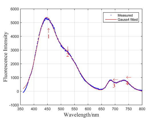
2.2. Laser-Induced Fluorescence of Rice Leaf (LIF)

According to the previous studies [35,36], the LIF intensity of rice leaf can be presented as,
I f ( λ i , λ e ) = φ λ I 0 ( λ e ) α ( λ e ) exp [ ( k 1 + k 1 ) x ] d x
which depends on the absorption of the leaf chlorophyll α ( λ e ) at the excitation wavelength λ e . By integrating over the whole leaf thickness x , I f ( λ i , λ e ) can be calculated with Equation (2) where I 0 ( λ e ) is the intensity of the excitation wavelength, and λ i is the fluorescence emission wavelength. The parameter φ λ represents the fluorescence efficiency. A LIF system [37] with a wavelength of 355 nm was used in this work to analyze and monitor the fluorescence spectrum of the rice leaf. This excitation laser source was generated by a 1064 nm Nd:YAG and its second and third harmonic generation. The repetition frequency was 20 Hz. The output power was 1.5 mJ and the width per pulse was 5 ns. The fluorescence spectrum range is 300 nm to 800 nm with a resolution of 0.5 nm, which is collected by an ICCD camera. Peak fitting with four Gaussian models was conducted to derive the fluorescence intensities at 450 nm, 510 nm, 685 nm, and 740 nm of the fluorescence spectrum. An example is shown in Figure 1.

2.3. Materials and the Design of Experiments

Experimentation in this study was conducted in Suizhou City, Hubei Province, China (113°13′26.52″E, 31°39′0.94″N). This area is a part of the Jianghan Plain which belongs to the subtropical monsoon zone. Its climate is mild and has a mean precipitation of 856 mm to 1070 mm and a temperature of 15.5 °C [38]. The type of cultivated land is paddy soil which contains abundant organic matters useful for plant growth. The rice variety was Yongyou 4949 which was seeded on 27 April 2014 and then transplanted into the experimental fields on 1 June 2014. Samples were the second leaves from the rice top, which were collected on 16 July 2014 (in booting stage) and 1 August 2014 (in heading stage). The samples size in each stage was 120 in this experiment. Six levels of urea fertilizer (0 kg/ha, 189 kg/ha, 229.5 kg/ha, 270 kg/ha, 310.5 kg/ha, and 351 kg/ha) were applied. Identical cultivation conditions were repeated in three fields. The fields were randomly designed and fertilized as follows: the total fertilizer of 30% as basic fertilization, 20% in booting stage, 25% in tillering stage, and 25% in heading stage.
In order to strictly control the laboratory conditions during the measurement, the laboratory was constructed as a dark room with little light except for that coming from the computer. Additionally, the incident angle of the laser beam was perpendicular to the leaf surface and kept constant along with the measuring distance. Moreover, the laser spot with a diameter of 10 mm resided on the leaf surface completely. The characteristic spectra of each sample, including the reflectance and LIF, were measured along the major axis of the leaf base at approximately one fourth, one half, and three fourths. At the same measurement position, five waveforms were collected. Thus, there are 15 waveforms were conducted in one leaf. The characteristic spectra of each sample were the average of these 15 waveforms. After spectra collection each sample was cut into pieces and then weighted as the fresh matters. Part of the fresh matter was put into a stove to dry at 105 °C for half an hour and then at 70 °C until it acquired the constant weight. The dry leaves were then used for LNC measurement with a chemical extraction solvent called the Kjeldahl analysis method [39]. Results were expressed as mg·nitrogen·g−1 leaf dry matter.

3. Data Analysis

A total of 36 input variables were used to model the relationship between the LNC and the spectra. Among them, 32 reflectance intensity values measured by a 32-channel HSL system [34] and four LIF peaks found in the fluorescence spectrum were included [37]. Several variables of these 32 reflectance intensities might be poorly related to LNC and could thus be removed without decreasing the regression accuracy. By using an iteration process and a feature extraction method (Section 3.2), it is necessary and feasible to select useful band combinations for LNC estimation based on the determination coefficient R2. Furthermore, four LIF discrete peaks were used to model the relationship with rice LNC in two forms: one is four LIF peaks (around 450 nm, 510 nm, 685 nm and 740 nm) as direct inputs and the other is two LIF indices (developed integrating bands of blue/red and blue/far-red) such as the normalized difference vegetation index (NDVI) describe in Equation (3). The latter was utilized to fuse more fluorescence properties into the regression models of rice LNC.
N D V I f l u o r e s c e n c e = F b l u e F r e d   o r   f a r _ r e d F b l u e + F r e d   o r   f a r _ r e d
Datasets from each growing stage were randomly separated into two parts: 80% for the calibration set and 20% for the validation set. During the process of data analysis, LNC was first associated with spectral data, including HSL and LIF, and then the models that performed well (with a larger R2) in LNC estimation would be tested based on the validation sets.

3.1. Regression Methods

3.1.1. Support Vector Machines (SVMs) Regression

According to Vapnick’s theory [40], SVM was actually to find a hyper-plane which could separate all classes. The final function of this plane was described as Equation (4):
f ( x ) = s i g n [ v i K ( x , y ) + b ]
K ( x , y ) = exp ( γ | x y | 2 )
where v i was the parameter which determines the support vector. Parameter b was a scalar threshold. Instead of calculating a dot product, the kernel function (K(x, y)) was used in Equation (4). In this study, the commonly used radial basis function (RBF, Equation (5)) was adopted as a kernel function of SVMs. To use a SVM for regression problems, Vapnick then specified a limitation of the regression error by a ε function. A small ε corresponded to a small regression error. The accuracy of SVM regression mainly depended on optimizing the penalty parameter (c) and the kernel parameter ( γ ), which were selected from the following sets: (−5, −4, …, 0, …, 4, 5) and (−10, −9, …, 0, …, 9, 10). The selection of these two parameters was based on the gridding method. They were optimized successively until a high R2 of estimation models was obtained.

3.1.2. Partial Least Squares (PLS)

PLS, based on principal component analysis (PCA), was first introduced by Wold et al. [41]. PLSR was the PLS approach in its simplest form to relate two data matrices, namely the input variables (X) and the responding variables (Y). PLSR could determine a linear relationship between X and Y by decomposing and screening data matrices simultaneously with a few independent principal components (PCs). These data matrices could be noisy, collinear, and incomplete.
Y λ = a 0 + a 1 S 1 λ + a 2 S 2 λ + ... + a n S n λ
where a n was the regression coefficient obtained by the linear regression of S n λ versus Y λ in a calibration iteration process, and S n λ was the score of the nth principal component at spectral band λ . The basic principle of PLSR will not be introduced in this paper, but further information can be found in Wold S. et al. [23].

3.1.3. Artificial Neural Networks (ANNs)

In this study, feed forward neural networks (NNs) were used. The NNs consisted of an input layer, a hidden layer and an output layer. The nodes in the input layer represented the reflectance and LIF spectrum gained by using the HSL and LIF system. The ANNs were created, trained, and implemented by using the BP-NN and RBF-NN toolbox of Matlab software. The ANNs were trained iteratively to minimize the mean square error (MSE) between the network outputs and the rice LNC. In each BP-NN iteration, the network weights ( w i ) and biases ( β i ) were adjusted along with the gradient decrease of the MSE. The transformation T in Equation (7) was a nonlinear activation function which could process this iteration and provide an output value y of this network.
y = T ( i = 1 n w i X i + β i )
In the present work, a minimum MSE of 10−3, a minimum gradient of 10−6 and a maximum iteration number (epochs) of 50 were adopted. Meeting any of these conditions, the ANN’s training process would stop. The spread of the radial basis network was 5. The larger the spread was, the smoother the function approximation would be [30,42].

3.2. Re-Ranking Wavelength Method

According to the algorithm of Huang, R. and M. He [43], a feature weighting method could remove the low correlation bands with the LNC. This method was based on a pairwise reparability criterion and matrix analysis. There were mainly two steps to conduct. The first step was to assume that the spectral data could be separated into m classes ( c = 1 , 2 , 3 ... m ), and the criterion of subset D was called the divergence of the cth class. Given that the first principal components contain the most information of the data, the modified D was calculated by Equation (8), as follows:
D = i = 1 n α × D ( i )
where α was the function related to the ith eigenvalue of the correlation matrix of the cth class. An eigenvector matrix element of the correlation matrix of the cth class was E λ j . A significant coefficient of the band λ corresponding to class c (denoted by η c ( λ ) ) could be presented as follows:
η c ( λ ) = 1 n j = 1 n μ j ( E λ j ) 2    ( j = 1 , 2 , ... , n )
The coefficient η c ( λ ) was ranked in a descending sequence. Parameter μ j represented a divergence ratio of the jth channel (the number of the channel was n), which could be calculated using Equation (10),
μ j = D ( j ) D
The second step of this method was to calculate the feature weight w ( λ ) of wavelength λ . The weight could be obtained by seeking the channel position p c λ in the sequence η c ( λ ) according to Equation (11)
w ( λ ) = 1 n c = 1 m ( n p c λ + 1 )
Spectral data was re-ranked based on feature weight w ( λ ) . Then optimal channel combinations were selected for the LNC estimation by comparing the determination coefficient R2.

4. Results and Discussion

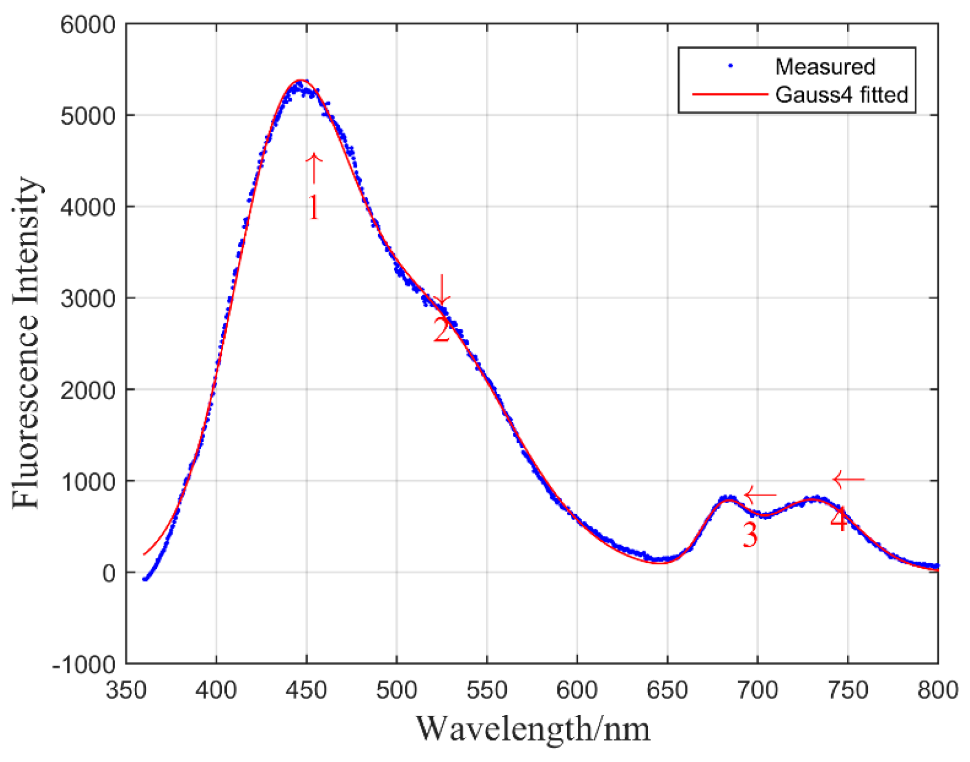
4.1. LNC Estimation Using Reflectance Spectra Based on Different Regression Methods

Figure 2 shows the coefficient of determination (R2) and the 1:1 relationship by using different regression methods between the observed and estimated LNC based on reflectance spectra. The maximum R2 of each method is plotted in the figures. The results show that these regression methods are useful for estimating rice LNC. Generally, the R2 values of regression models with different methods are greater than 0.7, that is, >0.9 with SVMs and RBF-NNs, >0.8 with BP-NNs and >0.7 with PLS.
Whether in booting or heading stages, SVM shows great potential in rice LNC estimation, whose maximum R2 can be more than 0.9 (0.963 in the booting stage with RMSE = 0.093 and 0.932 in the heading stage with RMSE = 0.1). The RMSE can be calculated by Equation (12), where X o b s e r v e d , i is the measured LNC, X m o d e l e d , i is the retrieved LNC, and N is the number of samples.
R M S E = i = 1 N ( X o b s e r v e d , i X m o d e l e d , i ) 2 n
Moreover, the estimated LNCs using the SVM at a low nitrogen content level (with a boundary of about 3.3 mg/g) are located at the left of the 1:1 line, which means that SVMs model higher values of LNC than the observed values. However, this phenomenon does not appear any more at a high nitrogen content level, where, conversely, the estimated LNC is lower than the observed LNC. Compared with the SVM method, the estimated LNC values modeled by RBF-NNs are dispersed over both sides of the 1:1 line, and some estimated values are even located on the 1:1 line. These results indicate that retrieval models with RBF-NNs are more reliable in LNC estimation. The estimated LNC values regressed by BP-NNs are distributed separately on the 1:1 line, and they show a relatively weaker relationship between the observed LNC and the estimated values, as does the PLS method. Additionally, the maximum R2 values of regression models obtained by using BP-NNs (0.889 in the booting stage and 0.856 in the heading stage) are lower than those obtained by using RBF-NNs (R2 = 0.979 in the booting stage and R2 = 0.957 in the heading stage). The maximum R2 values of PLS models in the booting and heading stages are 0.845 and 0.811, respectively. We find that the reflectance spectrum becomes insensitive in predicting chlorophyll concentrations when the LNC is high. This result is consistent with the findings of Eitel et al. [44], who fused the structural and biochemical information obtained from the green terrestrial LiDAR (light detection and ranging) scanning (TLS) to estimate the nitrogen status of winter wheat. Erdle et al. [45] also compared the active and passive sensors which were used to discriminate nitrogen status, and they found that a saturation effect with the increase of the LNC exists. The saturation effects may be caused by the changes of the photosynthetic photon flux density, by which several pigments of the plant can be affected.
In the study of Du et al. [34], SVMs were adopted to retrieve rice LNC, and they found that the R2 values of LNC retrieval models could become greater than 0.7 when all wavelengths were used as the input variables. In this study, all wavelengths were ranked on the basis of the corresponding feature weights before the LNC estimation. Then some of these wavelengths were chosen as the model inputs through an iteration process. For SVMs, RBF-NNs, BP-NNs and PLS, the retrieval models can be used to estimate the LNC in the validation set at a high precision in the order of RBF-NNs > SVMs > BP-NNs > PLS. Using SVMs for LNC retrieval, a kernel function called RBF was adopted, which was also used in the RBF-NNs. This result indicated that SVMs and RBF-NNs with a RBF function performed well in mapping rice LNC; thus, they are potentially effective methods in remote sensing techniques for rice LNC monitoring. The result also indicated that a non-linear relationship might exist between the LNC and reflectance spectra at different wavelengths. In addition, the running times exhibited a different order. We analyzed the data with a computer with an Intel (R) Core (TM) i7-3770, CPU @ 3.4 GHz (Lenovo, Wuhan, China). The RAM was 8 GB, and the system was Windows 7 (32 bit). In particular, the SVM-based model required the longest running time (5358.2 s), and PLSR was the fastest method (72.2 s). These results suggested how to find a suitable method for LNC estimation in practice, such as the design of a portable instrument with high accuracy and the development of a computer software program.

4.2. LNC Estimation Using Reflectance Spectrum and Reflectance + Fluorescence Spectrum

As mentioned in Section 2.3, the spectrum of LIF was closely correlated with the LNC and the chlorophyll contents in green plants; thus, it could be an essential indicator for biochemistry parameters. Fluorescence ratios (F740/F685 and F685/F525) were widely utilized for the estimation of the nitrogen status and for the diagnosis of crop growth because of their simplicity in measurement and interpretation [11,46]. However, studies of Yang Jian et al. [47] indicated that these fluorescence ratios were insensitive to the rice LNC. On the contrary, the rice LNC was closely correlated with the intensity of the fluorescence peaks (F450, F685 and F740). In this study, LIF spectra were utilized to estimate rice LNC in two forms: one was four peaks at wavelengths of 450 nm, 610 nm, 685 nm and 740 nm and the other was two indices calculated like the NDVI, such as (F450 − F685)/(F450 + F685) and (F450 − F740)/(F450 + F740). The maximum R2 values and the wavelengths applied to the LNC estimation with four regression algorithms in two growing stages were listed in Table 1.
The RBF-based SVM regression for LNC estimation relies on two parameters (c and γ ), which are selected through the grid screening method. This method is a long, time-consuming process, but it can obtain a relatively good result in these two different stages. Namely, the SVM method can yield a maximum R2 (> 0.9) and the RMSE is approximately 0.1 when using the reflectance spectra. Combined with the fluorescence spectral data in the form of four peaks directly, the maximum R2 can reach 0.966 in the booting stage and 0.937 in the heading stage; however, these values almost remain unchanged when the reflectance-based spectrum is considered. In addition, both fluorescence indices (F450 − F685)/(F450 + F685) and (F450 − F740)/(F450 + F740) have not improved the R2 and have even decreased in the process of LNC estimation while SVMs are used. Apart from the fact that BP-NNs have a lower R2 than SVMs and RBF-NNs, ANNs (BP-NNs and RBF-NNs) yield the same results which are consistent with SVMs when they are used for rice LNC estimation on the basis of fluorescence data in two stages.
PLSR is a method focused on modeling a linear relationship between the rice LNC and spectral variables. Among these four regression algorithms, PLSR is the weakest method in the LNC estimation of rice, and it exhibits a poorer performance, yielding R2 values of 0.845 and 0.811 in the booting and heading stages, respectively. However, PLSR links rice LNC and the spectral inputs with a relatively higher R2 by adding the fluorescence variables instead of using reflectance-based data only. In the booting stage R2 = 0.845, RMSE = 0.296 by using reflectance spectra; and R2 = 0.887, RMSE = 0.26 by combining the LIF index (F450 and F740). In the heading stage R2 = 0.811, RMSE = 0.203 by using reflectance spectra; and R2 = 0.874, RMSE = 0.194 by combining the LIF index (F450 and F740). Although the model performance has been improved slightly in this way, these results suggest that the LIF data, which is related to the chlorophyll contents in leaves, may be a reliable indicator to monitor the photosynthesis of crops, especially the index developed by integrating fluorescence intensities of 450 and 740 nm.

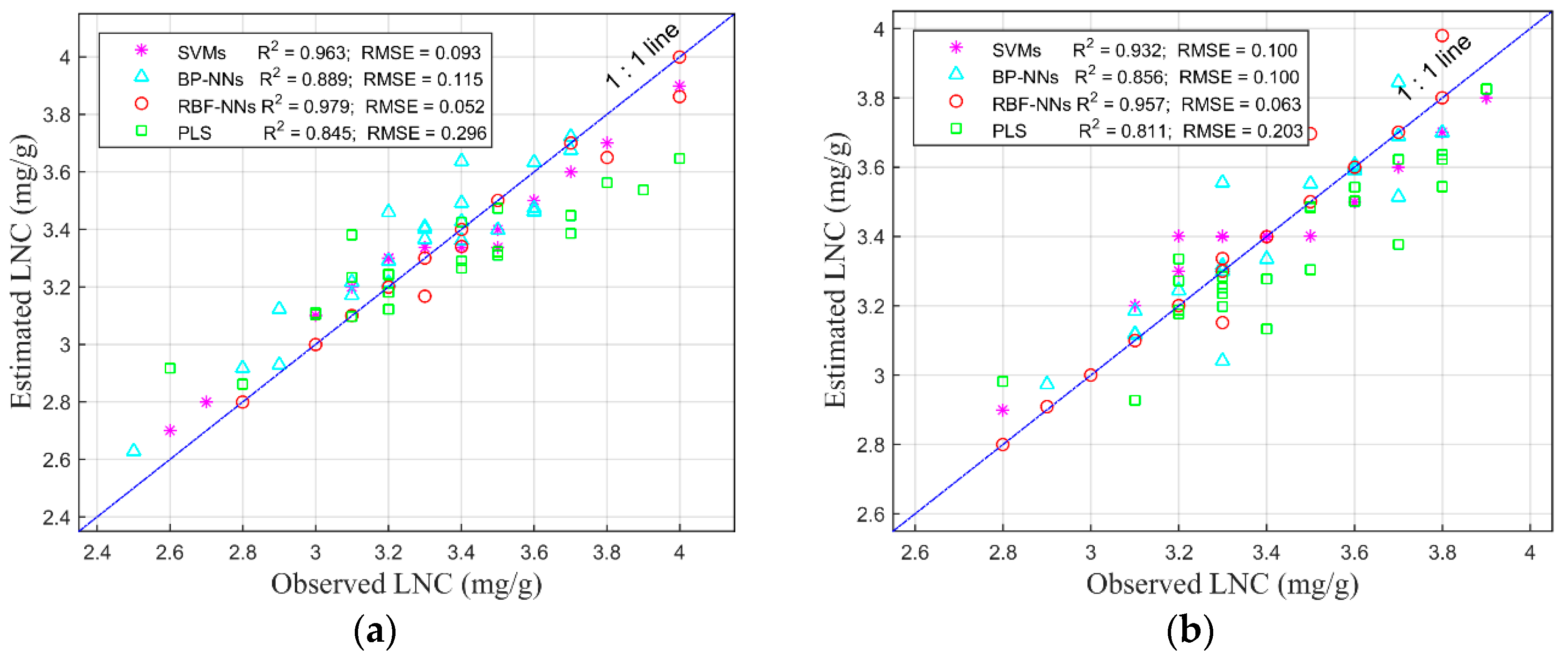
4.3. Band Combinations Based on HSL Data for Rice LNC Estimation

Although more wavelengths can provide additional informative features about the crops’ status, some of these wavelengths and input variables may be poorly correlated with rice LNC. Thus, the selection of key inputs of LNC retrieval models is an essential task in the remote sensing of crops’ growing stages and biochemistry parameters, such as nitrogen. In Section 3.2, all of the 32 wavelengths were re-ranked on the basis of their corresponding feature weights. Different band combinations (wavelengths showed in Table 1) were then conducted to estimate the rice LNC. Figure 3 shows the results obtained by using four regression methods, respectively, which indicate that for these methods, the values of R2 generally exhibit an increasing trend while the number of bands increases. Figure 3 also illustrates that approximately less than 17 variables (bands) with an R2 of >0.7 are sufficient to estimate the rice LNC. These 17 bands lie in the visible and near-infrared range (538 nm to 910 nm), which composes the working wavelength of the HSL system. In some bands of this spectral range, the light is strongly absorbed by chlorophyll in green plants, which is a sensitive indicator of the LNC. More details about the bands’ range and their corresponding channels can be found in the study of Du et al. [34].
Furthermore, in these two stages, the higher values of R2 for a few bands (approximately 0.86 for two bands in the booting stage and, nearby, 0.9 for two bands in the heading stage) are gained by SVMs. With an increase of the band numbers, the values of R2 will increase correspondingly but the effect is not very evident. The solid lines in Figure 3 showed the increasing tendency. Compared with other methods, SVMs showed higher stability on modeling the relationship between the LNC and the reflectance spectra. Nevertheless, as discussed in Section 4.1, the modeling process of SVMs requires a long time to determine the optimal regression parameters. Therefore, SVMs are not a suitable choice for spectra collection in the field experiments.
Consistent with the results of Xia Yao et al. [4], our study revealed that the most informative feature wavelengths could vary in different growth stages and experimental conditions. Thus, further works need to be conducted in selecting and explaining new wavelengths for various experiments of LNC estimation, including different sites, experimental conditions and species. Xia Yao et al. [4] and Tian, Y.C. et al. [48] revealed that LNC models exhibited better and more stable performances in later stages than at the early stages. However, our study demonstrated that a better performance of the LNC estimation could be obtained in the early stage by using different methods. Except for BP-NNs, the R2 value in the later stage was lower than that in the early stage. The reason for such a result was mainly because the metabolism process of green plants in later stages became complex and nitrogen was greatly accumulated and remobilized by that point. These results were consistent with those demonstrated by the studies of Novoa, R. et al. [49] and Hamid et al. [50]. They found that the maximum nitrogen fertilization was accumulated in the tillering stage. Then, the metabolism process of green plants remained complex until the heading stage, when this complexity became even more obvious.
Obviously, the experiment in this study was conducted in the laboratory. Field measurements would be helpful and significant for farmers to manage nitrogen fertilization efficiently in practice. In the future, HSL and LIF data with high spatial and temporal resolutions might be collected from an airborne or satellite platform, as the passive remote sensing technology has been applied in practice, such as in the sensors MODIS and AVHRR.

5. Conclusions

Four different regression methods were applied to monitor rice LNC on the basis of reflectance and fluorescence spectra. The R2 and RMSE were utilized to demonstrate the performance, advantages and robustness of these algorithms for LNC estimation. Results demonstrated that these four methods could be applied with high potential in rice LNC retrieval. SVMs and RBF-NNs exhibited a more accurate and stable capability than PLS and BP-NNs in modeling LNC with the reflectance and LIF spectra. LIF information, including fluorescence peaks and indices, was used as a potential indicator for the monitoring of rice LNC. Given that the forms of LIF spectra used in this study were simple, and the improvement of R2 in the LNC estimation models was not evident, more effective LIF index forms for LNC estimation should be found. As this study was performed with just one species and under strictly controlled laboratory conditions, limitations certainly existed regarding wider application in other sites and varieties. Thus, a simulation research based on a physical radiative transfer model or the principle of LIF of chlorophyll should be considered. In addition, except for the parametric regression analysis, the non-parametric and even hybrid methods of both of them may be additional good choices for LNC estimation in the future.

Acknowledgments

This work was supported by National Natural Science Foundation of China (Grant No. 41127901), Program for Innovative Research Team in University of Ministry of Education of China (Grant No. IRT1278), Natural Science Foundation of Hubei Province, China (Grant No. 2015CFA002). Open Research Fund of State Key Laboratory of Information Engineering in Surveying, Mapping and Remote Sensing (Grant No. 15R01).

Author Contributions

Lin Du and Wei Gong conceived and designed the experiments; Lin Du, Shuo Shi, Jian Yang and Jia Sun performed the experiments; Shuo Shi and Lin Du analyzed the data; Jian Yang and Jia Sun contributed reagents/materials/analysis tools; Lin Du wrote the paper.

Conflicts of Interest

The authors declare no conflict of interest.

Abbreviations

The following abbreviations are used in this manuscript:
LNCLeaf Nitrogen Content
LIFLaser-induced Fluorescence
HSLHyperspectral LiDAR
SVMsSupport Vector Machines
PLSRPartial Least Squares Regression
PLSPartial Least Squares
ANNsArtificial Neural Networks
RBF-NNsRadial Basis Function Neural Networks
BP-NNsBack Propagation Neural Networks

References

  1. Johnson, L.F. Nitrogen influence on fresh-leaf NIR spectra. Remote Sens. Environ. 2001, 78, 314–320. [Google Scholar] [CrossRef]
  2. Curran, P.J.; Dungan, J.L.; Peterson, D.L. Estimating the foliar biochemical concentration of leaves with reflectance spectrometry: Testing the Kokaly and Clark methodologies. Remote Sens. Environ. 2001, 76, 349–359. [Google Scholar] [CrossRef]
  3. Kergoat, L.; Lafont, S.; Arneth, A.; Le Dantec, V.; Saugier, B. Nitrogen controls plant canopy light-use efficiency in temperate and boreal ecosystems. J. Geophys. Res. Biogeosci. 2008, 113, 1–19. [Google Scholar] [CrossRef]
  4. Yao, X.; Huang, Y.; Shang, G.Y.; Zhou, C.; Cheng, T.; Tian, Y.C.; Cao, W.X.; Zhu, Y. Evaluation of Six Algorithms to Monitor Wheat Leaf Nitrogen Concentration. Remote Sens. 2015, 7, 14939–14966. [Google Scholar] [CrossRef]
  5. Nevalainen, O.; Hakala, T.; Suomalainen, J.; Mäkipää, R.; Peltoniemi, M.; Krooks, A.; Kaasalainen, S. Fast and nondestructive method for leaf level chlorophyll estimation using hyperspectral LiDAR. Agric. Forest Meteorol. 2014, 198, 250–258. [Google Scholar] [CrossRef]
  6. Woodhouse, I.H.; Nichol, C.; Sinclair, P.; Jack, J.; Morsdorf, F.; Malthus, T.J. A multispectral canopy LiDAR demonstrator project. IEEE Geosci. Remote Sens. Lett. 2011, 8, 839–843. [Google Scholar] [CrossRef]
  7. Niu, Z.; Xu, Z.; Sun, G.; Huang, W.; Wang, L.; Feng, M.; Li, W.; He, W.B.; Gao, S. Design of a New Multispectral Waveform LiDAR Instrument to Monitor Vegetation. IEEE Geosci. Remote Sens. Lett. 2015, 12, 1506–1510. [Google Scholar]
  8. Wallace, A.; Nichol, C.; Woodhouse, I. Recovery of forest canopy parameters by inversion of multispectral LiDAR data. Remote Sens. 2012, 4, 509–531. [Google Scholar] [CrossRef]
  9. Apostol, S.; Viau, A.A.; Tremblay, N. A comparison of multiwavelength laser-induced fluorescence parameters for the remote sensing of nitrogen stress in field-cultivated corn. Can. J. Remote Sens. 2007, 33, 150–161. [Google Scholar] [CrossRef]
  10. Maxwell, K.; Johnson, G.N. Chlorophyll fluorescence—A practical guide. J. Exp. Bot. 2000, 51, 659–668. [Google Scholar] [CrossRef] [PubMed]
  11. Zarco-Tejada, P.J.; Miller, J.R.; Mohammed, G.H.; Noland, T.L. Chlorophyll fluorescence effects on vegetation apparent reflectance: I. Leaf-level measurements and model simulation. Remote Sens. Environ. 2000, 74, 582–595. [Google Scholar] [CrossRef]
  12. Chappelle, E.W.; Wood, F.M.; McMurtrey, J.E.; Newcomb, W.W. Laser-induced fluorescence of green plants. 1: A technique for the remote detection of plant stress and species differentiation. Appl. Opt. 1984, 23, 134–138. [Google Scholar] [CrossRef] [PubMed]
  13. Subhash, N.; Mohanan, C. Laser-induced red chlorophyll fluorescence signatures as nutrient stress indicator in rice plants. Remote Sens. Environ. 1994, 47, 45–50. [Google Scholar] [CrossRef]
  14. Alekseyev, V.; Babichenko, S.; Sobolev, I. Control and signal processing system of hyperspectral FLS LiDAR. In Proceedings of the 2008 11th International Biennial Baltic Electronics Conference, Tallinn, Estonia, 6–8 October 2008; pp. 349–352.
  15. Haboudane, D.; Tremblay, N.; Miller, J.R.; Vigneault, P. Remote estimation of crop chlorophyll content using spectral indices derived from hyperspectral data. Geosci. Remote Sens. IEEE Trans. 2008, 46, 423–437. [Google Scholar] [CrossRef]
  16. Schlemmer, A.G.M.; Schepers, J.; Ferguson, R.; Peng, Y.; Shanahan, J.; Rundquist, D. Remote estimation of nitrogen and chlorophyll contents in maize at leaf and canopy levels. Int. J. Appl. Earth Obs. Geoinformation 2013, 25, 47–54. [Google Scholar] [CrossRef]
  17. Zarco-Tejada, P.J.; Berjón, A.; López-Lozano, R.; Miller, J.; Martín, P.; Cachorro, V.; González, M.R.; Frutos, D.A. Assessing vineyard condition with hyperspectral indices: Leaf and canopy reflectance simulation in a row-structured discontinuous canopy. Remote Sens. Environ. 2005, 99, 271–287. [Google Scholar] [CrossRef]
  18. Lichtenthaler, H.K.; Miehe, J.A. Fluorescence imaging as a diagnostic tool for plant stress. Trends Plant Sci. 1997, 2, 316–320. [Google Scholar] [CrossRef]
  19. Stober, F.; Lichtenthaler, H.K. Characterization of the laser-induced blue, green and red fluorescence signatures of leaves of wheat and soybean grown under different irradiance. Physiol. Plant. 1993, 88, 696–704. [Google Scholar] [CrossRef]
  20. Hansen, P.; Schjoerring, J. Reflectance measurement of canopy biomass and nitrogen status in wheat crops using normalized difference vegetation indices and partial least squares regression. Remote Sens. Environ. 2003, 86, 542–553. [Google Scholar] [CrossRef]
  21. Song, S.; Gong, W.; Zhu, B.; Huang, X. Wavelength selection and spectral discrimination for paddy rice, with laboratory measurements of hyperspectral leaf reflectance. ISPRS J. Photogramm. Remote Sens. 2011, 66, 672–682. [Google Scholar] [CrossRef]
  22. Du, L.; Shi, S.; Yang, J.; Sun, J.; Gong, W. Estimation of leaf nitrogen content of rice using spectral indices and partial least squares regression based on hyperspectral LIDAR data. Unpublished Work. 2016. [Google Scholar]
  23. Wold, S.; Sjöström, M.; Eriksson, L. PLS-regression: A basic tool of chemometrics. Chemom. Intell. Lab. Syst. 2001, 58, 109–130. [Google Scholar] [CrossRef]
  24. Yu, K.; Li, F.; Martin, L.G.; Miao, Y.; Georg, B.; Chen, X.P. Remotely detecting canopy nitrogen concentration and uptake of paddy rice in the Northeast China Plain. ISPRS J. Photogramm. Remote Sens. 2013, 78, 102–115. [Google Scholar] [CrossRef]
  25. Farifteh, J.; Van der Meer, F.; Atzberger, C.; Carranza, E.J.M. Quantitative analysis of salt-affected soil reflectance spectra: A comparison of two adaptive methods (PLSR and ANN). Remote Sens. Environ. 2007, 110, 59–78. [Google Scholar] [CrossRef]
  26. Camps-Valls, G.; Luis, G.; Jordi, M.; Joan, V.; Julia, A.; Javier, C. Retrieval of oceanic chlorophyll concentration with relevance vector machines. Remote Sens. Environ. 2006, 105, 23–33. [Google Scholar] [CrossRef]
  27. Pal, M.; Mather, P.M. An assessment of the effectiveness of decision tree methods for land cover classification. Remote Sens. Environ. 2003, 86, 554–565. [Google Scholar] [CrossRef]
  28. Mantero, P.; Moser, G.; Serpico, S.B. Partially supervised classification of remote sensing images through SVM-based probability density estimation. Geosci. Remote Sens. IEEE Trans. 2005, 43, 559–570. [Google Scholar] [CrossRef]
  29. Mountrakis, G.; Im, J.; Ogole, C. Support vector machines in remote sensing: A review. ISPRS J. Photogramm. Remote Sens. 2011, 66, 247–259. [Google Scholar] [CrossRef]
  30. Samanta, B.; Al-Balushi, K.; Al-Araimi, S. Artificial neural networks and support vector machines with genetic algorithm for bearing fault detection. Eng. Appl. Artif. Intell. 2003, 16, 657–665. [Google Scholar] [CrossRef]
  31. Römer, C.; Bürling, K.; Hunsche, M.; Rumpf, T.; Noga, G.; Plümer, L. Robust fitting of fluorescence spectra for pre-symptomatic wheat leaf rust detection with support vector machines. Comput. Electron. Agric. 2011, 79, 180–188. [Google Scholar] [CrossRef]
  32. Gill, M.K.; Asefa, T.; Mariush, W.K.; Mckee, M. Soil moisture prediction using support vector machines 1. J. Am. Water Resour. Assoc. 2006, 42, 1033–1046. [Google Scholar] [CrossRef]
  33. Yang, X.; Huang, J.; Wu, Y.P.; Wang, W.J.; Wang, P.; Wang, X.; Huete, A.R. Estimating biophysical parameters of rice with remote sensing data using support vector machines. Sci. China Life Sci. 2011, 54, 272–281. [Google Scholar] [CrossRef] [PubMed]
  34. Du, L.; Gong, W.; Shi, S.; Yang, J.; Sun, J.; Zhu, B.; Song, S. Estimation of rice leaf nitrogen contents based on hyperspectral LIDAR. Int. J. Appl. Earth Obs. Geoinform. 2016, 44, 136–143. [Google Scholar] [CrossRef]
  35. Dahn, H.; Gunther, K.; Ludeker, W. Characterization of drought stress of maize and wheat canopies by means of spectral resolved laser induced fluorescence. EARSeL Adv. Remote Sens. 1992, 1, 12–19. [Google Scholar]
  36. Günther, K.; Dahn, H.G.; Lüdeker, W. Remote sensing vegetation status by laser-induced fluorescence. Remote Sens. Environ. 1994, 47, 10–17. [Google Scholar] [CrossRef]
  37. Yang, J.; Gong, W.; Shi, S.; Du, L.; Sun, J.; Zhu, B.; Ma, Y.; Song, S. Vegetation identification based on characteristics of fluorescence spectral spatial distribution. RSC Adv. 2015, 5, 56932–56935. [Google Scholar] [CrossRef]
  38. Stocker, T.; Qin, D.; Plattner, G.; Tignor, M.; Allen, S.; Boschung, J. Climate Change 2013: The Physical Science Basis; Intergovernmental Panel on Climate Change: Geneva, Switzerland, 2013. [Google Scholar]
  39. Wutzke, K.D.; Heine, W. A century of Kjeldahl’s nitrogen determination. Z. Med. Lab. 1984, 26, 383–388. [Google Scholar]
  40. Vapnick, V.N. Statistical Learning Theory; John Wiley and Sons Inc.: New York, NY, USA, 1998. [Google Scholar]
  41. Wold, S.; Ruhe, A.; Wold, H.; Dunn, W.J., III. The collinearity problem in linear regression. The partial least squares (PLS) approach to generalized inverses. SIAM J. Sci. Statist. Comput. 1984, 5, 735–743. [Google Scholar] [CrossRef]
  42. Paya, B.; Esat, I.; Badi, M. Artificial neural network based fault diagnostics of rotating machinery using wavelet transforms as a preprocessor. Mech. Syst. Process. 1997, 11, 751–765. [Google Scholar] [CrossRef]
  43. Huang, R.; He, M. Band selection based on feature weighting for classification of hyperspectral data. IEEE Geosci. Remote Sens. Lett. 2005, 2, 156–159. [Google Scholar] [CrossRef]
  44. Eitel, J.U.; Magney, T.S.; Vierling, L.A.; Brown, T.T.; Huggins, D.R. LiDAR based biomass and crop nitrogen estimates for rapid, non-destructive assessment of wheat nitrogen status. Field Crops Res. 2014, 159, 21–32. [Google Scholar] [CrossRef]
  45. Erdle, K.; Mistele, B.; Schmidhalter, U. Comparison of active and passive spectral sensors in discriminating biomass parameters and nitrogen status in wheat cultivars. Field Crops Res. 2011, 124, 74–84. [Google Scholar] [CrossRef]
  46. Živčák, M.; Olšovská, K.; Slamka, P.; Galambošová, J.; Rataj, V.; Shao, H.B.; Brestič, M. Application of chlorophyll fluorescence performance indices to assess the wheat photosynthetic functions influenced by nitrogen deficiency. Plant Soil Environ. 2014, 60, 210–215. [Google Scholar]
  47. Yang, J.; Shi, S.; Gong, W.; Du, L.; Ma, Y.; Zhu, B.; Song, S. Application of fluorescence spectrum to precisely inverse paddy rice nitrogen content. Plant Soil Environ. 2015, 61, 182–188. [Google Scholar] [CrossRef]
  48. Tian, Y.C.; Gu, K.J.; Chu, X.; Yao, X.; Cao, W.X.; Zhu, Y. Comparison of different hyperspectral vegetation indices for canopy leaf nitrogen concentration estimation in rice. Plant Soil 2014, 376, 193–209. [Google Scholar] [CrossRef]
  49. Novoa, R.; Loomis, R. Nitrogen and plant production. Plant Soil 1981, 58, 177–204. [Google Scholar] [CrossRef]
  50. Hamid, A. Efficiency of N uptake by wheat, as affected by time and rate of application, using N15-labelled ammonium sulphate and sodium nitrate. Plant Soil 1972, 37, 389–394. [Google Scholar] [CrossRef]
Figure 1. Example of a fluorescence spectrum and its approximation by a Gaussian model.
Remotesensing 08 00526 g001
Figure 2. R2 of estimation models and the 1:1 relationship between the observed LNC and those estimated using SVMs, ANNs (RBF-NN and BP-NN) and PLS in the (a) booting and (b) heading stages based on the reflectance spectra.
Remotesensing 08 00526 g002
Figure 3. Different band combinations with an R2 of >0.7 used for LNC estimation based on different regression methods in the (a) booting and (b) heading stages.
Remotesensing 08 00526 g003
Table 1. The maximum R2 and the wavelengths applied to LNC estimation with four regression algorithms in two growing stages of rice.
ModelsStagesReflectanceReflectance + Fluorescence (Peaks or Index)
Rmax2RMSEParametersWavelengths (nm)Rmax2RMSEParametersWavelengths (nm)
SVMsbooting0.9630.093c 1 = 0.707754 694 742 814 790 634 874 886 610 718 706 778 622 586 550Peaks 3 0.9660.092c = 0.707 γ = 0.008450 685
γ 2 = 1024Index 4 ----
heading0.930.104c = 0.707910 634 562 886 706 550 874 826 646Peaks 0.9370.099c = 0.5 γ = 0.000977685 740
γ = 1024Index 0.8990.103c = 0.707 γ = 1024450 & 740
BP-NNsbooting0.8890.115l 5 = 10682 766 754 742 826 862 634 898 598 610 718Peaks 0.8820.129l = 10510
Index 0.8930.09450 & 740
heading0.8560.099l = 10910 802 670 538 706 550 874 898 586 862 658 574Peaks 0.8530.117l = 10450 740
Index ---
RBF-NNsbooting0.9790.052s 6 = 5682 766 850 754 742 826 814 790 898Peaks 0.9590.076s = 5685
Index 0.9480.079450 & 685
heading0.9570.063s = 5910 634 598 886 538 790 622 898 646 586Peaks 0.9180.068s = 5450 510
Index 0.9270.071450 & 685
PLSbooting0.8450.296PCs 7 = 6682 850 754 838 802 634 658 730 646Peaks 0.8320.279PCs = 4450 685
Index 0.8870.26PCs = 5450 & 740
heading0.8110.203PCs = 6910 589 802 838 706 622 874 646 586 682 658 610 694Peaks 0.8670.196PCs = 5450 685
Index 0.8740.194PCs = 5450 & 740
1,2 Parameters in order to optimize the accuracy in SVM regression; 3 The LIF peaks at 450 nm, 510 nm, 685 nm and 740 nm; 4 The LIF indices developed with blue, red, and far-red bands using Equation (3); 5 The number of layers in BP-ANN analysis; 6 The spread of RBF in RBF-NN analysis; 7 The number of principal component (PCs) in PLSR analysis.

