
Particle Filter Approach for Real-Time Estimation of Crop Phenological States Using Time Series of NDVI Images


Abstract
:
1. Introduction
2. Methodology
2.1. Particle Filter (PF) Theory
2.2. Particle Filter Implementation
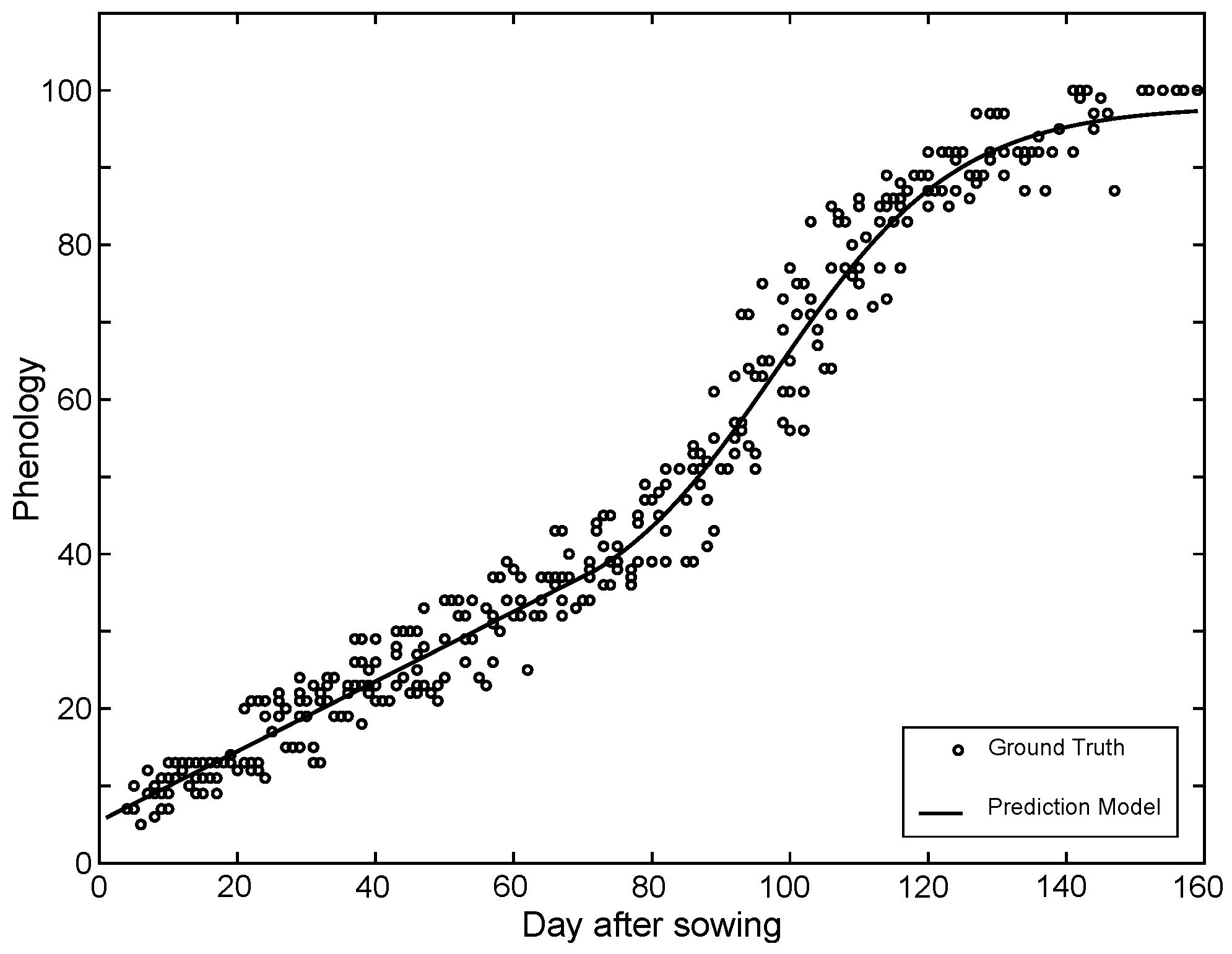
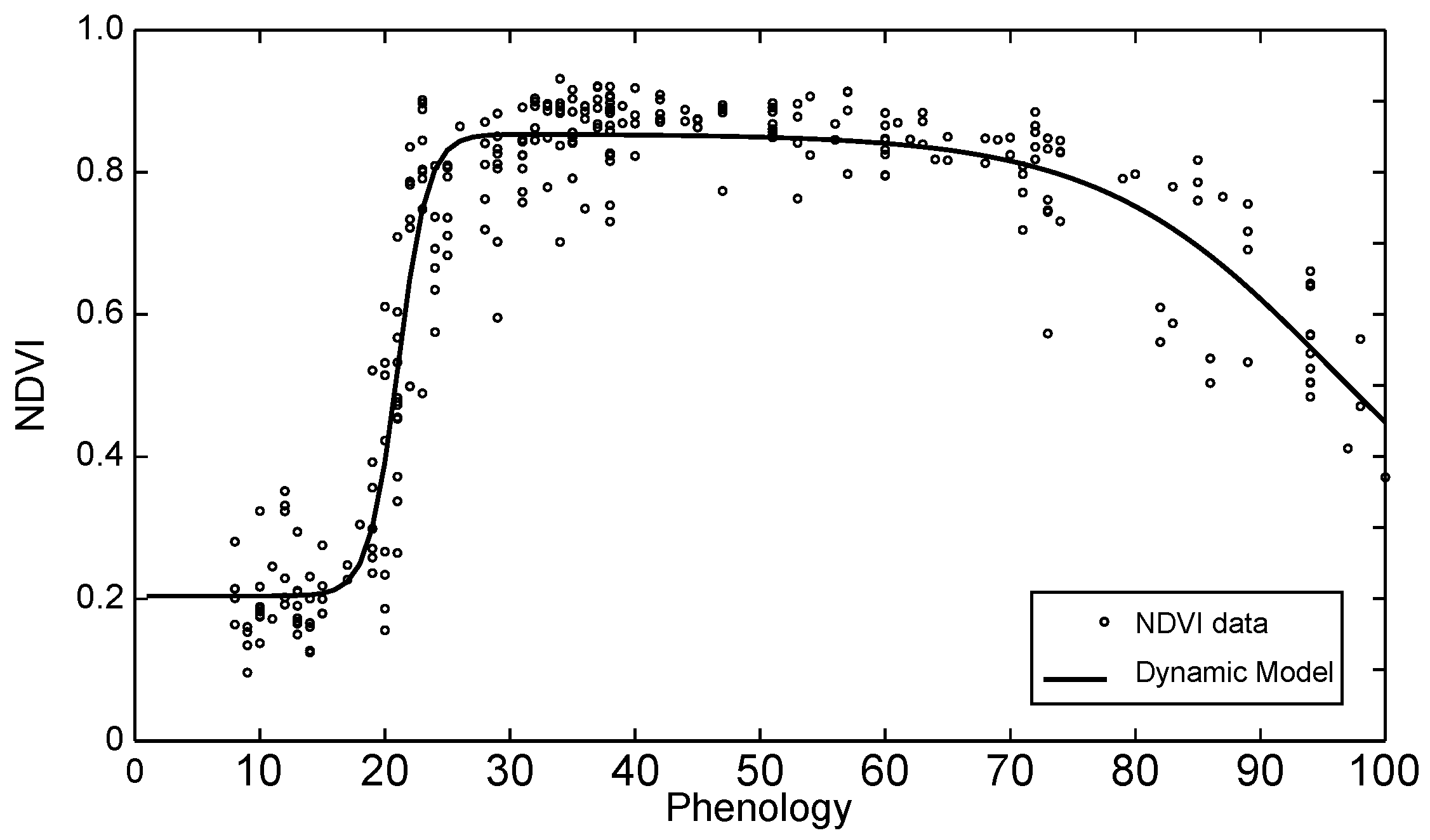
2.2.1. Crop Phenology Model
2.2.2. Observation Model
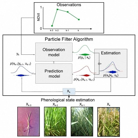
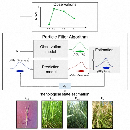
2.2.3. Estimation
3. Data Set and Test Site
4. Results
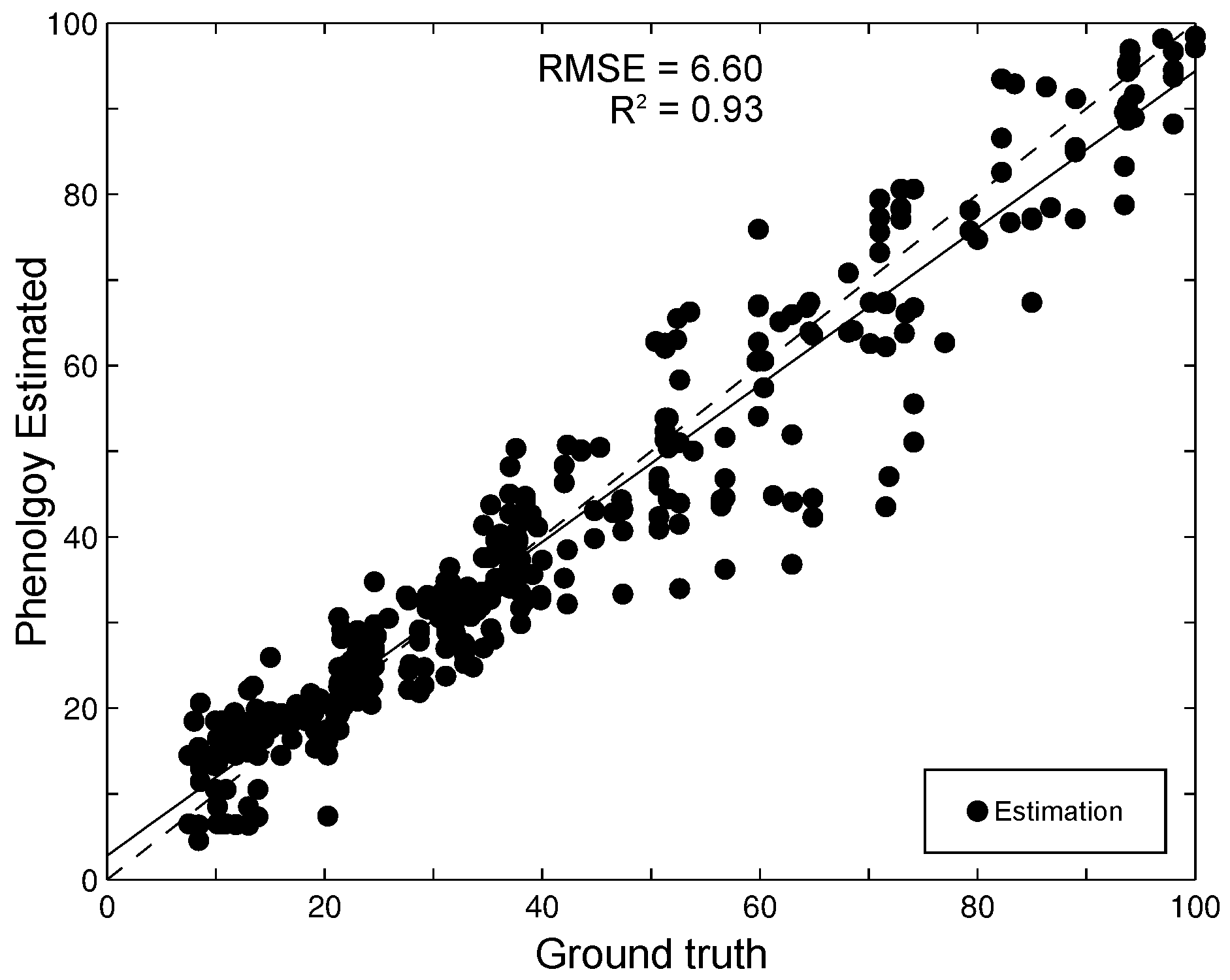
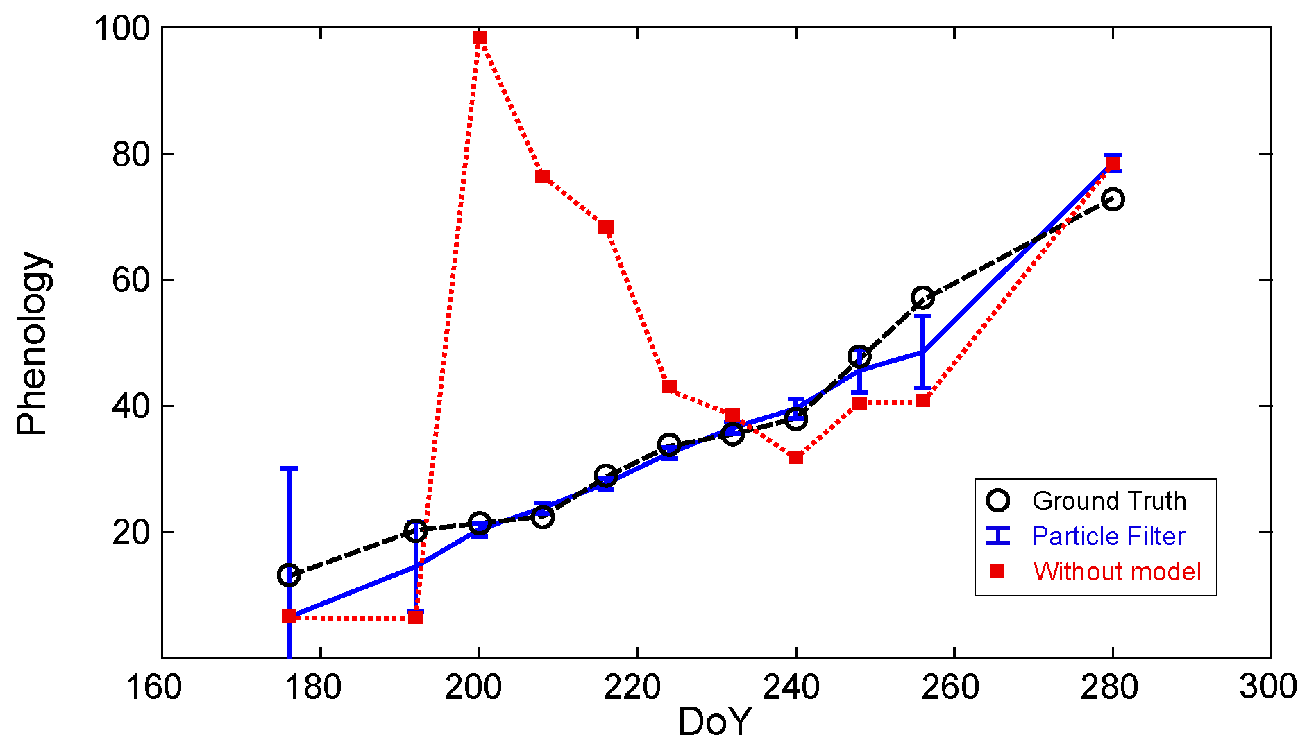
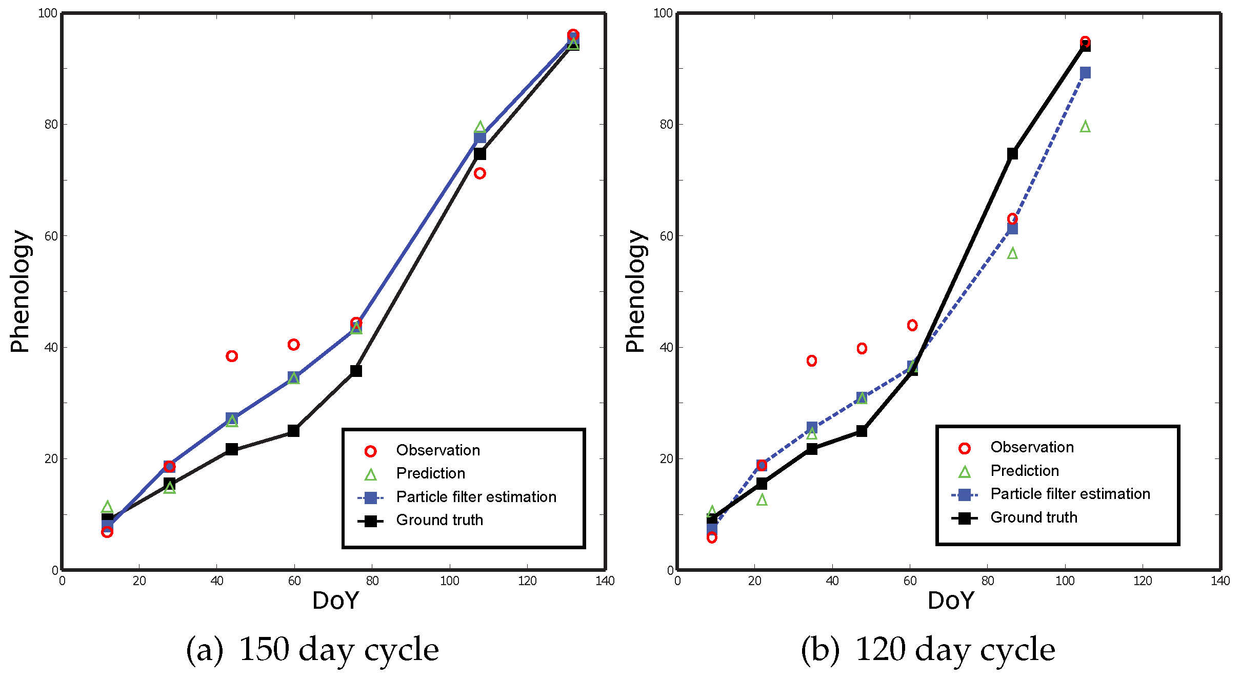
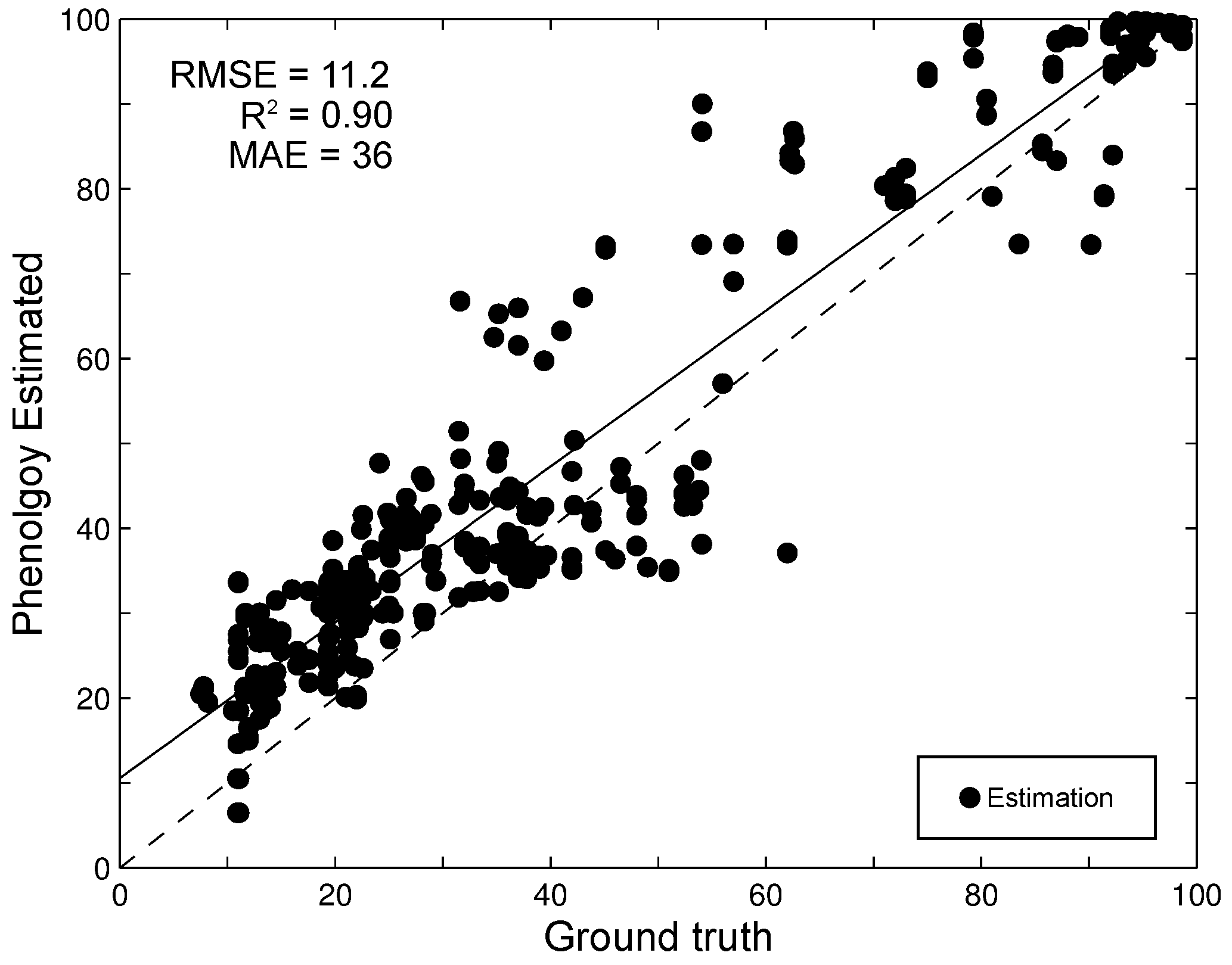
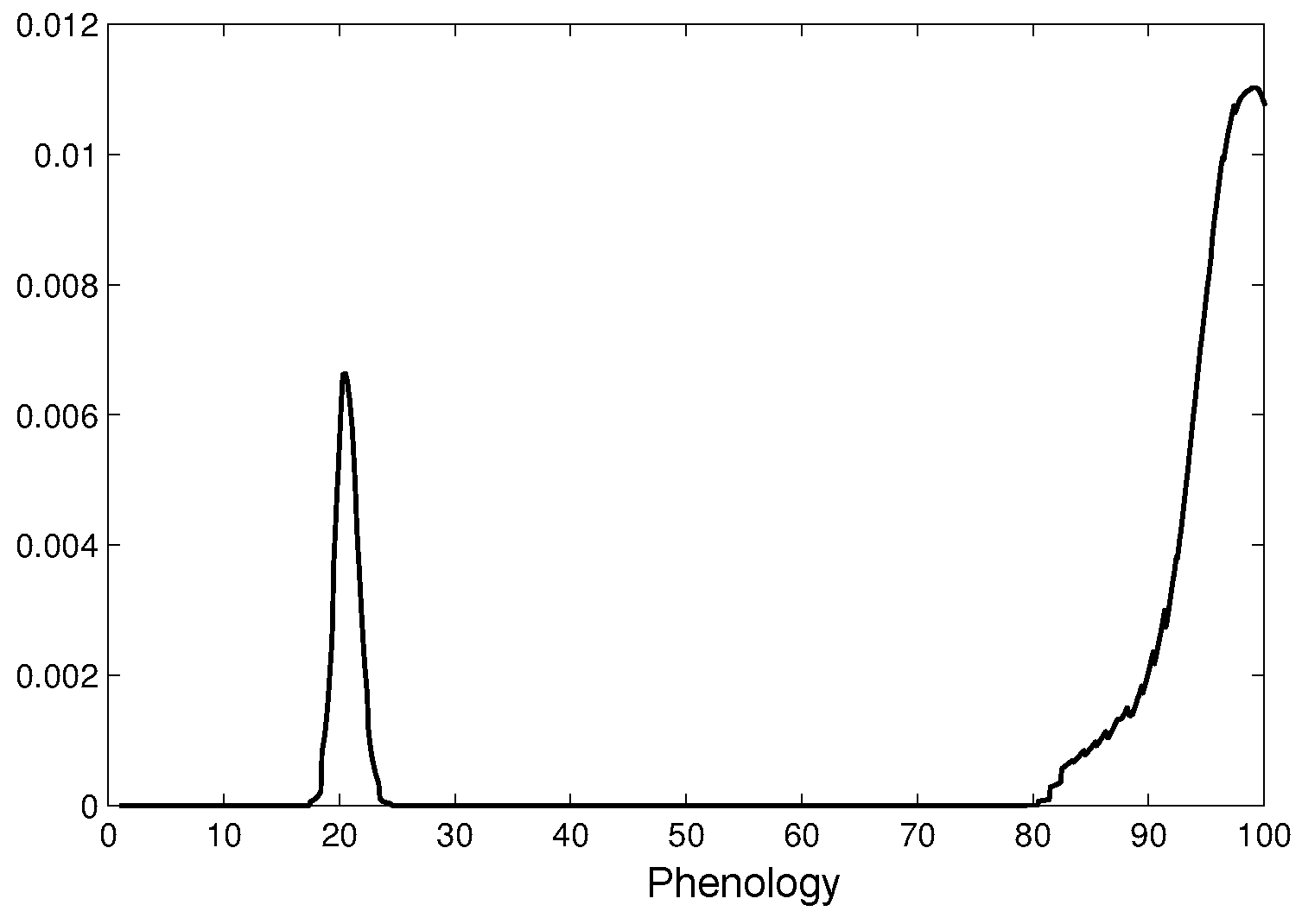
4.1. Phenological State Estimation
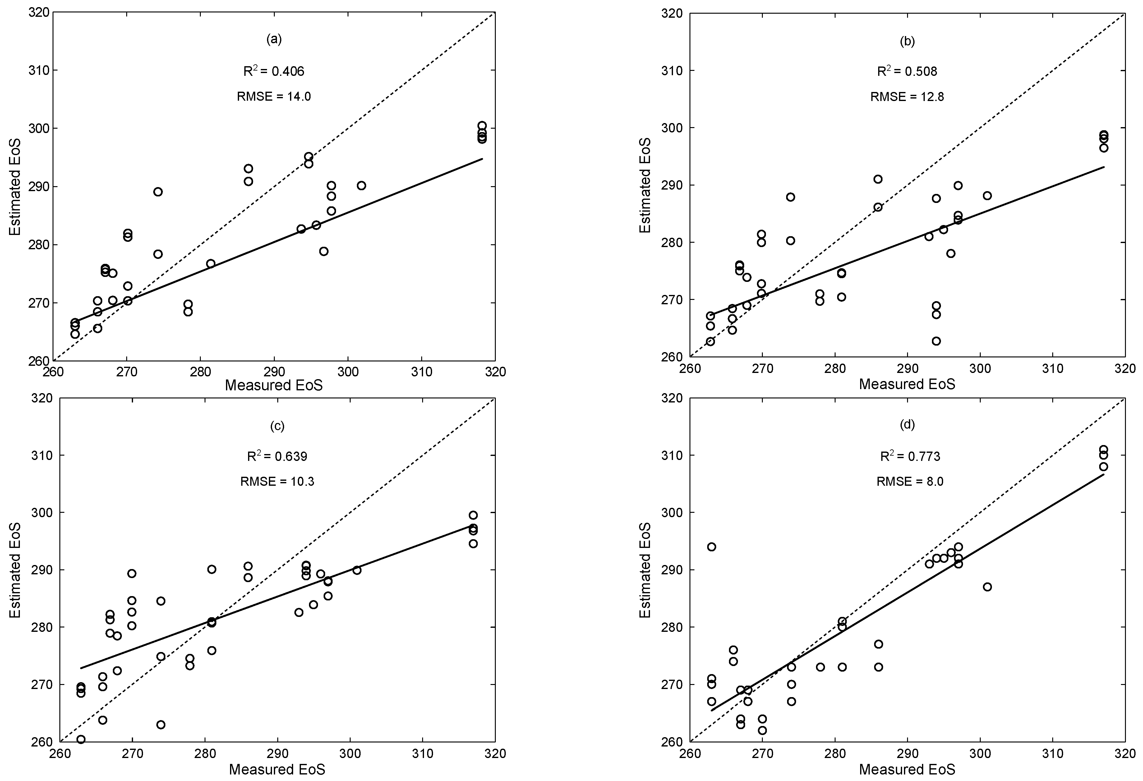
4.2. Prediction of Key Dates
4.3. Estimation over Other Types of Rice
5. Discussion
5.1. State Estimation and Prediction
5.2. Methodology Generalisation
5.3. Summary of Advantages
5.4. Perspectives and Future Research Lines
6. Conclusions
Acknowledgments
Author Contributions
Conflicts of Interest
References
- Islam, A.S.; Bala, S.K. Assessment of potato phenological characteristics using MODIS-derived NDVI and LAI information. GISci. Remote Sens. 2008, 45, 454–470. [Google Scholar] [CrossRef]
- Sakamoto, T.; Yokozawa, M.; Toritani, H.; Shibayama, M.; Ishitsuka, N.; Ohno, H. A crop phenology detection method using time-series MODIS data. Remote Sens. Environ. 2005, 96, 366–374. [Google Scholar] [CrossRef]
- Wardlow, B.D.; Kastens, J.H.; Egbert, S.L. Using USDA crop progress data for the evaluation of greenup onset date calculated from MODIS 250-meter data. Photogramm. Eng. Remote Sens. 2006, 72, 1225–1234. [Google Scholar] [CrossRef]
- Fan, H.; Fu, X.; Zhang, Z.; Wu, Q. Phenology-Based vegetation index differencing for mapping of rubber plantations using Landsat OLI data. Remote Sens. 2015, 7, 6041–6058. [Google Scholar] [CrossRef]
- Zhang, X.; Friedl, M.A.; Schaaf, C.B.; Strahler, A.H.; Hodges, J.C.; Gao, F.; Reed, B.C.; Huete, A. Monitoring vegetation phenology using MODIS. Remote Sens. Environ. 2003, 84, 471–475. [Google Scholar] [CrossRef]
- Jönsson, P.; Eklundh, L. Seasonality extraction by function fitting to time-series of satellite sensor data. IEEE Trans. Geosci. Remote Sens. 2002, 40, 1824–1832. [Google Scholar] [CrossRef]
- Van Dijk, A.; Callis, S.L.; Sakamoto, C.M.; Decker, W.L. Smoothing vegetation index profiles: An alternative method for reducing radiometric disturbance in NOAA/AVHRR data. Photogramm. Eng. Remote Sens. 1987, 53, 1059–1067. [Google Scholar]
- Jakubauskas, M.E.; Legates, D.R.; Kastens, J.H. Harmonic analysis of time-series AVHRR NDVI data. Photogramm. Eng. Remote Sens. 2001, 67, 461–470. [Google Scholar]
- Menenti, M.; Jia, L.; Azzali, S.; Roerink, G.; Gonzalez-Loyarte, M.; Leguizamon, S. Analysis of vegetation response to climate variability using extended time series of multispectral satellite images. In Remote Sensing Optical Observation of Vegetation Properties; Research Signpost: Trivandrum, India, 2010; pp. 131–163. [Google Scholar]
- Sakamoto, T.; Wardlow, B.D.; Gitelson, A.A.; Verma, S.B.; Suyker, A.E.; Arkebauer, T.J. A two-step filtering approach for detecting maize and soybean phenology with time-series MODIS data. Remote Sens. Environ. 2010, 114, 2146–2159. [Google Scholar] [CrossRef]
- White, M.A.; Nemani, R.R. Real-time monitoring and short-term forecasting of land surface phenology. Remote Sens. Environ. 2006, 104, 43–49. [Google Scholar] [CrossRef]
- Suwannachatkul, S.; Kasetkasem, T.; Chumkesornkulkit, K.; Rakwatin, P.; Chanwimaluang, T.; Kumazawa, I. Rice cultivation and harvest date estimation using MODIS NDVI time-series data. In Proceedings of the International Conference on Information and Communication Technology for Embedded Systems, Ayutthaya, Thailand, 23–25 January 2014; pp. 37–43.
- Viskari, T.; Hardiman, B.; Desai, A.R.; Dietze, M.C. Model-data assimilation of multiple phenological observations to constrain and predict leaf area index. Ecol. Appl. 2015, 25, 546–558. [Google Scholar] [CrossRef] [PubMed]
- Zhao, Y.; Chen, S.; Shen, S. Assimilating remote sensing information with crop model using Ensemble Kalman Filter for improving LAI monitoring and yield estimation. Ecol. Model. 2013, 270, 30–42. [Google Scholar] [CrossRef]
- Durrant-Whyte, H.; Bailey, T. Simultaneous localization and mapping: Part I. IEEE Robot. Autom. Mag. 2006, 13, 99–110. [Google Scholar] [CrossRef]
- Okuma, K.; Taleghani, A.; De Freitas, N.; Little, J.J.; Lowe, D.G. A boosted particle filter: Multitarget detection and tracking. In Computer Vision-ECCV 2004; Springer: Prague, Czech Republic, 2004; pp. 28–39. [Google Scholar]
- Jackson, R.D. Remote sensing of vegetation characteristics for farm management. Proc. SPIE 1984, 475, 81–96. [Google Scholar]
- Kalman, R.E. A new approach to linear filtering and prediction problems. J. Basic Eng. 1960, 82, 35–45. [Google Scholar] [CrossRef]
- Doucet, A.; Godsill, S.; Andrieu, C. On sequential Monte Carlo sampling methods for Bayesian filtering. Stat. Comput. 2000, 10, 197–208. [Google Scholar] [CrossRef]
- Kalos, M.H.; Whitlock, P.A. Monte Carlo Methods; John Wiley & Sons: Weinheim, Germany, 2008. [Google Scholar]
- Bergman, N. Recursive Bayesian Estimation. Ph.D. Dissertation, Department of Electrical Engineering, Linköping University, Linköping, Sweden, 1999. [Google Scholar]
- Ghosh, M.; Mukhopadhyay, N.; Sen, P.K. Sequential Bayesian Estimation; John Wiley & Sons: Hoboken, NJ, USA, 1997. [Google Scholar]
- Doucet, A. On Sequential Simulation-Based Methods for Bayesian Filtering; Technical Report; CUED-F-ENG-TR310; University of Cambridge, Department of Engineering: Cambridge, UK, 1998. [Google Scholar]
- Arulampalam, M.S.; Maskell, S.; Gordon, N.; Clapp, T. A tutorial on particle filters for online nonlinear/non-Gaussian Bayesian tracking. IEEE Trans. Signal Process. 2002, 50, 174–188. [Google Scholar] [CrossRef]
- Hol, J.D. Resampling in Particle Filters; Technical Report; University of Linkoping: Linköping, Sweden, 2004. [Google Scholar]
- Bolić, M.; Djurić, P.M.; Hong, S. Resampling algorithms for particle filters: A computational complexity perspective. EURASIP J. Appl. Signal Process. 2004, 2004, 2267–2277. [Google Scholar] [CrossRef]
- Vicente-Guijalba, F.; Martinez-Marin, T.; Lopez-Sanchez, J.M. Crop phenology estimation using a multitemporal model and a Kalman filtering strategy. IEEE Geosci. Remote Sens. Lett. 2014, 11, 1081–1085. [Google Scholar] [CrossRef]
- De Bernardis, C.; Vicente-Guijalba, F.; Martinez-Marin, T.; Lopez-Sanchez, J.M. Estimation of key dates and stages in rice crops using dual-polarization SAR time series and a particle filtering approach. IEEE J. Sel. Top. Appl. Earth Observ. Remote Sens. 2015, 8, 1008–1018. [Google Scholar] [CrossRef]
- Meier, U. (Ed.) Growth Stages of Mono- and Dicotyledonous Plants. BBCH Monograph, 2nd ed.; Federal Biological Research Centre for Agriculture and Forestry: Braunschweig, Germany, 2001; Available online: http://www.jki.bund.de/fileadmin/dam_uploads/_veroeff/bbch/BBCH-Skala_englisch.pdf (accessed on 1 March 2016).
- Hodges, T. Predicting Crop Phenology; CRC Press: Boca Raton, FL, USA, 1990. [Google Scholar]
- Beck, P.S.A.; Atzberger, C.; Høgda, K.A.; Johansen, B.; Skidmore, A.K. Improved monitoring of vegetation dynamics at very high latitudes: A new method using MODIS NDVI. Remote Sens. Environ. 2006, 100, 321–334. [Google Scholar] [CrossRef]
- Fischer, A. A model for the seasonal variations of vegetation indices in coarse resolution data and its inversion to extract crop parameters. Remote Sens. Environ. 1994, 48, 220–230. [Google Scholar] [CrossRef]
- Zhang, X.; Friedl, M.A.; Schaaf, C.B. Global vegetation phenology from Moderate Resolution Imaging Spectroradiometer (MODIS): Evaluation of global patterns and comparison with in situ measurements. J. Geophys. Res. Biogeosci. 2006, 111. [Google Scholar] [CrossRef]
- Chen, J.; Jönsson, P.; Tamura, M.; Gu, Z.; Matsushita, B.; Eklundh, L. A simple method for reconstructing a high-quality NDVI time-series data set based on the Savitzky–Golay filter. Remote Sens. Environ. 2004, 91, 332–344. [Google Scholar] [CrossRef]
- Bustamante, J.; Pacios, F.; Díaz-Delgado, R.; Aragonés, D. Predictive models of turbidity and water depth in the Doñana marshes using Landsat TM and ETM+ images. J. Environ. Manag. 2009, 90, 2219–2225. [Google Scholar] [CrossRef] [PubMed]
- Díaz-Delgado, R.; Aragonés, D.; Ameztoy, I.; Bustamante, J. Monitoring marsh dynamics through remote sensing. In Conservation Monitoring in Freshwater Habitats: A Practical Guide and Case Studies; Springer: Berlin, Germany, 2010; pp. 325–337. [Google Scholar]
- Kohavi, R. A study of cross-validation and bootstrap for accuracy estimation and model selection. In Proceedings of the International Joint Conference on Artificial Intelligence, Montreal, QC, Canada, 20–25 August 1995; Volume 14, pp. 1137–1145.
- Jönsson, P.; Eklundh, L. TIMESAT a program for analyzing time-series of satellite sensor data. Comput. Geosci. 2004, 30, 833–845. [Google Scholar] [CrossRef]
- White, M.A.; Thornton, P.E.; Running, S.W. A continental phenology model for monitoring vegetation responses to interannual climatic variability. Glob. Biogeochem. Cycles 1997, 11, 217–234. [Google Scholar] [CrossRef]
- Crick, H.Q.; Dudley, C.; Glue, D.E.; Thomson, D.L. UK birds are laying eggs earlier. Nature 1997, 388, 526–526. [Google Scholar] [CrossRef]
- Menzel, A.; Fabian, P. Growing season extended in Europe. Nature 1999, 397, 659–659. [Google Scholar] [CrossRef]
- Sparks, T.H.; Jeffree, E.P.; Jeffree, C.E. An examination of the relationship between flowering times and temperature at the national scale using long-term phenological records from the UK. Int. J. Biometeorol. 2000, 44, 82–87. [Google Scholar] [CrossRef] [PubMed]
- Peñuelas, J.; Filella, I.; Comas, P. Changed plant and animal life cycles from 1952 to 2000 in the Mediterranean region. Glob. Chang. Biol. 2002, 8, 531–544. [Google Scholar] [CrossRef]
- Hunter, A.F.; Lechowicz, M.J. Predicting the timing of budburst in temperate trees. J. Appl. Ecol. 1992, 29, 597–604. [Google Scholar] [CrossRef]
- Galán, C.; García-Mozo, H.; Cariñanos, P.; Alcázar, P.; Domínguez-Vilches, E. The role of temperature in the onset of the Olea europaea L. pollen season in southwestern Spain. Int. J. Biometeorol. 2001, 45, 8–12. [Google Scholar] [CrossRef] [PubMed]


| (1) Initialisation | Generate N samples of from the initial PDF . |
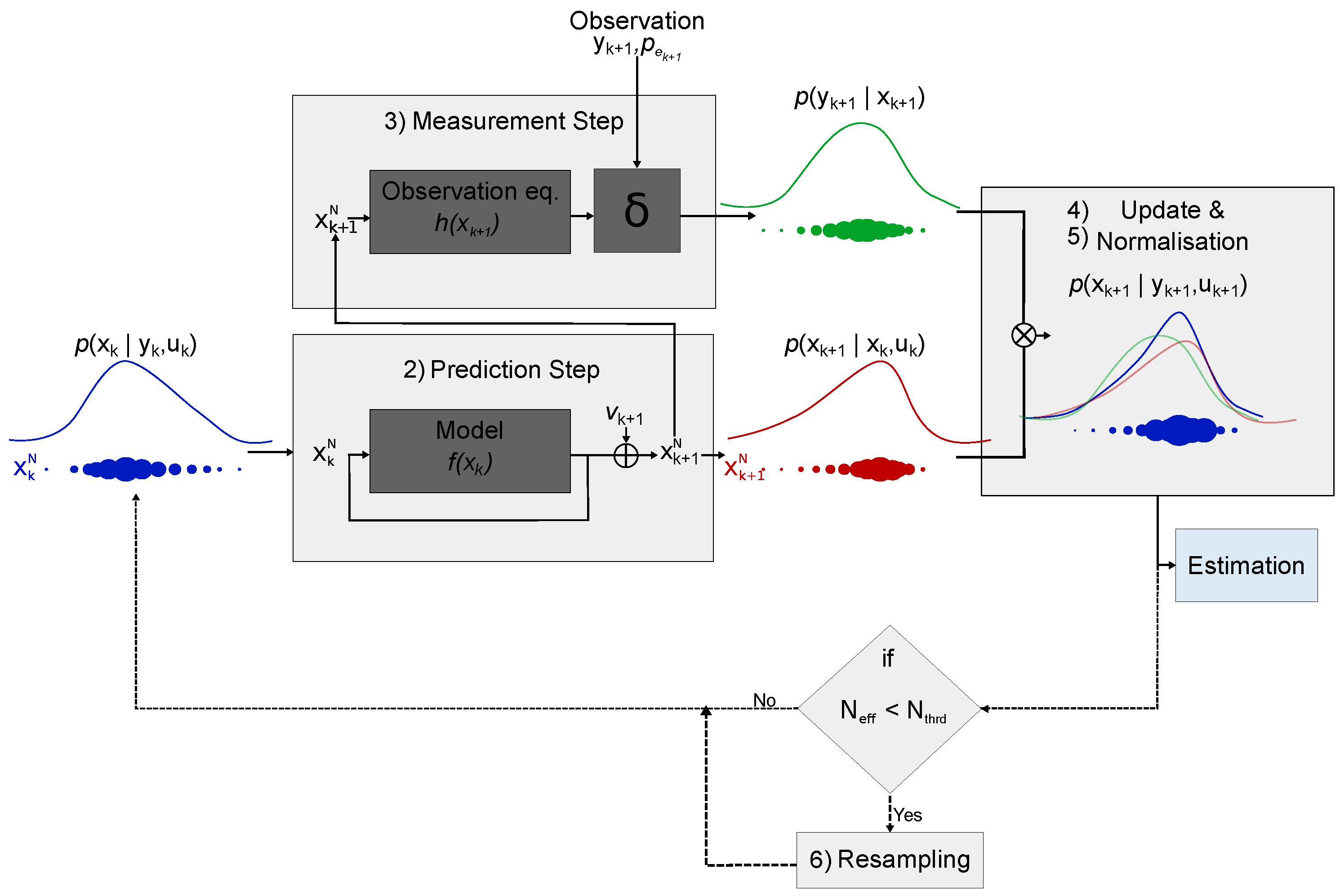
| (2) Prediction | Obtain the sample of from the transition PDF . |
| (3) Measurement step | Compute the likelihood function. . |
| (4) Update | Evaluate the importance weights from likelihood function. . |
| (5) Normalisation | Normalise the weights . |
| (6) Resampling | The effective number of particles () provides a measure of the number of particles with significant weight representing the posterior PDF. If this number is lower than a provided threshold () they are redistributed where the PDF is more likely. Reset to . |
| Year | 2008 | 2009 | 2010 | 2011 | 2013 |
|---|---|---|---|---|---|
| Number of Parcels | 11 | 13 | 13 | 9 | 8 |
| Images per Parcel | 15 | 16 | 15 | 14 | 6 |
| Images Employed | 16 | 15 | 14 | 13 | 12 | |
|---|---|---|---|---|---|---|
| asymmetric Gaussian | RMSE | 7.2 | 8.1 | 9.2 | 11.0 | 14.0 |
| MAE | 13 | 21 | 35 | 35 | 43 | |
| Double-logistic | RMSE | 7.2 | 8.1 | 9.0 | 11.0 | 14.0 |
| MAE | 13 | 21 | 37 | 39 | 43 | |
| Savistzky-Golay | RMSE | 10.2 | 11.0 | 12.4 | 14.0 | 17.7 |
| MAE | 20 | 26 | 45 | 47 | 69 | |
| Images Employed | 3 |
|---|---|
| RMSE | 8.3 |
| MAE | 24 |
© 2016 by the authors; licensee MDPI, Basel, Switzerland. This article is an open access article distributed under the terms and conditions of the Creative Commons Attribution (CC-BY) license (http://creativecommons.org/licenses/by/4.0/).
Share and Cite
De Bernardis, C.; Vicente-Guijalba, F.; Martinez-Marin, T.; Lopez-Sanchez, J.M. Particle Filter Approach for Real-Time Estimation of Crop Phenological States Using Time Series of NDVI Images. Remote Sens. 2016, 8, 610. https://0-doi-org.brum.beds.ac.uk/10.3390/rs8070610
De Bernardis C, Vicente-Guijalba F, Martinez-Marin T, Lopez-Sanchez JM. Particle Filter Approach for Real-Time Estimation of Crop Phenological States Using Time Series of NDVI Images. Remote Sensing. 2016; 8(7):610. https://0-doi-org.brum.beds.ac.uk/10.3390/rs8070610
Chicago/Turabian StyleDe Bernardis, Caleb, Fernando Vicente-Guijalba, Tomas Martinez-Marin, and Juan M. Lopez-Sanchez. 2016. "Particle Filter Approach for Real-Time Estimation of Crop Phenological States Using Time Series of NDVI Images" Remote Sensing 8, no. 7: 610. https://0-doi-org.brum.beds.ac.uk/10.3390/rs8070610