Comparison of Methods for Estimating Fractional Cover of Photosynthetic and Non-Photosynthetic Vegetation in the Otindag Sandy Land Using GF-1 Wide-Field View Data

Abstract

Photosynthetic vegetation (PV) and non-photosynthetic vegetation (NPV) are important ground cover types for desertification monitoring and land management. Hyperspectral remote sensing has been proven effective for separating NPV from bare soil, but few studies determined fractional cover of PV (f_pv) and NPV (f_npv) using multispectral information. The purpose of this study is to evaluate several spectral unmixing approaches for retrieval of f_pv and f_npv in the Otindag Sandy Land using GF-1 wide-field view (WFV) data. To deal with endmember variability, pixel-invariant (Spectral Mixture Analysis, SMA) and pixel-variable (Multi-Endmember Spectral Mixture Analysis, MESMA, and Automated Monte Carlo Unmixing Analysis, AutoMCU) endmember selection approaches were applied. Observed fractional cover data from 104 field sites were used for comparison. For f_pv, all methods show statistically significant correlations with observed data, among which AutoMCU had the highest performance (R² = 0.49, RMSE = 0.17), followed by MESMA (R² = 0.48, RMSE = 0.21), and SMA (R² = 0.47, RMSE = 0.27). For f_npv, MESMA had the lowest performance (R² = 0.11, RMSE = 0.24) because of coupling effects of the NPV and bare soil endmembers, SMA overestimates f_npv (R² = 0.41, RMSE = 0.20), but is significantly correlated with observed data, and AutoMCU provides the most accurate predictions of f_npv (R² = 0.49, RMSE = 0.09). Thus, the AutoMCU approach is proven to be more effective than SMA and MESMA, and GF-1 WFV data are capable of distinguishing NPV from bare soil in the Otindag Sandy Land.

1. Introduction

Accurate and timely information about vegetation cover is fundamental for monitoring desertification [1,2,3] and assessing the impacts of land management strategies [4] in the Otindag Sandy Land, one of the four largest sandy lands in China. This area has experienced severe desertification before 2000 [5,6], and was the focus of massive ecological engineering measures since the launch of the “Beijing and Tianjin Sandstorm Source Controlling Program” in 2001 [7]. Remote sensing offers a unique opportunity to estimate vegetation cover at large scales that might otherwise be costly, labor-intensive, and spatially discontinuous [8,9,10]. Over the past several decades, common multispectral vegetation indices, which exploit the difference between visible and near-infrared (NIR) reflectance caused by the presence of chlorophyll, such as the normalized difference vegetation index (NDVI) [11] and the enhanced vegetation index (EVI) [12], have been widely utilized for assessing vegetation cover and dynamics. However, these indices are only sensitive to the amount of photosynthetic vegetation (PV), as well as its turgidity and greenness [13].

From a functional perspective, vegetation can be categorized as photosynthetic (green leaves) and non-photosynthetic (wood, senescent material, and litter) [14]. Undoubtedly, photosynthetic vegetation is a critical component of vegetation, but it is not the only component. Non-photosynthetic vegetation (NPV) also plays a key role in carbon and nutrient uptake, fire risk and frequency, and wind and water erosion [15]. In the Otindag Sandy Land, non-photosynthetic vegetation is common due to the area’s arid climate, relatively sparse vegetation coverage, and frequent droughts. Thus, simultaneously acquiring the fractional cover of PV and NPV in the Otindag Sandy Land would provide new insights for desertification monitoring and land management.

Unlike PV, it is difficult to discriminate NPV from soils due to the similarity in reflectance between many soils and NPVs, particularly when multispectral sensors are considered [16]. The cellulose absorption index (CAI), based on hyperspectral data, has been proven to be an effective method to resolve NPV cover [17,18,19]. An alternative approach is linear unmixing of hyperspectral bands affected by cellulose and lignin to retrieve NPV cover [3] and map forest fuel [20], and to monitor degradation and desertification [21]. However, hyperspectral images are difficult to acquire and cannot meet the demand of NPV cover retrieval at large scales. To date, there are few methods for retrieval of NPV dynamics from multispectral imagery. In the past, numerous studies focused on developing a new multispectral spectral index sensitive to NPV such as the normalized difference senescent vegetation index (NDSVI) [22], the soil adjusted total vegetation index (SATVI) [23], a ratio of moderate resolution imaging spectrometer (MODIS) bands 7 and 6 [14], and the dead fuel index (DFI) [24]. Although NPV estimation results using these spectral indices in different environments showed good agreement with field data, this approach is area-specific, and not well validated in other environments.

Spectral mixture analysis (SMA) provides another promising method for retrieving NPV cover from multispectral imagery [15,25]. A crucial factor affecting the performance of SMA for NPV cover retrieval is the knowledge of the soil background spectrum for each pixel. In order to resolve endmember spectral variability, multiple endmember SMA (MESMA) and relative spectral mixture analysis (RSMA) have been utilized for PV and NPV cover estimation in an agricultural area [26]. However, the choice of the appropriate SMA techniques and endmember spectra may still cause uncertainties, even for simple vegetation structure. The selection of appropriate endmembers, which are usually selected either from the image data [21] or from spectral libraries acquired from field investigations [25], is also critical to the accurate estimation of fractional cover. Each approach has distinct merits and drawbacks. Image-based endmembers are ideal for their consistency in data to be analyzed. However, determination of image endmembers often requires the existence of pure pixels, which are rarely available at 10–30 m spatial scale, especially in arid and semi-arid regions. Field-measured endmembers can be readily collected and their quality can be easily controlled. However, there are potential problems related to the generality and scalability of endmembers. In addition, most SMA techniques for PV and NPV cover estimation were applied to multispectral sensors with short-wave infrared (SWIR) bands (e.g., Landsat TM, and MODIS), and there is limited literature reporting PV and NPV cover estimation using visible and NIR bands only. The GF-1 wide field view (WFV) cameras, which only include four bands in the visible and NIR regions, are highly valuable data sources for dynamic monitoring of vegetation cover at large scales, due to their high spatial resolution (16 m), wide coverage (800 km), and high revisit frequency (2–3 days).

Therefore, the objective of this study is to examine, for the first time, the performance of different SMA techniques for simultaneously estimating the fractional cover of PV and NPV with GF-1 WFV data (only visible and NIR bands), and to compare the results to observed fractional cover measurements in the Otindag Sandy Land.

2. Materials and Methods

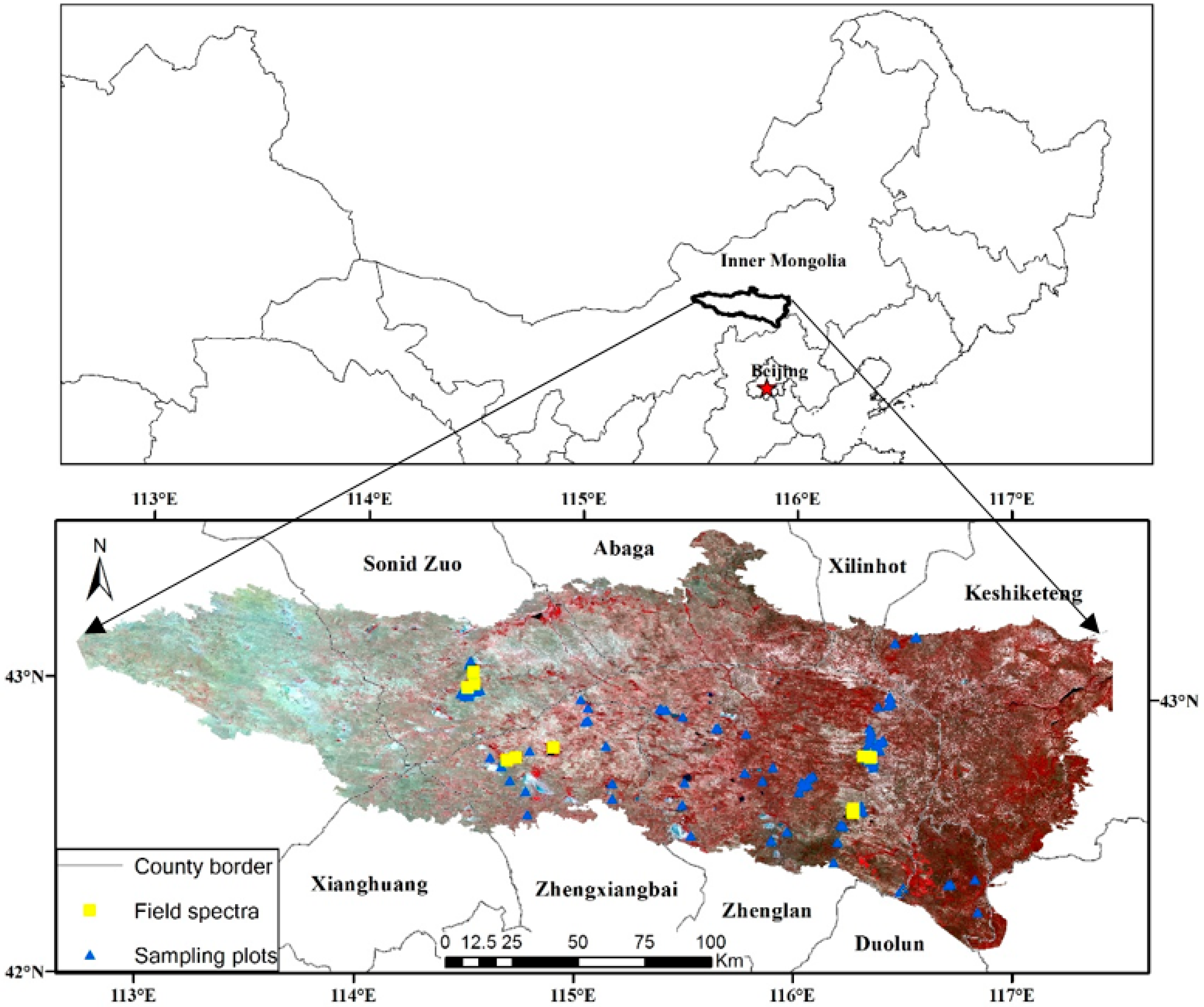
2.1. Study Area

The Otindag Sandy Land is located in central-eastern Inner Mongolia, north of Beijing (Figure 1). The area is about 360 km in length from east to west and 30–100 km in width, with an elevation between 1100 m and 1400 m above sea level, decreasing from southeast to northwest. It is characterized by a temperate continental semi-arid climate with strong wind and less precipitation in winter and spring. Annual average precipitation, mainly occurring in summer and fall with some interannual fluctuation, is 350–400 mm in the southeastern part and below 200 mm in the northwestern part. The major soil type is sandy soil formed by Aeolian processes. The vegetation is characterized by open forest steppe and meadow prairie in the east, semi-arid grassland in the central part, and desert prairie in the west (Figure 2). Because of desertification, most grasslands have experienced different degrees of shrub encroachment. Therefore, the vegetation structure in the Otindag Sandy Land is highly heterogeneous. Due to the scarcity and intra-annual variation of precipitation, NPV accounts for a high percentage of the total vegetation and varies both seasonally and inter-annually.

2.2. Data Used in this Study

2.2.1. Remote Sensing Data

The GF-1 satellite operates in a sun-synchronous orbit at an altitude of 645 km and carries four wide-field view (WFV) cameras. In this study, five scenes of GF-1 WFV with four bands (blue, green, red, and NIR), provided by China Center for Resource Satellite Data and Application (CRESDA, http://www.cresda.com/), were utilized to cover the entire Otindag Sandy Land (

Table 1. Details of the GF-1 wide-field view (WFV) data used and its properties.

Sensor	Acquisition Date	Spectral Bands
WFV3	31 July 2014	450–520 nm (Blue)
WFV3	31 July 2014	520–590 nm (Green)
WFV4	31 July 2014	630–690 nm (Red)
WFV4	31 July 2014	770–890 nm
WFV2	4 August 2014	(Near infrared)

).

GF-1 WFV preprocessing is crucial for any quantitative application. First, the digital number (DN) value was converted to radiance using calibration coefficients obtained from the CRESDA. Then, radiance was transformed to surface reflectance using the Fast Line-of-sight Atmospheric Analysis of Spectral Hypercubes (FLAASH) algorithm provided with the Environment for Visualizing Images Software (ENVI 5.0). Finally, eight Landsat-8 Operational Land Imager (OLI) datasets provided by the United States Geological Survey (USGS), which have been shown to be geometrically consistent with the field GPS values, were selected as the base map for geometric correction. The geometric correction was conducted in ENVI 5.0, and the resultant geometric co-registration error is less than one pixel of the Landsat-8 OLI panchromatic data (15 m).

2.2.2. Field Spectroscopy

Recognizing the multitude of highly variable PV, NPV, and bare soils in the Otindag Sandy Land, their spectral properties were thoroughly investigated in order to acquire the most generalizable endmember dataset (Figure 1). Spectra were collected with an Analytical Spectral Devices (ASD) full-range (350–2500 nm) Fieldspec^® 4 spectroradiometer with a 25° sensor foreoptic. All measurements were collected within two hours of local solar noon on clear sky days. The sensor was held 1 m above the top of the PV and NPV canopy or bare soil surface in a vertical downward position. Prior to each measurement, the spectroradiometer was calibrated to a Spectralon^® white reference target.

Field spectra were collected during two periods. The first measurement was conducted on 27 and 31 July 2014, representative of maximum PV existence, quasi-synchronous with the GF-1 data acquisition time. Twenty-nine PV spectra, 14 NPV spectra, and 12 bare soil spectra were recorded across the whole region. In order to acquire additional NPV spectra, a second measurement was conducted on 4 and 5 November 2014, representative of maximum NPV existence. Fourteen NPV spectra and three bare soil spectra were acquired. Finally, an endmember library, consisting of 29 PV, 28 NPV, and 15 bare soil spectra, was established. Based on the spectral response function of the GF-1 WFV sensor, the field spectra were resampled to the GF-1 WFV bands (Equation (1)), where $R_i$ is the simulated GF-1 WFV reflectance, $f_i\left(\lambda \right)$ is the spectral response function at $\lambda$ wavelength of GF-1 WFV band ith, $r\left(\lambda \right)$ is the field observed reflectance at $\lambda$ wavelength, and ${\lambda }_{min} and {\lambda }_{max}$ represents the band width of GF-1 WFV band ith.

$$R_i=\frac{{{\displaystyle \int }}_{{\lambda }_{min}}^{{\lambda }_{max}}{f}_i\left(\lambda \right)r\left(\lambda \right)d\lambda }{{{\displaystyle \int }}_{{\lambda }_{min}}^{{\lambda }_{max}}{f}_i\left(\lambda \right)d\lambda }$$

(1)

2.2.3. Fractional Ground Cover Data

Fractional ground cover data were collected in late July and early August, the season of maximum green vegetation cover in 2014. Based on a stratified random design and accessibility, 104 sites were selected (Figure 1), and one 32 m × 32 m plot was set up in each site. For sampling, two transects coinciding with the diagonal lines across the plot were applied, where vegetation cover in the three categories (non-woody ground cover, woody less than 2 m high, and woody greater than 2 m in height) is recorded. Using a tape laid on the ground, the surveyor recorded the presence of PV, NPV, and bare soil at 1-m intervals using a laser pointer. Non-woody vegetation was observed by looking downward, while woody vegetation was observed by looking upward or downwards where vegetation was less than the observer’s height. Total cover fractions per category were calculated by dividing the number of counts of a particular cover type by the total number of counts (90). For each plot, an exposed planar fractional cover was calculated by merging all presented categories, based on the approach proposed by Muir et al. (2011) [27]. The coordinates of the cross point of the two transects were recorded by a global position system device (Trimble GeoXT 2800–3000) with a positioning accuracy of approximately ±3 m to match the GF-1 WFV data.

2.3. Methods

2.3.1. Spectral Mixture Analysis

In SMA, the reflectance of a pixel is assumed to be a linear combination of the reflectance of the spectra of the endmembers, weighted by their fractional cover. Endmembers are fundamental physical components that themselves are not mixtures of other components. SMA assumes that the endmembers are spatially and temporally invariant. In this study, the average spectra of PV, NPV, and bare soil were utilized as the endmember spectra.

2.3.2. Multiple Endmember SMA

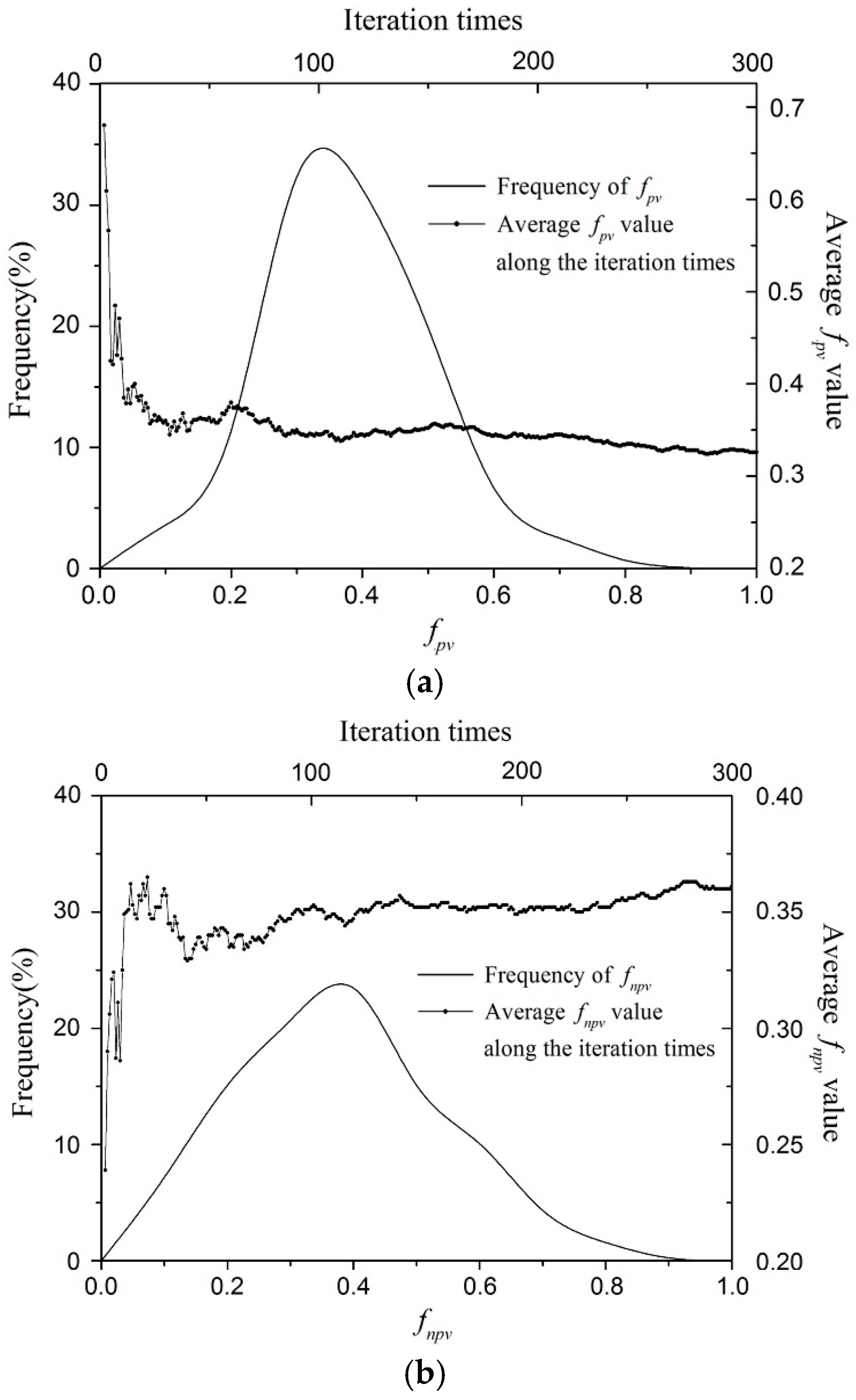
Multiple Endmember SMA was developed to handle the endmember variability problem through the utilization of iterative mixture analysis cycles [28]. In MESMA, endmembers are allowed to vary on a per-pixel basis. When all endmember combinations are calculated, the best-fit model is determined for each pixel. One criterion most often used in MESMA is the lowest Root Mean Square Error (RMSE) of spectral fit [28]. In this study, models were calculated by utilizing all possible combinations among 29 PV spectra, 27 NPV spectra, and 15 bare soil spectra resulting in 11,745 total models.

2.3.3. AutoMCU

Another approach dealing with endmember variability, the Automatically Monte Carlo spectral Unmixing model (AutoMCU), was proposed by Asner and Lobell [29], in which, a large number of endmember combinations for each pixel is calculated by randomly selecting spectral data from a spectral library. Studies [25,29] have shown that the fractional cover of different endmembers is distributed normally when the number of endmember combinations is sufficient. Thus, the average value of the fractional cover for different models was used as the final fractional cover of each pixel. We set up an initial value of 300 iterations, followed by a determination of the appropriate times through the analysis of the average fractional cover dynamic. If the average fractional cover does not vary with the increasing unmixing iterations, this time would be considered as the appropriate time.

2.3.4. Unmixing Strategy

The three approaches are different with regard to endmember selection. The Fully Constrained Least Square (FCLS) algorithm was applied for calculating $f_k$ at each time [30]. Using FCLS, two important constraints on $f_k$ (the fraction sum-to-one constraint (ASC) ${\displaystyle \sum }_{k=1}^n{f}_k=1$ and the fraction nonnegativity constraint (ANC) $f_k\ge 0$) could be resolved simultaneously.

According to the linear unmixing model, the spectral signature of a pixel vector $r$ can be represented by a linear regression model of $\mathsf{\rho }$ as follows:

$$r =\mathsf{\rho }f+\mathsf{\epsilon }$$

(2)

In order to account for ASC, we included ASC in the signature matrix $\mathsf{\rho }$ by introducing a new signature matrix, denoted by M and defined as:

$$M=\left[\begin{array}{c}\mathbf{\delta }\mathbf{\rho }\\ 1^T\end{array}\right]$$

(3)

with $1=\underset{n}{\underbrace{{\left(1,1,\dots ,1\right)}^T}},$and a vector $R=\left[\begin{array}{c}\delta r\\ 1\end{array}\right]$, where $\mathsf{\delta }$ is a weight for deciding the degree of ASC; the smaller the $\mathsf{\delta }$ value, the closer the sum to one. A value of 1 was applied in this study. Combining Equations (2) and (3), the following equation is obtained:

$$R=Mf+\epsilon$$

(4)

The nonnegatively constrained least squares (NCLS) imposes the nonnegativity constraint (ANC) on the abundance vector while estimating fractional cover. The estimation of abundances subject to nonnegative constraints is difficult to implement since it results in a set of inequalities and can only be solved by numerical methods. The iteration algorithm proposed by Chang and Heinz [31] was adopted by introducing a Lagrange multiplier vector (λ). The algorithms for FCLS, SMA, MESMS, and AutoMCU were transformed into IDL (Interactive Data Language) routines.

2.3.5. Comparison with Observed Data

To compare the performance of different SMA techniques on PV/NPV fractional cover estimation, two metrics were calculated against observed data, the RMSE and coefficient of determination (R²) of linear regression:

$$\mathrm{RMSE}=\sqrt{{\displaystyle \sum }_{i=1}^n{\left(x_i-y_i\right)}^2/n}$$

(5)

$$R^2=\frac{{{\displaystyle \sum }}_{i=1}^n\left(x_i-\overline{x}\right){\left(y_i-\overline{y}\right)}^2}{{{\displaystyle \sum }}_{i=1}^n{\left(x_i-\overline{x}\right)}^2{{\displaystyle \sum }}_{i=1}^n{\left(y_i-\overline{y}\right)}^2}$$

(6)

where n is the number of fields,$x_i$ is the estimated fractional cover of field i, $y_i$is the measured fractional cover of field i, $\overline{x}$ is the average value of the estimated fractional cover, and $\overline{y}$ is the average value of the measured fractional cover.

3. Results

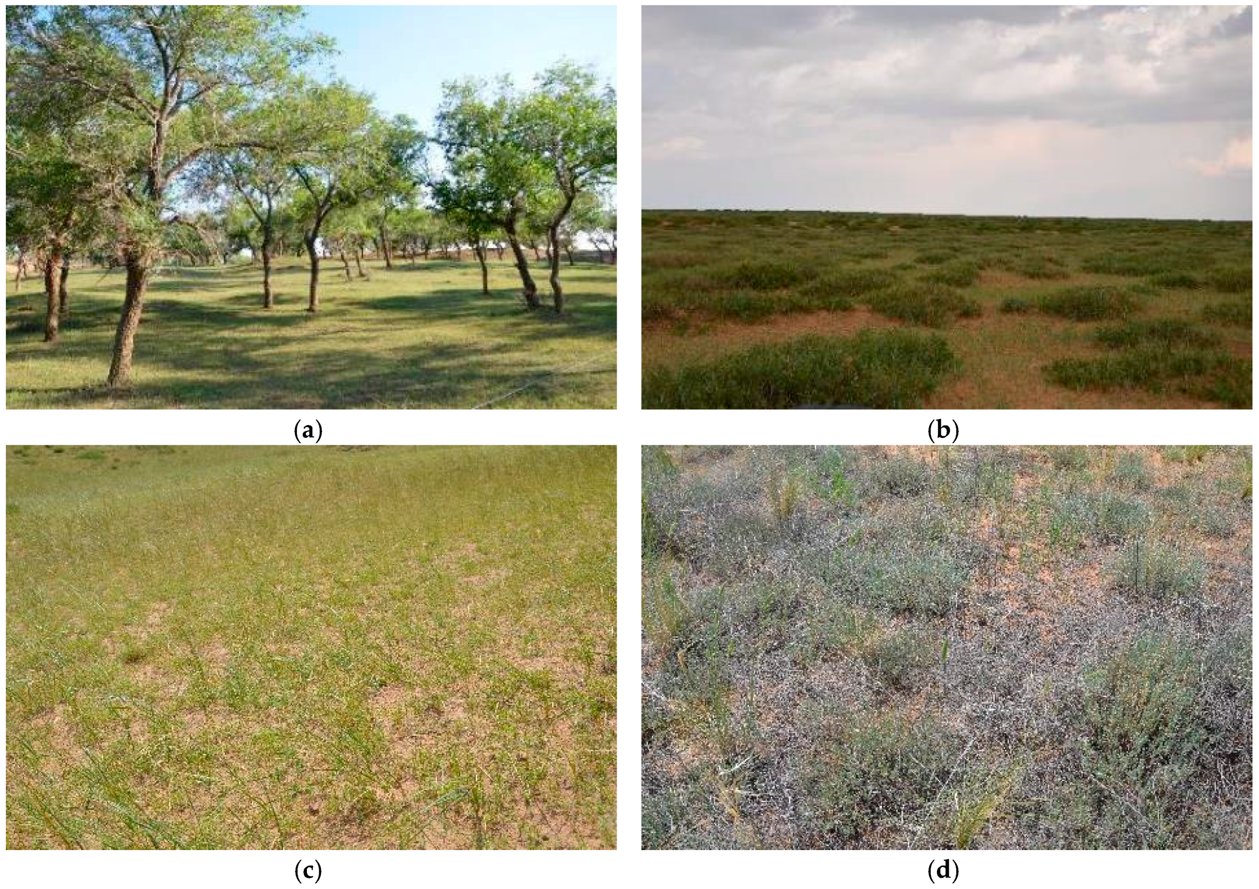
3.1. Field f_pv f_npv, and f_soil Measurements

Totally, 104 sample plots were investigated, 12 in open woodland, 40 in grassland encroached by shrub and 52 in grassland, respectively. Field observed f_pv, f_npv, and f_soil followed the expected temporal and structural patterns (

Table 2. Characteristics of sample plots. Values shown for f_pv, f_npv, and f_soil are average ± standard deviations.

Sample Plots Type	Numbers	fpv	fnpv	fsoil
Open woodland	12	0.44 ± 0.20	0.24 ± 0.10	0.30 ± 0.22
Grassland encroached by shrub	40	0.52 ± 0.15	0.14 ± 0.12	0.32 ± 0.17
Grassland	52	0.57 ± 0.23	0.14 ± 0.10	0.29 ± 0.24
Total	104

). Because the acquiring time corresponds to the maximum vegetation growing season, fields were dominated by green vegetation resulting in high f_pv. Even so, NPV takes an important proportion of sample plots, especially in open woodland (average f_npv reaches 24%). Compared to grassland, the open woodland was characterized by higher f_npv and lower f_pv, while no obvious difference was observed for f_soil.

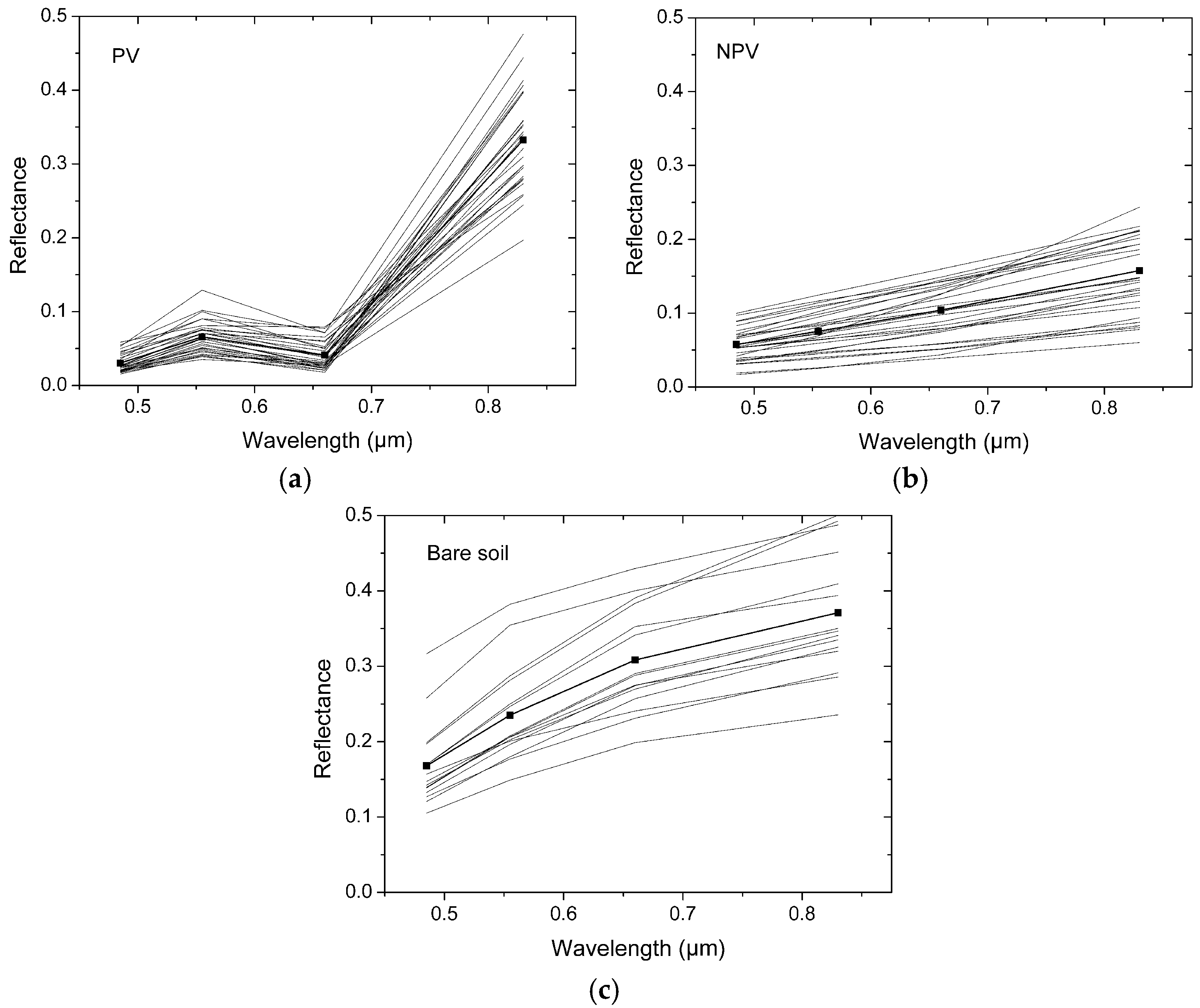
3.2. Endmember Library and Variability

The endmember library for the Otindag Sandy Land, divided into PV, NPV, and bare soil categories and consistent with GF-1 WFV data, was established (Figure 3). It is obvious that the PV spectra are easily distinguishable from NPV and bare soil spectra. However, the NPV and bare soil spectra are similar, both exhibiting a monotonous increasing tendency, which makes separation more difficult. Even so, there are some differences between NPV and bare soil spectra. First, bare soil spectra show a significantly higher reflectance than the NPV spectra, mainly due to extensive bright sandy substrate. Second, a bow-shaped protuberance, which was first recognized by Gao et al. [32], exists from the blue to the red bands in the bare soil spectra, while it is absent in the NPV spectra. These spectral characteristics of NPV and bare soil provide new opportunities for the discrimination of NPV from bare soil in the Otindag Sandy Land. With regard to intra-variability of the three endmember categories, the PV and NPV spectra are relatively concentrated, while the bare soil spectra vary greatly. Therefore, the bare soil endmember selection will have a greater influence on fractional cover estimation, especially on the fractional cover of NPV. In any case, the choice of optimal endmember combinations is crucial for the spectral unmixing process. While MESMA will try all combinations of PV, NPV, and bare soil endmembers, AutoMCU will utilize as many combinations as necessary through random selection. For SMA, the average spectra of three endmember categories were employed as invariant PV, NPV, and bare soil spectra for spectral unmixing.

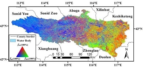
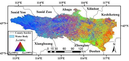
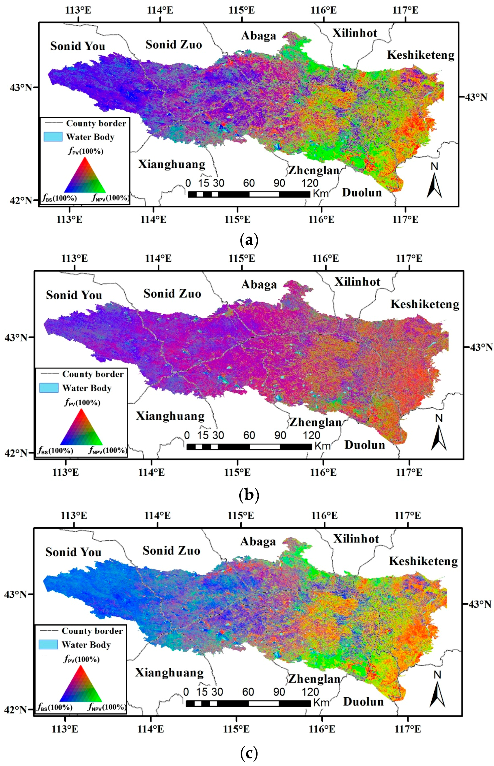
3.3. Fractional Cover Estimation and Validation

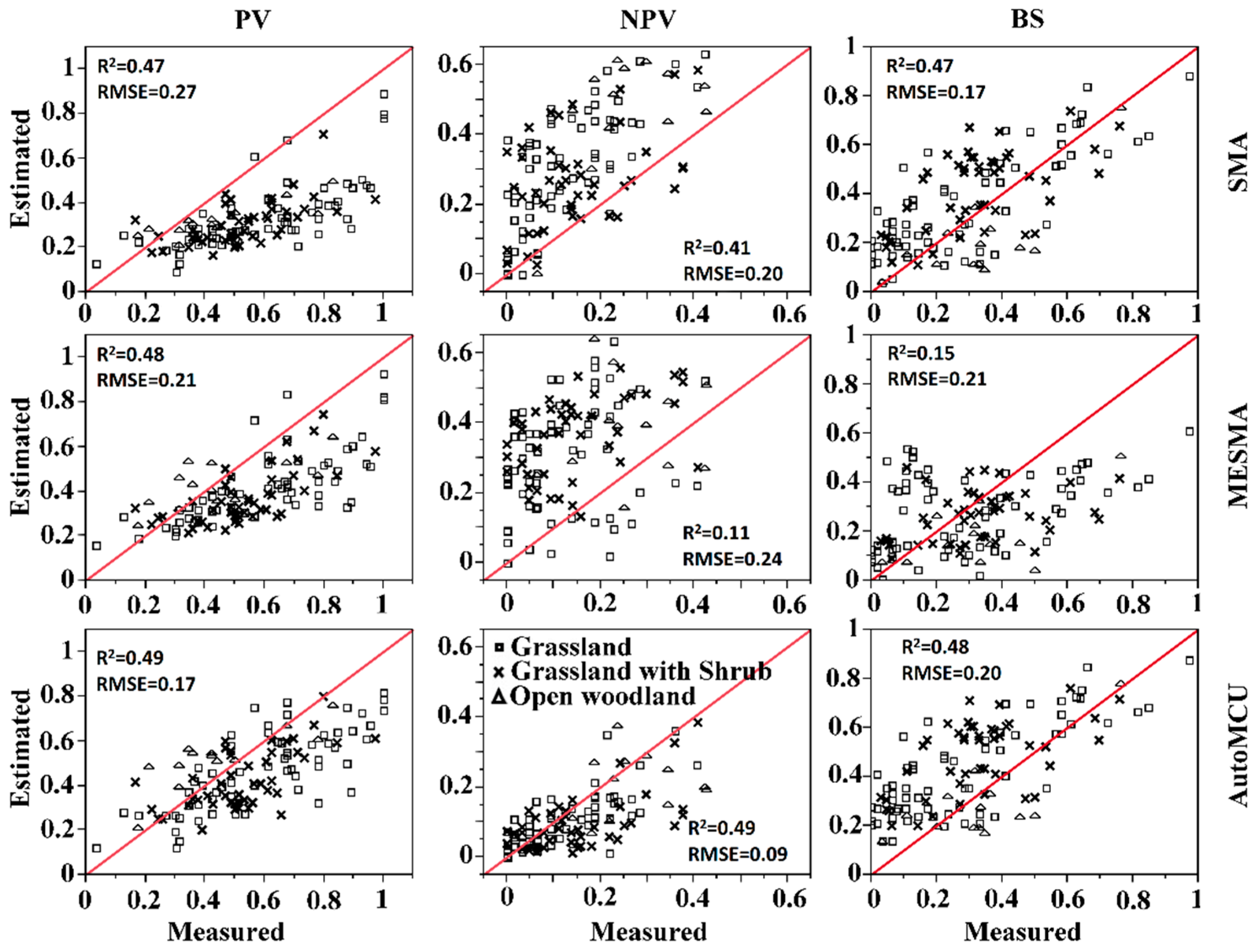
3.3.1. SMA

Choosing the average PV, NPV, and bare soil spectra as endmembers, f_pv, f_npv, and f_soil in the Otindag Sandy Land were estimated using the FCLS algorithm. The RMSE of SMA for the samples ranges from 1.24% to 19.91%, with an average RMSE value of 3.76%. The spatial distribution of f_pv and f_npv is shown in Figure 4a. Overall, the spatial distribution characteristics are consistent with prior field investigations. From east to west, the fractional cover of both PV and NPV shows an obvious decreasing tendency, coincident with decreasing precipitation. The high f_pv, mainly located in the eastern part of the Otindag Sandy Land, corresponds to forest, farmland, and wetland. The high f_npv, was mainly found in the grassland along the southern and northern edge of the eastern Otindag Sandy Land, and the high f_soil mainly correspond to desert steppe and active sand dunes, respectively.

Based on the 104 field samples, the validation results of SMA-based f_pv and f_npv are shown in Figure 5, and their statistical data are summarized in

Table 3. Regression analysis and validation of remote sensing results against observed data.

Unmixing Approach	PV					NPV					BS
	R2	RMSET	RMSEOW	RMSEGS	RMSEG	R2	RMSET	RMSEOW	RMSEGS	RMSEG	R2	RMSET	RMSEOW	RMSEGS	RMSEG
AutoMCU	0.49 *	0.17	0.14	0.16	0.19	0.49 *	0.09	0.13	0.10	0.07	0.48 *	0.20	0.13	0.22	0.20
MESMA	0.48 *	0.21	0.15	0.20	0.23	0.11	0.24	0.21	0.25	0.25	0.15	0.21	0.21	0.18	0.23
SMA	0.47 *	0.27	0.19	0.25	0.29	0.41*	0.20	0.25	0.18	0.21	0.47 *	0.17	0.17	0.18	0.16

BS stands for bare soil. RMSE_T stands for total RMSE, RMSE_OW stands for the RMSE of open woodland samples, RMSE_GS stands for the RMSE of grassland with shrub samples, RMSE_G stands for the RMSE of pure grassland samples. * p < 0.0001.

. It can be seen that the SMA-based f_pv and f_npv are highly correlated with observed data, with R² values of 0.47 and 0.41, respectively. However, there is an obvious underestimation of f_pv (RMSE = 0.27), and an obvious overestimation of f_npv (RMSE = 0.20). The high correlation demonstrates that PV and NPV can be distinguished by SMA using GF-1 WFV data, but the absolute error suggests that using the average spectra of the PV, NPV, and bare soil endmember library as the invariant endmember is problematic.

3.3.2. MESMA

The spatial distribution of f_pv, f_npv and f_soil is shown in Figure 4b. The overall spatial pattern is consistent with the SMA-based results, but with obvious difference of f_pv, f_npv in the east Otindag Sandy Land. The minimal RMSE was selected as the criterion to choose the appropriate endmember from the endmember library. The RMSEs of MESMA for the sample plots range from 0% to 8.46%, with an average RMSE value of 0.53%, significantly lower than that of the SMA (3.76%), indicating that MESMA fits the GF-1 WFV data better than SMA.

In Figure 4, we can see that MESMA-based f_pv correlate with observed f_pv well (with R² of 0.48), but with the obvious underestimation of f_pv (RMSE = 0.21). However, the accuracy of MESMA-based f_npv and f_soil are poor, with a weak relationship with observed data (with R² of 0.11 and 0.15, respectively). Therefore, MESMA performs better for f_pv, because the PV endmember is clearly different from the NPV and bare soil endmembers, but would lead to confusion with regard to f_npv and f_soil because of the similarities of the NPV and bare soil endmember spectra.

3.3.3. AutoMCU

The AutoMCU was firstly utilized for the GF-1 WFV pixels corresponding to the 104 field samples with 300 iterations. The f_pv and f_npv distribution and their average values along unmixing times obey the same change rules, one of which is illustrated in Figure 6. The f_pv and f_npv values are highly variable during the first 50 iterations, indicating that endmember selection evidently influences f_pv and f_npv estimation results. When the number of iterations exceeds 150, the mean f_pv and f_npv values are essentially stable. In addition, the f_pv and f_npv distributions follow Gaussian distribution, indicating that their expected (average) values represent the true values. Therefore, 150 iterations were used for unmixing of the entire GF-1 WFV dataset by AutoMCU.

The validation results of AutoMCU-based f_pv, f_npv, and f_soil show that AutoMCU performs well for f_pv and f_npv. The R² of the regression of f_pv and f_npv on observed data is 0.49, indicating a significant correlation with observed data. The RMSEs for the f_pv and f_npv estimation are 0.17 and 0.09, respectively.

3.3.4. Comparisons of Different Methods

The computation efficiency of the three approaches varies widely, depending on the total unmixing times for each pixel. SMA is the fastest (only one time), followed by AutoMCU (150 times), and MESMA is the slowest since all endmember combinations would be used (11,745 times).

The accuracy of these approaches is also obviously different (Table 3). The accuracy of MESMA-based f_pv was improved compared to SMA (increase in R² from 0.47 to 0.48, and decrease in RMSE from 0.27 to 0.21), and the underestimation of f_pv in SMA was alleviated slightly. However, the accuracy of MESMA-based f_npv deteriorates significantly, with a weak relationship with observed data (R² = 0.11) and an increase in the RMSE from 0.22 to 0.24. In addition, the MESMA-based f_npv was significantly overestimated, similar to SMA. Therefore, MESMA performs better for estimating f_pv, but would lead to serious mistakes for f_npv and f_soil. Therefore, AutoMCU is an effective approach for f_pv and f_npv estimation in the Otindag Sandy Land because it performs better than SMA and MESMA.

The accuracies for f_pv and f_npv estimation are different for different land cover types. For example, in f_pv estimation with the AutoMCU approach, grassland has the highest RMSE (0.19), followed by grassland encroached by shrub (RMSE = 0.16) and open woodland (RMSE = 0.14). However, the opposite tendency appears in f_npv estimation. Open woodland has the highest RMSE (0.13), followed by grassland encroached by shrub (RMSE = 0.10), and grassland (RMSE = 0.07). Differences in accuracy were consistent with differences in average f_pv and f_npv values of sample plots in different land cover types (Table 3).

4. Discussion

4.1. Separability of NPV and Bare Soil in SMA

The separation of PV from others is not difficult, and it is widely used with VIS-NIR bands [11,12,13]. Therefore, the method of distinguishing NPV and Bare soil is critical in this study. Unlike other regions, there are two differences between bare soil and NPV spectra in Otindag Sandy Land. First and foremost, the absolute reflectance of bare soil is obviously higher than that of NPV. In addition, a bow-shaped protuberance exists in bare soil when observed from the spectral library, but it is absent in NPV. However, this characteristic is not sufficiently significant because of the coarse spectral resolution. Therefore, the higher reflectance of bare soil relative to NPV due to the extensive sandy substrate is an important prerequisite for separating NPV from bare soil in the Otindag Sandy Land, indicating that this approach cannot be used in regions with a large percentage of dark colored bare soil.

For a given pixel, the key point for successfully estimating f_npv and f_soil using the GF-1 WFV data is the determination of appropriate endmembers—especially the bare soil endmember, which shows large intra-variability when compared to NPV spectral libraries—and not the absolute difference of reflectance of NPV and bare soil. Thus, identifying the most appropriate NPV and bare soil endmember for unmixing is critical for retrieving ground cover accurately.

4.2. Effects of Endmember Variability

In this study, three unmixing approaches for determining the appropriate endmember combinations, SMA, MESMA, and AutoMCU, were compared to estimate f_pv and f_npv in the Otindag Sandy Land with GF-1 WFV data. Table 2 shows that all SMA-based fractions are highly correlated with observed data, but that f_pv is clearly underestimated, while f_npv is overestimated; only f_soil shows no directional bias. Thus, the use of the average spectra of PV and NPV as invariant endmembers is not appropriate, but identifying the most representative PV and NPV endmember spectra is extremely difficult.

In order to resolve this problem, MESMA was developed to explore “optimal” pixel-varied specific endmember combinations by setting up a selection criterion (e.g., the lowest RMSE), which has been proven to be effective for estimating f_pv and f_npv using Landsat [33], MODIS [34] and, Geoeye [35] data. However, MESMA was shown to be incapable for f_npv estimation with GF-1 WFV data in the Otindag Sandy Land, because it would lead to serious confusion between NPV and bare soil, with R² values of 0.11 and 0.15, and RMSEs of 0.24 and 0.21, respectively. The endmembers most frequently utilized in MESMA are shown in Figure 7. Three PV (including mean spectra), seven NPV, and four bare soil endmembers were utilized most frequently, accounting for 70%, 68%, and 93%, respectively. From the spectral curve, we can see that the bare soil endmember spectra differ more widely than those for PV and NPV. Thus, the selection of the bare soil endmember will have a significant effect on the unmixing results. For example, the use of the bare soil endmember with obviously higher reflectance would lead to a significant underestimation of f_soil. Therefore, the appropriate bare soil endmember determination would be essential for estimating f_npv and f_soil accurately. Since the spectral similarity between NPV and bare soil, the actual NPV and bare soil endmember combinations could be replaced by another combinations in MESMA in order to minimize the RMSE of spectral fit. This finding is consistent with Okin et al. [26], who found that MESMA did not improve f_soil estimates, because the similarity between soil and NPV spectra can actually lead to errors in MESMA as some bare soil/NPV combinations may be mistaken as combinations of other bare soil/NPV [36]. Therefore, it cannot be assumed that MESMA always leads to better f_npv and f_soil estimates.

The AutoMCU method, which randomly selects endmembers from the spectral library to unmix the image over several iterations, rather than doing an exhaustive search, has successfully been applied to arid and semi-arid rangeland [25,37,38,39] for f_pv and f_npv estimation. Like in previous studies, the AutoMCU is shown to be effective in semi-arid sandy lands. In addition to improving computational efficiency, AutoMCU is able to explicitly quantify the proportion indeterminacy [40]. It is worth noting that the AutoMCU was originally designed for hyperspectral sensors [25], and that only few studies applied it to multispectral sensors, mainly Landsat [37,41], but with a lack of quantitative validation of f_pv and f_npv. The distinguishing feature of this study is that we were able to show that GF-1 WFV data, lacking the short-wave infrared bands, are capable of distinguishing NPV from bare soil in the Otindag Sandy Land.

Differences in the spatial distribution of f_pv and f_npv are shown in Figure 8. Compared to SMA, AutoMCU-based f_pv became higher (up to 10%) in east Otindag Sandy Land, except for cropland and wetland with the highest green vegetation cover, and decreased (up to 16%) in the entire west Otindag Sandy Land, corresponding to desert steppe; AutoMCU-based f_npv decreased for most vegetated areas (up to 20%), resolving the overestimation problem of f_npv in the SMA (Figure 5). However, there are extensive regions with increasing f_npv (up to 10%), which were verified to correspond to regions with a bright background of sandy soil. More importantly, these increases do not lead to more serious overestimation. Thus, f_npv estimation accuracy was improved effectively. Compared to the MESMA, AutoMCU-based f_pv and f_npv changed dramatically, because MESMA led to a serious confusion between NPV and bare soil. f_pv increased for vegetated areas and decreased for sandy lands, which alleviated the underestimation problem of f_pv in MESMA. f_npv decreased significantly for salt marshes in west regions, which was misclassified as NPV in MESMA.

4.3. Cross-Multispectral Sensor Comparison

Based on GF-1 WFV data, the unmixing results indicate that the f_pv estimations are relatively stable, regardless of the method used. Estimated f_pv is significantly correlated with field observed f_pv (p < 0.0001), with R² values ranging from 0.47 to 0.49. In addition, the obvious underestimation problem gradually improved from SMA to MESMA and AutoMCU, which shows that the per-pixel variable endmember combinations will increase the accuracy of the f_pv estimation. However, the f_npv estimations are highly variable: the SMA- and AutoMCU-based f_npv estimates are significantly correlated with field observed f_npv, with R² values of 0.41 and 0.49, respectively, but, the correlation between MESMA-based f_npv and in situ f_npv is poor (R² = 0.11).

In general, the AutoMCU approach results in an optimal estimation of f_pv and f_npv. Here, f_npv is estimated most accurately, with an RMSE of 0.09 (R² = 0.49), while f_pv is estimated less accurately, with an RMSE of 0.17 (R² = 0.49), and f_soil shows the worst estimation results, with an RMSE of 0.20 (R² = 0.48). An important aspect of this study is the field verification. Few studies compare f_pv and f_npv from multispectral remote sensing imagery with field measurements.

Table 4. Comparison of multispectral remote sensing-based f_pv and f_npv estimates.

#	Reference	Source Data	Study Region and Area	Study Period	Approach	Validation Points	RMSE of fpv	RMSE of fnpv
1	Guerschman et al. (2012) [42]	MODIS NDVI and the ratio of MODIS bands 7 and 6	Australia; ~7.7 × 106 km2	2000–2010	SMA	567	14.7%	20.5%
2	Okin et al. (2013) [26]	MODIS	Australia; ~150 km2	April, July and October 2010	SMA, MESMA	27	7%–23%	12%–29%
3	Guerschman et al. (2015) [43]	Landsat and MODIS	Australia; ~7.7 × 106 km2	2000–2013	SMA	1171	11.2%–11.9%	16.2%–17.4%
4	Current study	GF-1 WFV	Otindag Sandy Land of North China; ~3.0 × 104 km2	Peak growing season, 2014	SMA, MESMA and AutoMCU	104	17%–27%	9%–24%

[26,42,43] lists recently published results for f_pv and f_npv estimation based on different multispectral sensors. Since source data, study region, and study period differ, the comparison to our study is limited. For f_pv estimation, this study shows lower accuracy, with the lowest RMSE acquired by AutoMCU of 17%, while the RMSE numbers of previous studies range from 7% to 14.7%. However, this study demonstrates improved f_npv estimation: the lowest RMSE acquired by AutoMCU is 9%, compared to the previous studies’ 12%–20.5%. An important difference is that the accuracy for f_npv estimation is higher than that for f_pv estimation, which might partly be caused by the lower field observed f_npv coverage (≤45%) during the peak growing season in our study area, while field observed f_npv values ranged from 0% to 100% when multi-temporal data were considered. Our main goal was to validate the ability of the four-band GF-1 WFV (not including any SWIR bands) to distinguish PV and NPV from bare soil. Based on f_pv and f_npv estimation accuracy comparisons, we conclude that both f_pv and f_npv can be determined with modest accuracy using GF-1 WFV data with the AutoMCU approach.

4.4. Uncertainties, and Sources of Error

The field patch was usually larger than 2 × 2 GF-1 WFV pixels with a homogeneous vegetation growth status. Therefore, the plot scale (32 m) may represent the scale of a GF-1 WFV pixel (16 m), and the geometric co-registration error from field measurements to GF-1 WFV data was effectively reduced.

Time differences may occur between field observations and the time of GF-1 WFV data acquisition. This effect was minimized because the time difference did not exceed one week. We identified some particular cases of large PV underestimation for grassland sites when the observation was made before grass cutting, but the GF-1 WFV image was acquired after grass cutting. However, grass cutting in early August is relatively rare, and therefore, it has no significant effects on the accuracy assessment.

The f_pv and f_npv estimation errors could be partially related to errors in the field measurements. Sampling procedure along the diagonal lines has been widely acknowledged to be effective for ground cover measurement of sample plots, wherein vegetation is not distributed in parallel rows [44,45]. In particular, field surveyors were well trained and measurements of each transect for the first 20 sample plots were cross-validated to guarantee reliability of the field reference data. However, there were some errors caused by the observer’s bias. It is most difficult to acquire consistent field data for NPV and estimates can vary greatly between observers. This can result in the confusion between PV and NPV.

5. Conclusions

We investigated the use of different spectral unmixing approaches (SMA, MESMA, and AutoMCU) for simultaneously estimating f_pv and f_npv based on GF-1 WFV data without any SWIR bands. The unmixing results were evaluated against observed data collected concurrently with image acquisition. The main findings are:

(1)

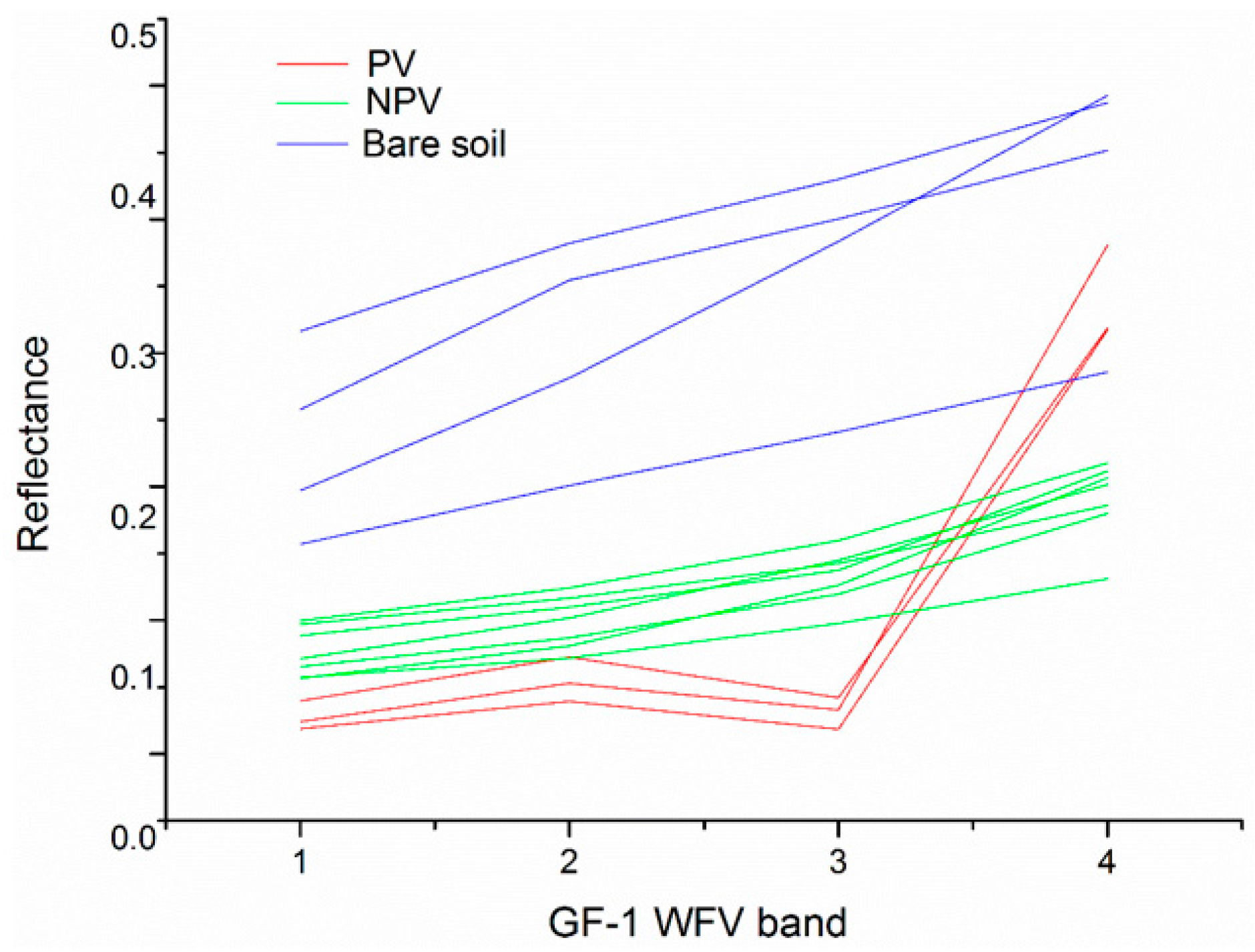
Despite spectral similarity of NPV and bare soil, there are some differences in the GF-1 WFV bands. First and foremost, the bare soil spectra are significantly higher than the NPV spectra, mainly due to extensive bright sandy substrate. In addition, a bow-shaped protuberance exists from blue to red bands in the bare soil spectra, which is not present in the NPV spectra.

(2)

Due to the complex and bright soil background of the Otindag Sandy Land, the bare soil endmember libraries show large intra-variability. Therefore, determining the appropriate endmember combinations, especially the bare soil endmember, is a key process for successfully estimating f_pv and f_npv.

(3)

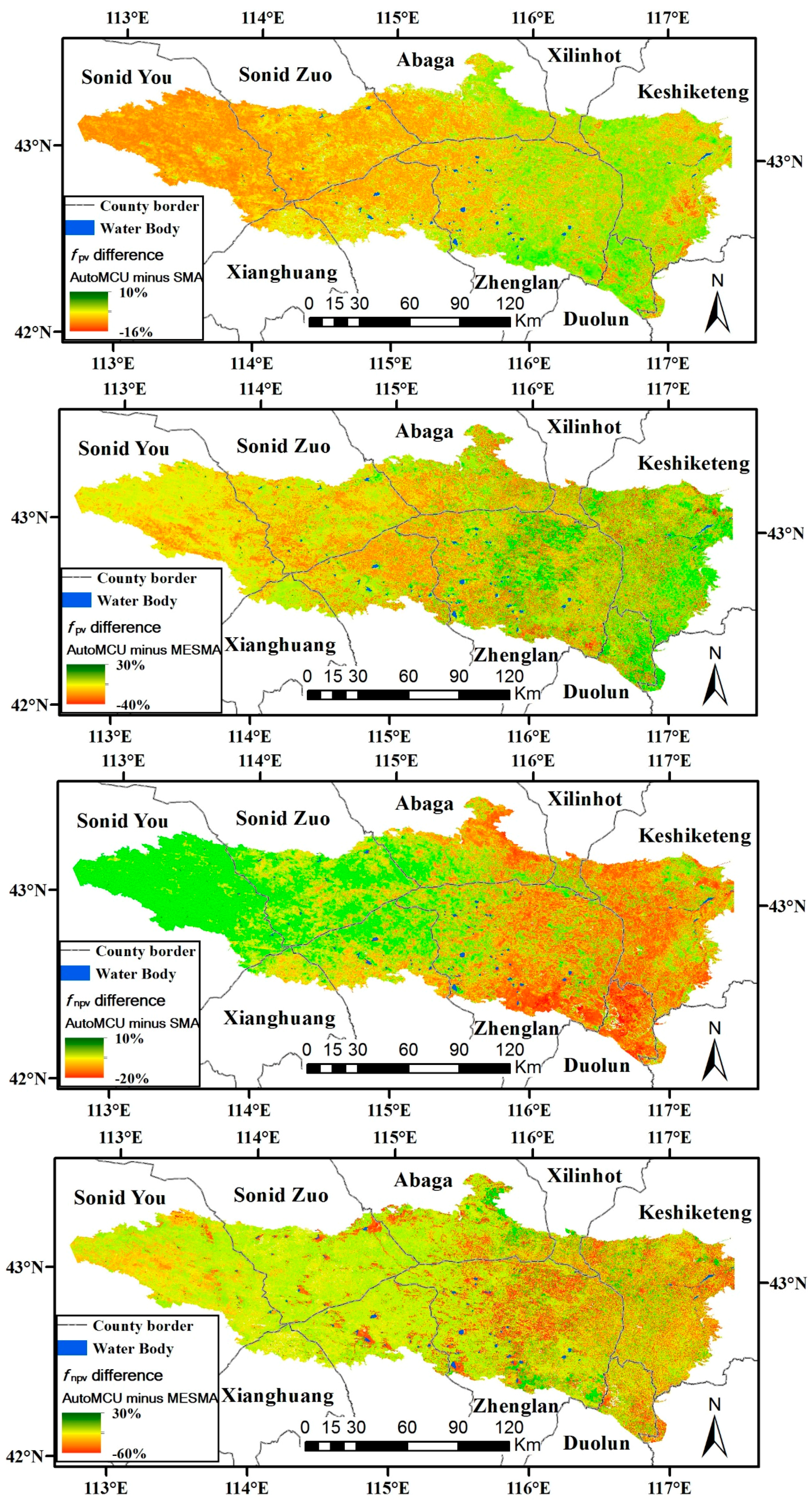
Invariant endmember combinations should be used with caution, because they can lead to serious over- or underestimation problems (SMA). The MESMA cannot be assumed to always perform better than SMA, due to the coupling of the NPV and bare soil endmembers. AutoMCU was shown to be effective for dealing with endmember variability while acquiring accurate f_pv and f_npv estimation. Compared with SMA, both R² and RMSE are improved.

(4)

Compared to other relevant multispectral applications, the GF-1 WFV data were shown to be capable for f_pv and f_npv estimation in the Otindag Sandy Land, despite a lack of the important SWIR bands, which are considered important for separation of NPV from bare soil. With GF-1 WFV’s unique advantage of high spatial resolution (16 m), wide coverage (800 km), and high revisit frequency (2–3 days), there is great potential for future analyses.

References

1. Ruiz-Colmenero, M.; Bienes, R.; Eldridge, D.; Marques, M. Vegetation cover reduces erosion and enhances soil organic carbon in a vineyard in the central Spain. Catena 2013, 104, 153–160. [Google Scholar] [CrossRef]
2. Higginbottom, T.P.; Symeonakis, E. Assessing land degradation and desertification using vegetation index data: Current frameworks and future directions. Remote Sens. 2014, 6, 9552–9575. [Google Scholar] [CrossRef]
3. Asner, G.P.; Heidebrecht, K.B. Imaging spectroscopy for desertification studies: Comparing aviris and eo-1 hyperion in argentina drylands. IEEE Trans. Geosci. Remote Sens. 2003, 41, 1283–1296. [Google Scholar] [CrossRef]
4. Bastin, G.; Scarth, P.; Chewings, V.; Sparrow, A.; Denham, R.; Schmidt, M.; O’Reagain, P.; Shepherd, R.; Abbott, B. Separating grazing and rainfall effects at regional scale using remote sensing imagery: A dynamic reference-cover method. Remote Sens. Environ. 2012, 121, 443–457. [Google Scholar] [CrossRef]
5. Haijiang, L.; Chenghu, Z.; Weiming, C.; En, L.; Rui, L. Monitoring sandy desertification of otindag sandy land based on multi-date remote sensing images. Acta Ecol. Sin. 2008, 28, 627–635. [Google Scholar] [CrossRef]
6. Wu, B.; Li, X.; Liu, W.; Yang, X.; Lu, Q. Desertification control regionalization and rehabilitation counter meatures of source area of sand and dust endangering Beijing–Tianjin. Scientia Silave Sinicae 2006, 42, 65–70. [Google Scholar]
7. Wu, Z.; Wu, J.; Liu, J.; He, B.; Lei, T.; Wang, Q. Increasing terrestrial vegetation activity of ecological restoration program in the Beijing–Tianjin sand source region of China. Ecol. Eng. 2013, 52, 37–50. [Google Scholar] [CrossRef]
8. Li, X.; Zhang, J. Derivation of the green vegetation fraction of the whole China from 2000 to 2010 from MODIS data. Earth Interact. 2016, 20, 1–16. [Google Scholar] [CrossRef]
9. Jiang, Z.; Huete, A.R.; Chen, J.; Chen, Y.; Li, J.; Yan, G.; Zhang, X. Analysis of NDVI and scaled difference vegetation index retrievals of vegetation fraction. Remote Sens. Environ. 2006, 101, 366–378. [Google Scholar] [CrossRef]
10. Gitelson, A.A.; Kaufman, Y.J.; Stark, R.; Rundquist, D. Novel algorithms for remote estimation of vegetation fraction. Remote Sens. Environ. 2002, 80, 76–87. [Google Scholar] [CrossRef]
11. Tucker, C.J. Red and photographic infrared linear combinations for monitoring vegetation. Remote Sens. Environ. 1979, 8, 127–150. [Google Scholar] [CrossRef]
12. Huete, A.; Didan, K.; Miura, T.; Rodriguez, E.P.; Gao, X.; Ferreira, L.G. Overview of the radiometric and biophysical performance of the MODIS vegetation indices. Remote Sens. Environ. 2002, 83, 195–213. [Google Scholar] [CrossRef]
13. Okin, G.S. The contribution of brown vegetation to vegetation dynamics. Ecology 2010, 91, 743–755. [Google Scholar] [CrossRef] [PubMed]
14. Guerschman, J.P.; Hill, M.J.; Renzullo, L.J.; Barrett, D.J.; Marks, A.S.; Botha, E.J. Estimating fractional cover of photosynthetic vegetation, non-photosynthetic vegetation and bare soil in the Australian tropical savanna region upscaling the eo-1 hyperion and MODIS sensors. Remote Sens. Environ. 2009, 113, 928–945. [Google Scholar] [CrossRef]
15. Elmore, A.J.; Asner, G.P.; Hughes, R.F. Satellite monitoring of vegetation phenology and fire fuel conditions in Hawaiian Drylands. Earth Interact. 2005, 9, 1–21. [Google Scholar] [CrossRef]
16. Okin, G.S. Relative spectral mixture analysis—A multitemporal index of total vegetation cover. Remote Sens. Environ. 2007, 106, 467–479. [Google Scholar] [CrossRef]
17. Aguilar, J.; Evans, R.; Daughtry, C. Performance assessment of the cellulose absorption index method for estimating crop residue cover. J. Soil Water Conserv. 2012, 67, 202–210. [Google Scholar] [CrossRef]
18. Daughtry, C.S.; Doraiswamy, P.; Hunt, E., Jr.; Stern, A.; McMurtrey, J., III; Prueger, J. Remote sensing of crop residue cover and soil tillage intensity. Soil Tillage Res. 2006, 91, 101–108. [Google Scholar] [CrossRef]
19. Ren, H.; Zhou, G.; Zhang, F.; Zhang, X. Evaluating cellulose absorption index (CAI) for non-photosynthetic biomass estimation in the desert steppe of Inner Mongolia. Chin. Sci. Bull. 2012, 57, 1716–1722. [Google Scholar] [CrossRef]
20. Jia, G.J.; Burke, I.C.; Goetz, A.F.; Kaufmann, M.R.; Kindel, B.C. Assessing spatial patterns of forest fuel using AVIRIS data. Remote Sens. Environ. 2006, 102, 318–327. [Google Scholar] [CrossRef]
21. Huete, A.R.; Miura, T.; Gao, X. Land cover conversion and degradation analyses through coupled soil-plant biophysical parameters derived from hyperspectral EO-1 hyperion. IEEE Trans. Geosci. Remote Sens. 2003, 41, 1268–1276. [Google Scholar] [CrossRef]
22. Qi, J.; Wallace, O. Biophysical attributes estimation from satellite images in arid regions. In Proceedings of the 2002 IEEE International Geoscience and Remote Sensing Symposium (IGARSS’02), Toronto, ON, Canada, 24–28 June 2002; pp. 2000–2002.
23. Marsett, R.C.; Qi, J.; Heilman, P.; Biedenbender, S.H.; Watson, M.C.; Amer, S.; Weltz, M.; Goodrich, D.; Marsett, R. Remote sensing for grassland management in the arid southwest. Rangel. Ecol. Manag. 2006, 59, 530–540. [Google Scholar] [CrossRef]
24. Cao, X.; Chen, J.; Matsushita, B.; Imura, H. Developing a MODIS-based index to discriminate dead fuel from photosynthetic vegetation and soil background in the asian steppe area. Int. J. Remote Sens. 2010, 31, 1589–1604. [Google Scholar] [CrossRef]
25. Asner, G.P.; Heidebrecht, K.B. Spectral unmixing of vegetation, soil and dry carbon cover in arid regions: Comparing multispectral and hyperspectral observations. Int. J. Remote Sens. 2002, 23, 3939–3958. [Google Scholar] [CrossRef]
26. Okin, G.S.; Clarke, K.D.; Lewis, M.M. Comparison of methods for estimation of absolute vegetation and soil fractional cover using MODIS normalized BRDF-adjusted reflectance data. Remote Sens. Environ. 2013, 130, 266–279. [Google Scholar] [CrossRef]
27. Muir, J. Field Measurement of Fractional Ground Cover: A Technical Handbook Supporting Ground Cover Monitoring for Australia; ABARES: Canberra, Australia, 2011.
28. Roberts, D.A.; Gardner, M.; Church, R.; Ustin, S.; Scheer, G.; Green, R. Mapping chaparral in the Santa Monica Mountains using multiple endmember spectral mixture models. Remote Sens. Environ. 1998, 65, 267–279. [Google Scholar] [CrossRef]
29. Asner, G.P.; Lobell, D.B. A biogeophysical approach for automated SWIR unmixing of soils and vegetation. Remote Sens. Environ. 2000, 74, 99–112. [Google Scholar] [CrossRef]
30. Heinz, D.C.; Chang, C.-I. Fully constrained least squares linear spectral mixture analysis method for material quantification in hyperspectral imagery. IEEE Trans. Geosci. Remote Sens. 2001, 39, 529–545. [Google Scholar] [CrossRef]
31. Chang, C.-I.; Heinz, D.C. Constrained subpixel target detection for remotely sensed imagery. IEEE Trans. Geosci. Remote Sens. 2000, 38, 1144–1159. [Google Scholar] [CrossRef]
32. Gao, Z.; Bai, L.; Wang, B.; Li, Z.; Li, X.; Wang, Y. Estimation of soil organic matter content in desertified lands using measured soil spectral data. Scientia Silvae Sinicae 2011, 47, 9–16. [Google Scholar]
33. Numata, I.; Roberts, D.A.; Chadwick, O.A.; Schimel, J.; Sampaio, F.R.; Leonidas, F.C.; Soares, J.V. Characterization of pasture biophysical properties and the impact of grazing intensity using remotely sensed data. Remote Sens. Environ. 2007, 109, 314–327. [Google Scholar] [CrossRef]
34. Ballantine, J.-A.C.; Okin, G.S.; Prentiss, D.E.; Roberts, D.A. Mapping north african landforms using continental scale unmixing of MODIS imagery. Remote Sens. Environ. 2005, 97, 470–483. [Google Scholar] [CrossRef]
35. Mishra, N.B.; Crews, K.A. Estimating fractional land cover in semi-arid central kalahari: The impact of mapping method (spectral unmixing vs. Object-based image analysis) and vegetation morphology. Geocarto Int. 2014, 29, 860–877. [Google Scholar] [CrossRef]
36. Okin, G.S.; Roberts, D.A.; Murray, B.; Okin, W.J. Practical limits on hyperspectral vegetation discrimination in arid and semiarid environments. Remote Sens. Environ. 2001, 77, 212–225. [Google Scholar] [CrossRef]
37. Davidson, E.A.; Asner, G.P.; Stone, T.A.; Neill, C.; Figueiredo, R.O. Objective indicators of pasture degradation from spectral mixture analysis of Landsat imagery. J. Geophys. Res. Biogeosci. 2008, 113. [Google Scholar] [CrossRef]
38. Asner, G.P.; Levick, S.R.; Smit, I.P. Remote sensing of fractional cover and biochemistry in savannas. In Ecosystem Function in Savannas: Measurement and Modelling at Landscape to Global Scales; CRC Press: Boca Raton, FL, USA, 2011; pp. 195–218. [Google Scholar]
39. Harris, A.T.; Asner, G.P. Grazing gradient detection with airborne imaging spectroscopy on a semi-arid rangeland. J. Arid Environ. 2003, 55, 391–404. [Google Scholar] [CrossRef]
40. Zare, A.; Ho, K. Endmember variability in hyperspectral analysis: Addressing spectral variability during spectral unmixing. IEEE Signal Proc. Mag. 2014, 31, 95–104. [Google Scholar] [CrossRef]
41. Asner, G.P.; Knapp, D.E.; Cooper, A.N.; Bustamante, M.M.; Olander, L.P. Ecosystem structure throughout the Brazilian Amazon from Landsat observations and automated spectral unmixing. Earth Interact. 2005, 9, 1–31. [Google Scholar] [CrossRef]
42. Guerschman, J.P.; Oyarzabal, M.; Malthus, T.; McVicar, T.; Byrne, G.; Randall, L.; Stewart, J. Evaluation of the MODIS-Based Vegetation Fractional Cover Product; Commonwealth Scientific and Industrial Research Organization (CSIRO): Canberra, Australia, 2012.
43. Guerschman, J.P.; Scarth, P.F.; McVicar, T.R.; Renzullo, L.J.; Malthus, T.J.; Stewart, J.B.; Rickards, J.E.; Trevithick, R. Assessing the effects of site heterogeneity and soil properties when unmixing photosynthetic vegetation, non-photosynthetic vegetation and bare soil fractions from Landsat and MODIS data. Remote Sens. Environ. 2015, 161, 12–26. [Google Scholar] [CrossRef]
44. Qu, L.; Han, W.; Lin, H.; Zhu, Y.; Zhang, L. Estimating vegetation fraction using hyperspectral pixel unmixing method: A case study of a karst area in China. IEEE J. Sel. Top. Appl. Earth Obs. Remote Sens. 2014, 7, 4559–4565. [Google Scholar] [CrossRef]
45. Mu, X.; Hu, M.; Song, W.; Ruan, G.; Ge, Y.; Wang, J.; Huang, S.; Yan, G. Evaluation of sampling methods for validation of remotely sensed fractional vegetation cover. Remote Sens. 2015, 7, 16164–16182. [Google Scholar] [CrossRef]
Figure 1. Location of the study area in North China.
Remotesensing 08 00800 g001
Figure 2. Photos of major vegetation structure and characteristics in the Otindag Sandy Land: (a) open woodland; (b) grassland encroached by shrub; (c) degraded grassland; and (d) high percentage of non-photosynthetic vegetation (NPV).
Remotesensing 08 00800 g002
Figure 3. Endmember spectra of (a) Photosynthetic vegetation (PV); (b) Non-photosynthetic vegetation (NPV) and (c) Bare soil used in Spectral Mixture Analysis (SMA), the filled squares are the average values of different types.
Remotesensing 08 00800 g003
Figure 4. fpv, fnpv and fsoil estimation based on: (a) Spectral Mixture Analysis (SMA); (b) Multi-Endmember Spectral Mixture Analysis (MESMA) and (c) Automated Monte Carlo Unmixing Analysis (AutoMCU).
Remotesensing 08 00800 g004
Figure 5. fpv, fnpv and fsoil estimation accuracy validation against field samples.
Remotesensing 08 00800 g005
Figure 6. fpv (a); and fnpv (b) distribution and their average values relative to unmixing iterations using Automated Monte Carlo Unmixing Analysis (AutoMCU).
Remotesensing 08 00800 g006
Figure 7. Photosynthetic vegetation (PV), Non-photosynthetic vegetation (NPV) and bare soil endmember variability in Multi-Endmember Spectral Mixture Analysis (MESMA).
Remotesensing 08 00800 g007
Figure 8. fpv and fnpv differences based on Spectral Mixture Analysis (SMA), Multi-Endmember Spectral Mixture Analysis (MESMA) and Automated Monte Carlo Unmixing Analysis (AutoMCU).
Remotesensing 08 00800 g008