Article

Landsat and Local Land Surface Temperatures in a Heterogeneous Terrain Compared to MODIS Values

by
Gemma Simó
1,
Vicente García-Santos
1,2,
Maria A. Jiménez
1,*,
Daniel Martínez-Villagrasa
1,
Rodrigo Picos
1,
Vicente Caselles
2 and
Joan Cuxart
1
1
Departament de Física, Universitat de les Illes Balears, Cra. Valldemossa km. 7.5, Palma 07122, Spain
2
Departament de Física de la Terra i Termodinàmica, Universitat de València, València 46010, Spain
*
Author to whom correspondence should be addressed.
Submission received: 9 August 2016 / Revised: 29 September 2016 / Accepted: 11 October 2016 / Published: 15 October 2016

Abstract

:
Land Surface Temperature (LST) as provided by remote sensing onboard satellites is a key parameter for a number of applications in Earth System studies, such as numerical modelling or regional estimation of surface energy and water fluxes. In the case of Moderate Resolution Imaging Spectroradiometer (MODIS) onboard Terra or Aqua, pixels have resolutions near 1 km 2 , LST values being an average of the real subpixel variability of LST, which can be significant for heterogeneous terrain. Here, we use Landsat 7 LST decametre-scale fields to evaluate the temporal and spatial variability at the kilometre scale and compare the resulting average values to those provided by MODIS for the same observation time, for the very heterogeneous Campus of the University of the Balearic Islands (Mallorca, Western Mediterranean), with an area of about 1 km 2 , for a period between 2014 and 2016. Variations of LST between 10 and 20 K are often found at the sub-kilometre scale. In addition, MODIS values are compared to the ground truth for one point in the Campus, as obtained from a four-component net radiometer, and a bias of 3.2 K was found in addition to a Root Mean Square Error (RMSE) of 4.2 K. An indication of a more elaborated local measurement strategy in the Campus is given, using an array of radiometers distributed in the area.

Graphical Abstract

1. Introduction

Land Surface Temperature (LST) is the radiative temperature of the most superficial part of the soil and vegetation of an element of the surface, sometimes also referred to as the skin temperature of the surface [1]. Temperature usually varies very significantly with a height from this interface upwards in the lowest meters of the atmosphere [2], and the same happens as the progressively deeper layers in the soil are explored [3], with variations of contrary signs, with usually LST being the highest (lowest) value of the temperature profile in the daytime (nighttime). In applications, LST is usually taken as a boundary condition for atmosphere or for the soil and the surface fluxes estimated using its values are the main drivers of the physical processes involved in the surface energy and water balances ([4,5,6,7,8]). An adequate spatial and temporal characterization of LST is needed to properly understand the contributions of the different terms in these surface budgets [9].
Since this layer is in contact with two media at the same time (atmosphere and soil/vegetation), it is very difficult to make a meaningful measurement of the temperature using a thermometer [10]. Instead, LST is determined by measuring the amount of energy radiated by the surface, determined by a radiometer. Land and vegetation emit longwave radiation and, therefore, LST is estimated by means of Thermal infrared (TIR) sensors, using the Stefan–Boltzmann relation for a black body—modified with the emissivity of the surface—and subtracting the downward longwave radiation reflected upward. LST is currently determined from satellite or direct in situ radiometric measurements.
If LST is obtained from the Atmospheric Surface Layer (ASL), which is a layer of air with a thickness of a few meters above the surface, there are a number of well identified issues that influence LST measurements: (i) the very small scale heterogeneities [11], implying that the radiometer receives radiation from elements of the surface radiating differently; (ii) the determination of the emissivity of the emitting surface, which strongly depends on the amount of water in the upper centimetres of the soil and the state of the vegetation, and, nonetheless; (iii) the possible high-concentration of atmospheric emitters between the radiometer and the surface, such as CO 2 and water vapour, especially on stable nights. The usual strategies are to sample homogeneous surfaces, to determine the emissivity of the sampled area and to measure the radiation emitted through a window partially transparent to CO 2 and to water vapour.
When a radiometer is onboard a satellite, the same limitations as if the sensor was in the ASL exist, but their effect is severely amplified. Depending on the sensor and the height of the orbit, the resolution may vary between some decametres (as for Landsat 7 Enhanced Tematic Mapper plus, ETM+) and one to few kilometres (the case of Moderate Resolution Imaging Spectroradiometer (MODIS) onboard Aqua and Terra or Spinning Enhanced Visible and InfraRed Imager (SEVIRI) onboard Meteosat Second Generation). It is clear that the surface heterogeneities at these scales will be very important depending on the type of surface, and the average value of the pixel may be significantly different from a point measurement on the ground.
A disadvantage for satellite-derived LST is that normally high spatial resolution (60 m for Landsat 7 ETM+ against 1000 m for Terra MODIS) supposes low temporal frequency (several days for ETM+ against two per day for MODIS), so in situ measurements are needed to fulfill the spatial and temporal gaps of current orbiting TIR sensors. Most studies comparing satellite measurements and direct measurements of LST occur in homogeneous areas ([12,13,14,15,16,17,18]; etc.). There are a few studies for heterogeneous areas, like the downscaling ones of [19,20] between MODIS and ETM+ sensors, or LST validation campaign of [16,21,22] where LST satellite data was compared with in situ measurements. It is usually concluded that errors are higher in heterogeneous areas than in homogeneous ones (a summary is shown in Table 1). All these validation works have demonstrated good operational performance of the three MODIS LST algorithms at different surface types with discrepancies respect to reference data of around 1 K. However, the coarser spatial resolution of the MODIS TIR bands is not probably the most suitable for other research goals, which demand LST data at sub-kilometer resolution.
Emissivity may also vary largely along the pixel, especially depending on the distribution of water in the ground, the soil materials and the vegetation cover. Finally, since practically the whole atmosphere is between the emitting surface and the receiver, the correction of the longwave emission by the atmospheric compounds is compulsory.
To use LST values given by a sensor onboard a satellite, these must have gone through processes of validation and calibration that provide an estimation of the uncertainty of the value. This information is obtained primarily with ground-based data used for comparison, usually for ground homogeneous conditions. However, validation studies for heterogeneous terrains are more difficult [23] and they are more rarely found in the literature. Furthermore, the suitability of a point measurement for verification is in question in these conditions. It may well happen that the pixel-averaged value or the local measurement point are in fact not representative of the actual conditions governing the surface atmosphere exchanges over each of the subpixel tiles. This would be important since it could provide inadequate values of surface temperature or sensible and latent energy fluxes for numerical models or agricultural applications [24].
In this work, the average values for the MODIS pixel centered on the Campus of the University of the Balearic Islands, very heterogeneous, will be compared to the averaged values computed from available Landsat 7 images (one every seven to nine days), at 30 m resolution (disaggregated from 60 m by the Landsat Team) for a period of 2.5 years. The representativity of the MODIS average value will be assessed, and an estimation of the subpixel variability provided. Furthermore, the radiometric data obtained at one spot of the Campus will be compared to the MODIS value and to the corresponding Landsat 7 pixel, allowing assess to the possible discrepancies made in the validation results when taking these three quantities as equivalent.

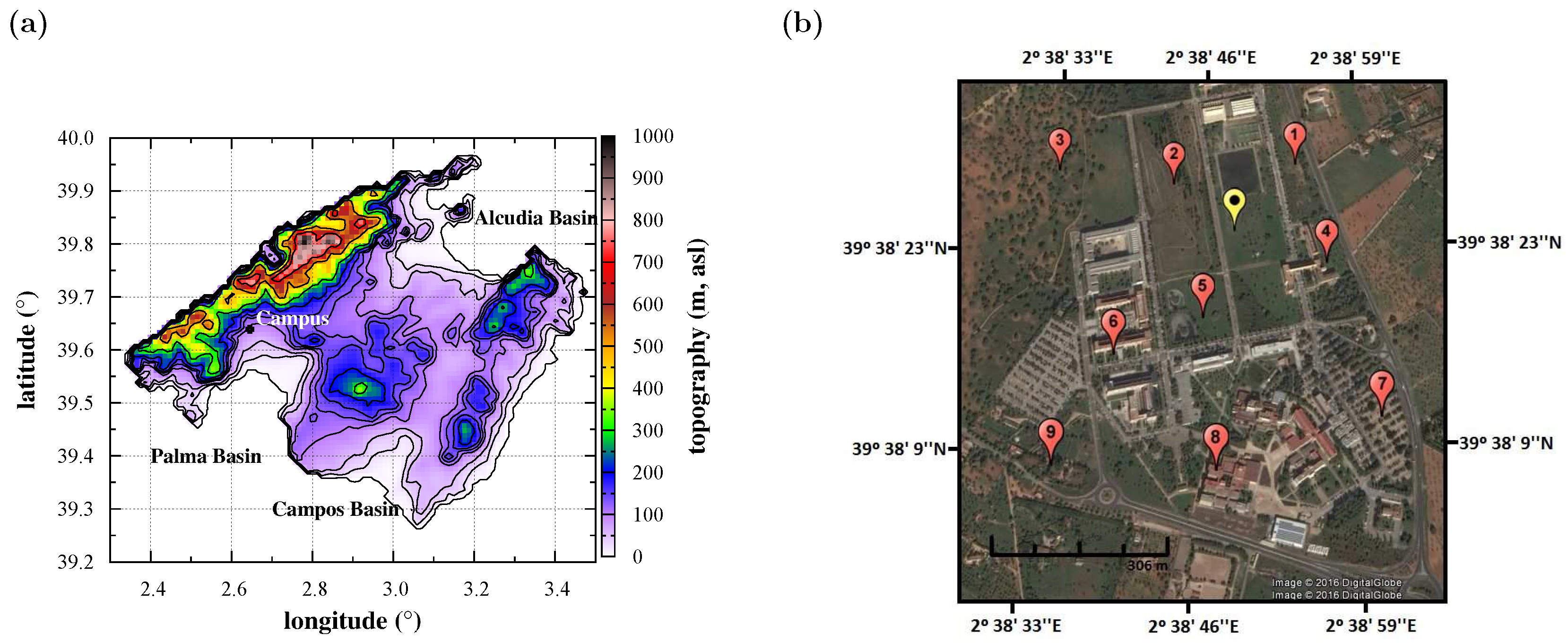
2. Description of the Site and Tools

The study site is placed in Mallorca (Figure 1a), the largest of the Balearic Islands, located in the Western Mediterranean Sea, 200 km east of the Iberian Peninsula. The Campus of the University of the Balearic Islands (UIB, indicated in Figure 1a) has been taken in this study as an example of heterogeneous area. It is located in the west of the island, in the Palma basin, at the foothills of the northern mountain range (Serra de Tramuntana). The UIB Campus has an approximate area of 1 km 2 with heterogeneous terrain composed of many different types of surfaces such as buildings, asphalted roads, terrain slopes, farmed areas with green vegetables or orange and almond trees, wet grass, drier extensions, etc. (Figure 1b). Previous studies ([25,26]) showed that during high-pressure gradient and clear sky conditions, locally generated winds are present in Mallorca and especially in the three main basins. This is the case for the diurnal sea-breeze (especially from April to October) or the nocturnal land-breeze which is often coupled with downslope winds.
A complete surface energy budget station (yellow dot in Figure 1b), operating at the UIB Campus since January 2015, is used in this study as a ground reference value of LST measurement for satellite validation purposes. In addition, a total of nine different points were selected inside the UIB Campus as representative of the different type of surfaces mentioned above (see red dots in Figure 1b). Designated points 1, 3, 4, and 9 are in the midst of almond trees, orange trees, carob trees and fields of different crops, respectively. These reference points are representative of the fields that are also surrounding the Campus. Points 2 and 5 are over a gully usually with wet soil, the latter next to a pond. Points 6 and 8 are surrounded by buildings and point 7 is in a parking lot.
LST fields used in this work are taken from two types of sensors: (i) MODIS onboard the Terra and Aqua platforms and (ii) ETM+ onboard the Landsat 7 platform. These satellites have been chosen because of the availability of the images (free and easy to access) and especially because both cover our study site at two different spatial and temporal resolutions. Images for clear sky days from 1 January 2014 to 1 June 2016 over the Campus area are taken in the analysis.

2.1. Landsat 7 ETM+ Land-Surface Temperatures

Landsat 7 has a heliosynchronous polar orbit, which is completed in about 99 min, allowing the satellite to make fourteen rounds on Earth per day and cover the entire planet in 16 days. Due to the location of the island of Mallorca, Landsat 7 passes over it every 7–9 days at approximately at 10:30 UTC because the island is placed between the passage of two different orbits of Landsat 7. Therefore, we get a higher temporal resolution in the study area than in other regions. ETM+ measures the radiance in eight spectral bands ranging from the visible spectrum to TIR range with a spatial resolution of 30 m (disaggregated from 60 m by the Landsat Team in the case of the TIR band). It also has a panchromatic band at 15 m spatial resolution. A failure in the Scan Line Corrector (SLC-off mode) occurred in 2003 and has affected, since that year, the scenes of the Landsat 7, generating void-data bands of a width near 100 m every kilometre.
Retrieval of LST from Landsat 7 ETM+ is based on the single-channel method ([27]), which corrects the Top of Atmosphere (TOA) spectral radiance measurements performed by the ETM+ at band 6 (10–12 μ m), from atmospheric attenuation and surface emission. LST variable is cleared from the Radiative Transfer Equation (RTE) in (1)
L T O A , i = [ ϵ i B i ( L S T ) ( 1 ϵ i ) L h e m , i ] τ i + L a t m , i ,
where L T O A , i (in W·sr 1 ·m 2 · μ m 1 ) is the TOA radiance measured by the ETM+ sensor, ϵ i is the surface emissivity, B i ( L S T ) is the Planck function of a blackbody emitting at the surface temperature (LST) and L h e m , i , τ i and L a t m , i are the atmospheric parameters corresponding to hemispherical downwelling radiance, atmosphere transmissivity and upwelling radiance, respectively. Subscript i refers to the channel-effective quantity of each parameter in the RTE (e.g., band 6 (10–12 μ m) of the ETM+ in this case).
L T O A , i in Equation (1) is calculated with the conversion of the Digital Number ( D N ) measured from band 6 of the ETM+ to radiance, following (Landsat 7 Science Data Users Handbook, [28])
L T O A , i = 0.037 D N + 3.1628 .
The surface emissivity used in Equation (1) was extracted from the Advanced Spaceborne Thermal Emission and Reflection Radiometer (ASTER) Global Emissivity Database (GED) ([29]). This database offers surface emissivity values at 100 m 2 spatial resolution for the five TIR channels of the ASTER sensor ([30]) after applying the Temperature and Emissivity Separation method ([31]) to the ASTER data from 2000 to 2008. In this study, the emissivity used to correct the surface emission at the disaggregated TIR image of the ETM+ sensor at 30 m× 30 m pixel, was calculated from the mean value of the ASTER GED emissivities in channels 13 (10.25–10.95 μ m) and 14 (10.95–11.65 μ m), since both channels cover the spectral resolution of the band 6 in ETM+ Landsat 7 sensor. We obtained a range of emissivities of 0.960–0.982 for the area of study, with an average of 0.972 and 0.004 deviation (this is shown in Figure 2b as an example for 8 November 2015). With this procedure, the associated uncertainty is about 0.015 and therefore LST values might also have an uncertainty of about 1.5 K [31]. In situ observations of the surface emissivity at the UIB Campus are needed to have more realistic emissivity values to reduce the uncertainty in the derivation of LST products.
Atmospheric variables in RTE were calculated with the MODerate resolution atmospheric TRANsmission (MODTRAN) radiative transfer code (v. 5.2.1, [32]) using as input the atmospheric profile modeled with the web-tool calculator implemented by [33]. This simulated profile is interpolated spatially and temporally to the selected site and it is representative of the atmosphere in a 1 spatial resolution. This atmospheric profile was demonstrated to be the best option to correct the atmospheric effect compared with other profiles like that offered by the MOD07 product [34].
Once the variable B i ( L S T ) in the RTE is cleared, LST is obtained with the expression proposed in the Landsat 7 Science Data Users Handbook [28] to convert radiance to temperature (in K) at band 6 as:
L S T = 1282.71 l n ( 666.09 B i ( L S T ) + 1 ) .
For the studied area (1 km 2 centered in the UIB Campus, Figure 1b) and period (January 2014–May 2016), a total of 63 ETM+ scenes are used corresponding to clear-sky conditions, providing LST fields at around 10:30 UTC.

2.2. The Terra MODIS Land-Surface Temperatures

The Terra MODIS satellite was launched in 1999, and, since then, it has provided global coverage, offering twice-daily LST and emissivity products generated from three different algorithms: the MOD11 L2 (and Level 3 MOD11A1) using the generalized split-window (GSW) algorithm [35], the MOD11B1 with the physically based day/night (D/N) algorithm [36] and the new MOD21 LST and emissivity (MODTES) product [37] adapted from the temperature-emissivity separation (TES) method [31] and the water vapor scaling (WVS) method [38] for refined atmospheric correction. First validation works of the MODIS LST product have been published since very soon after its launch for the first proposed GSW method ([39,40,41]). The D/N method has also been validated [42], and, more recently, the MODTES LST product has been validated in several studies ([14,15]).
MODIS has a polar orbit covering all of the Earth every one or two days. Terra MODIS passes over, in its ascending orbit, the Balearic Islands (39 N, 3 E) every day between 10:00 and 11:00 UTC acquiring data in its 36 spectral bands, at approximately the same instant as ETM+, with LST fields at a spatial resolution of 1 km × 1 km. The collection 5 and Level 3 of MOD11A1 daily LST product ([43]) is selected, which provides LST values at 1 km spatial resolution gridded in the Sinusoidal projection. The LST product is generated by the generalized split-window LST algorithm ([35]).
A total of 469 Terra MODIS scenes are used in this work covering the period of (January 2014–May 2016) with clear-skies in the UIB Campus (Figure 1b) at approximately the same instant as those obtained from ETM+. Therefore, a direct comparison of the corresponding LST fields is possible.

2.3. In Situ LST Field Data

The ground-measured LST is calculated with a Hukseflux RN01 net radiometer (Delft, The Netherlands) installed at the reference measuring point. This sensor provides the four terms of the radiation budget at the Earth’s surface. It consists of a pair of pyranometers facing upward and downward to measure the surface down and upwelling shortwave radiation terms, respectively, while two pyrgeometers are similarly located to measure the far-infrared longwave radiation contribution, within a spectral range of 4.5–50.0 μ m. The field of view (FOV) for both pyrgeometers is 150 (180 for the pyranometers). Therefore, considering that the RN01 radiometer is located at 1 m height, the measured upwelling longwave radiation corresponds to a surface area with a diameter of 7.5 m. The terrain in this part of the area of study is homogeneous for an extension of several tens of meters.
In order to obtain the in situ LST, the measured upwelling longwave radiation L must be corrected from the reflected downwelling contribution L , following the expression:
L S T = L ( 1 ε ) L ) ε · σ 1 / 4 ,
where ε = 0.97 is the surface broadband emissivity, a value taken from [44] corresponding to senescent sparse shrubs, a common soil type of the UIB Campus. σ = 5.67 × 10 8 W · m 2 · K 4 represents the Stefan–Boltzmann constant, L↑ and L↓ are in W·m 2 and LST in K.
The data used for the ground-based observations correspond to the 1 min average measured every day at 10:30 UTC from 1 January 2015 to 1 June 2016. The time of the day is selected according to the pass time of the satellites involved in this study to minimize the temporal mismatch between the three observational sources. The radiation instrument was calibrated by the manufacturer in June 2013, and it was mounted for the first time in January 2015. Data quality control has been performed since then by cleaning the sensor domes periodically and critically reviewing the measured data.

2.4. Previous Validations of Satellite-Derived LST

Table 1 shows the results from recent studies where the satellite LST is validated using ground-based measurements over different surface types. The selected works report products from MODIS and Landsat 7 ETM+ and retrieve LST using a variety of algorithms and methods to deal with atmospheric and emissivity effects. When possible, the biases and RMSEs included in Table 1 correspond specifically to the same satellite products used in the current study. For MODIS, most of the results included correspond to cases where the gridded (Level 3) product MOD11A1 in its collection 5 was used ([12,13,14,22]), although ([15,16], and [13] for the rice crop area) the swath product MOD11_L2 was used, which is prior to the gridded one. For the ETM+ studies [18], local-radiosonde profiles were used to retrieve the atmospheric parameters in RTE instead of the synthetic ones generated by the web-tool calculator described in Section 2.1, while [17] compared both methodologies over a homogeneous surface, obtaining better results for the interpolated profiles.
Regarding the ground truth calculation, different instruments and methods were applied depending on the study. Generally, averages from several ground measurements taken over different parts of the area of interest were preferred ([12,15,16,17,18,22]), although [22] obtained better results with a single measurement from a four-component net radiometer located at 6 m height over a strong heterogeneous site. Ref. [13] uses a single thermal-infrared radiometer that measured at different observation angles, while [14] built the ground truth LST after identifying the fractions of the main surface elements seen by the on-board sensor.
All the studies in Table 1 show that MODIS products underestimate LST compared to ground-based measurements (despite of the method used to calculate the in situ LST) and the bias is larger over more heterogeneous surfaces. Similarly, bias and associated RMSE increase during the day, when spatial thermal differences are larger. ETM+ products do not seem to improve the MODIS results over homogeneous surfaces (see, for instance, bias and errors from [15,17] in Table 1, both studies performed at the same site in summer time). In the following section, we will evaluate what the results are over a heterogeneous surface.

3. Results

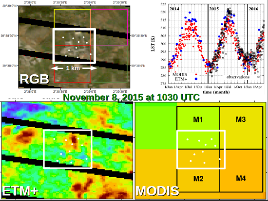
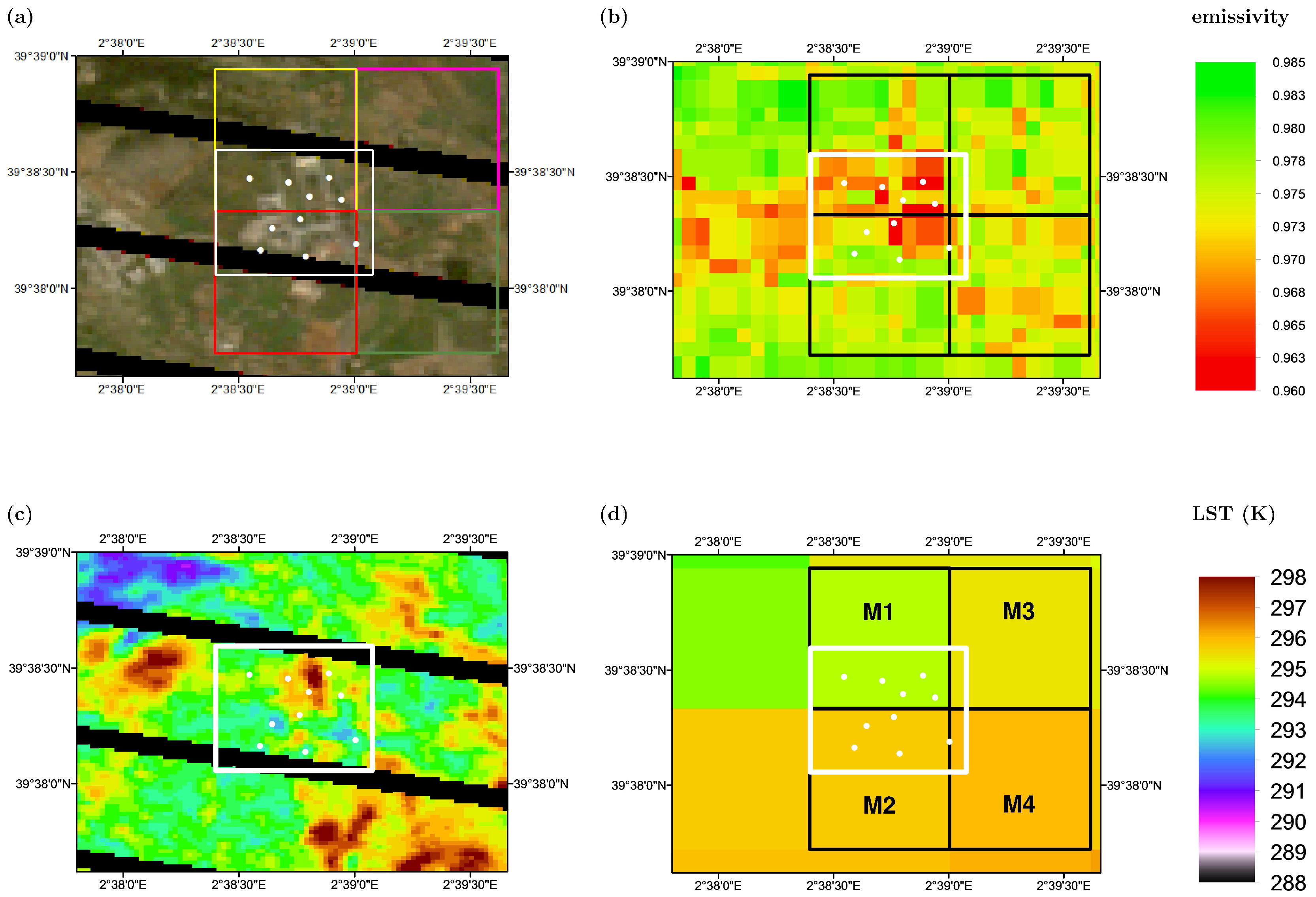
3.1. Spatial Variability of LST Fields

An example of LST difference between ETM+ and MODIS products is shown in Figure 2, for a scene from 8 November 2015 at 10:30 UTC. Let us remind readers here about the no-data bands as introduced above. Figure 2a is a true color composite of a Landsat 7 scene centered on the UIB Campus and surroundings: R (Band 3, 0.63–0.69 μ m), G (Band 2, 0.52–0.60 μ m) and B (Band 1, 0.45–0.52 μ m). Figure 2b shows the average emissivity of ASTER TIR bands 13 and 14. The UIB Campus is defined with a white square that consists of 33 × 33 Landsat 7 ETM+ pixels (a total of 1089 pixels) at 30 m spatial resolution (Figure 2c, corresponding to the disaggregated TIR scene from the original 60 m spatial resolution). Therefore, the averaged Landsat 7 ETM+ LST at the UIB Campus is computed from the values of Landsat 7 included in the 1 km 2 of the Campus without considering the data inside the black bands. On the other hand, four pixels of MOD11A1 are partially included in the UIB square (M1, M2, M3 and M4 in Figure 2d), and the averaged MOD11A1 LST is the weighted average of these four pixels (44% for M1 and M2 and 6% for M3 and M4).
Figure 2c shows, for the same Landsat 7 scene of Figure 2a, the LST map calculated with the single-channel method explained in Section 2.1. Differences as large as 15 K can be seen in the full image and up to 12 K just in the area corresponding to the UIB Campus, marked with a white square. The warmer area corresponds to a soccer field covered by artificial grass, while the coldest areas are located close to buildings in the Campus.
The corresponding MOD11A1 LST (6 pixels at 1 km 2 ) is seen in Figure 2d for the same day and time of the Landsat 7 scene in Figure 2c, and painted with the same color palette. In this case, there is a difference of 1.4 K in the whole picture and 1.2 K in the UIB pixel. Therefore, in this single scene, it is checked that with lower spatial resolution (1 km 2 ), significant temperature gradients at the hectometre scale are not detectable, pointing to the need of higher horizontal resolution fields to monitor their evolution, something currently out of reach with the satellites at disposal for the scientific community that have these images just once every several days and for a single instant. However, heterogeneities of this size may contribute significantly to measured surface energy and water budgets over land, according to other previous studies ([11]).

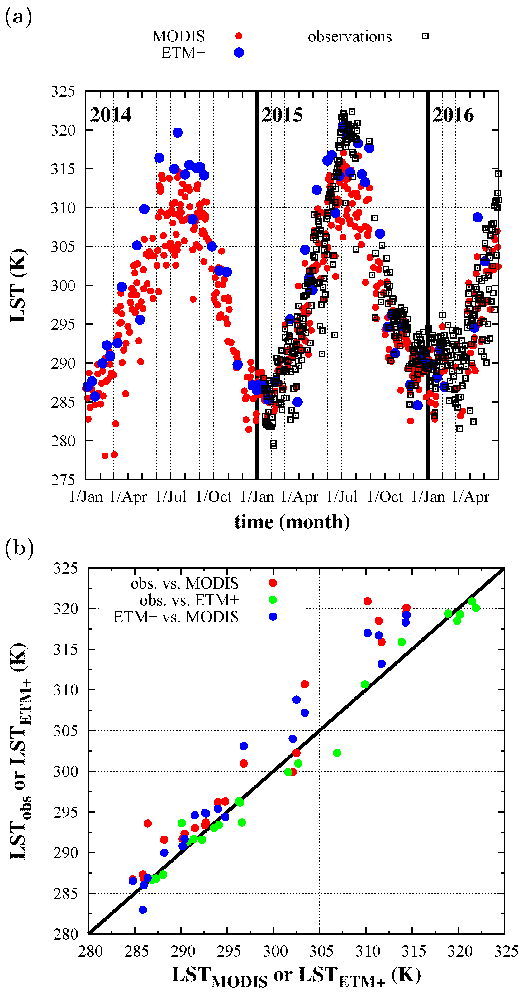
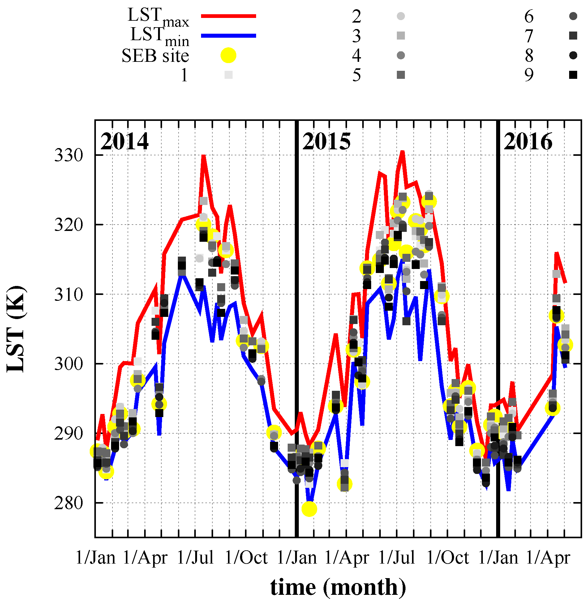
3.2. Annual Evolution of LST

After exploring the heterogeneities for one single scene, the evolution of LST is shown in Figure 3a for the period January 2014–May 2016. Figure 3a represents the annual evolution of LST for Landsat 7 ETM+ (averaged value of the 1089 pixels included in the 1 km 2 in Figure 2c, see Section 2.1), Terra MODIS (four pixels’ weighted average as indicated in Section 3.1) and the ground-based measurements (derived from the longwave radiation components as seen in Section 2.3) taken at the reference station (starting on 1 January 2015). At the scale displayed in the graph, there is good agreement between the three data sources; however, discrepancies on the order of 5 K are common, and they can rise up to 10 K in summer.
To have a first quantification of the discrepancies, Figure 3b shows the comparison between pairs of LST temperatures. A total of 24 days are used in Figure 3b when MODIS, ETM+ and in situ measurements are available at about 10:30 UTC (only covering the period January 2015–May 2016, limited by the temporal interval when in situ measurements were taken).
The first noteworthy issue is that the Landsat 7 30 m size pixel LST value closest to the measurement site compares very well to the observed LST in situ value for the whole range of observed temperatures (r 2 = 0.98, bias = −0.5 K and RMSE = 1.7 K). This indicates that LST variability at scales under 30 m is not very large in this region of the UIB Campus. Discrepancy between the observed in situ value and the closest MODIS pixel is relatively small below 305 K (on the order of 1–3 K) and increases to 5 K or more for higher temperatures (r 2 = 0.95, bias = 3.2 K and RMSE = 4.2 K for the whole temperature range). In hot weather, LST variability seems to be very large and the point measurement may be a poor surrogate of the pixel-average value. Similar results are found when Landsat 7 and MODIS LST values averaged over the UIB Campus are compared (r 2 = 0.98, bias = 2.5 K and RMSE = 3.1 K). It is worth noting that the effect of surface emissivity accounts for a significant part of the discrepancies on LST found between MODIS and an appropriate average of Landsat LST over the site. It is known that the MOD11A1 LST product in its collection 5 presents too emissivity values that are too high [39]. Thus, this could be an important cause of such discrepancies between the two sensors, particularly in summer, when LST values are higher and emissivity is lower due to surface drying.
The preliminary conclusions are that (i) Landsat 7 is an adequate tool to compute the variability of LST at the sub-kilometre scale, since it compares very well with local data; (ii) the uncertainty in the computation of LST product is smaller than the variability of these fields over the UIB Campus and (iii) for LST below 300 K the three estimations seem to be of similar quality, with MODIS diverging significantly for higher temperatures.
Uncertainties and biases obtained in the present study are consistent with those obtained in previous studies (see Table 1) for both satellite products analyzed here. In our case, these discrepancies are slightly larger, most likely because of the heterogeneities of the terrain ([22]) and also because the ground truth is built with a single-point measurement with a reduced FOV of 7.5 m. Land surface heterogeneities lead to strong LST differences during daytime, as seen in [14,16,22]. This effect is also evident during the year, where discrepancies between satellite and single-point ground measurements increase in summer. It is important to take into account the source of the differences shown in Figure 3b such as: (i) the different algorithms (and assumptions considered) to derive LST for MODIS, ETM+ and the radiometer; (ii) the area representative of the pixel (for MODIS and ETM+) and the representativeness of the single-point measurement, especially in such an heterogeneous place; (iii) differences in emissivity may induce temperature differences of about 1.5 K [31] (or higher due to emissivity overestimation in the algorithm of the MOD11A1 LST product commented on previously), but, in any case, this difference is lower than the temperature variability typically reported in the Campus area (see, for instance, Figure 2c) during the studied period; and (iv) the 30 min temporal mismatch between MODIS and Landsat 7 overpass could be a significant factor in the LST difference between both sensors that could reach a value up to 1.5 K in hot weather conditions [45].
To inspect the spatial variability within the UIB Campus and assess how representative a single station would be, the values of the 10 points with different surface characteristics and representative of the UIB Campus variability are taken (Figure 1b, one of them is placed in the measurement site). Figure 2c shows that they are located in points with very different LSTs. Figure 4 shows the temporal evolution of the maximum Landsat 7 ETM+ LST (red line) and minimum (blue line) values for the entire study area (Campus UIB, Figure 1b). Individual LSTs for each of these ten points are also included. Along the 2.5 years represented, the maximal LST range for the UIB pixel is found in the summer, when it is between 15 and 20 K, while it is reduced to 5–10 K in the cold seasons. The spread of points between the lines indicates that the selected locations cover well the thermal variability within the 1 km 2 studied area of the Campus. These selected points may be considered for taking in situ measurements and building a more accurate ground truth LST to compare against satellite products in a future research action.

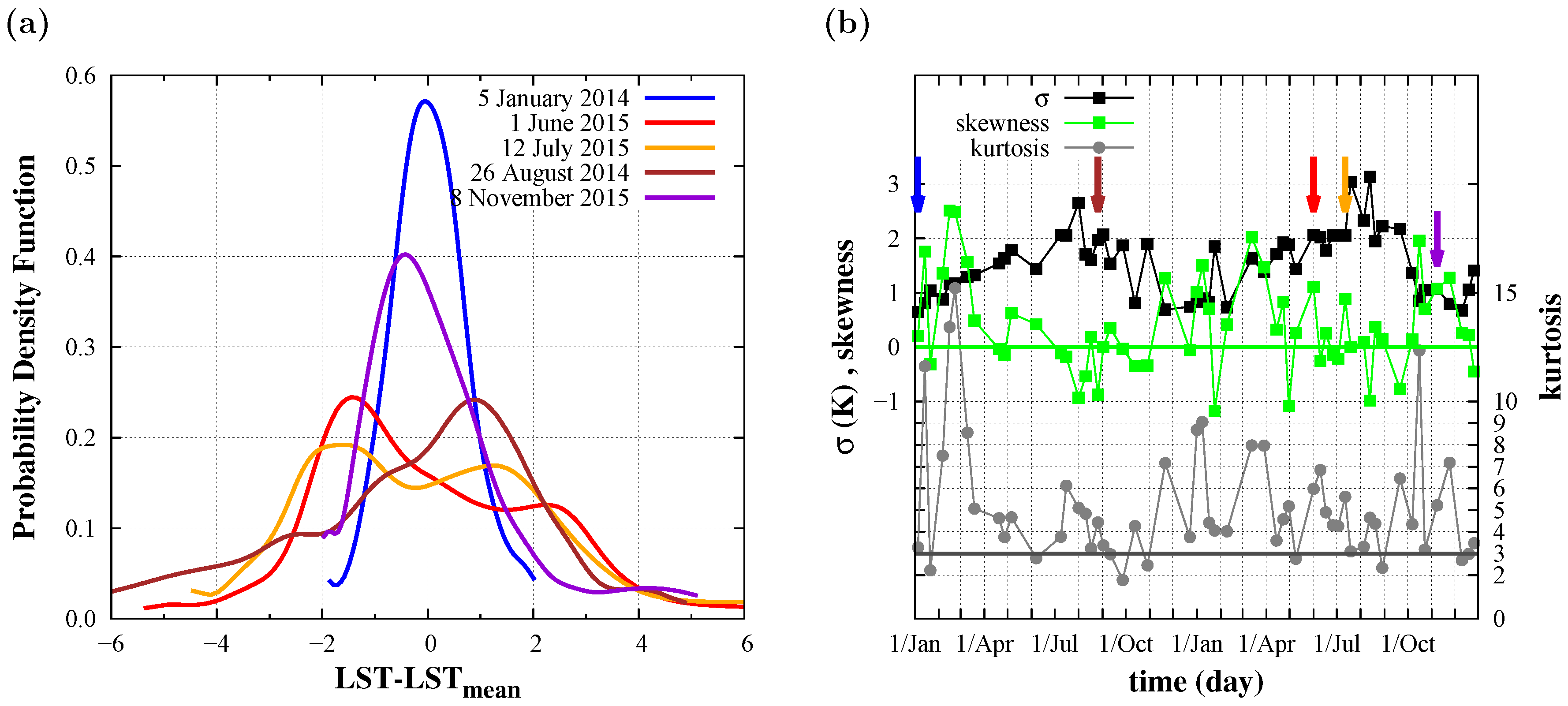
3.3. Seasonal Distribution of LST Heterogeneities

To further explore the heterogeneity of the Landsat 7 ETM+ LST fields during the studied period at the UIB Campus, the corresponding Probability Density Functions (PDFs) are computed as it was done in [46]. Figure 5a shows the PDFs for some selected days that are taken to be representative of the cold seasons (5 January 2014 and 8 November 2015 corresponding to the field in Figure 2c) and the warm ones (1 June 2014, 12 July 2014 and 26 August 2015). The x-axis is normalized by the mean value to make all of these PDFs comparable. In addition, the temporal evolution of the statistical parameters extracted from the PDFs (standard deviation σ, skewness S, and kurtosis K) are shown in Figure 5b for all the available images.
Figure 2c (8 November 2015) shows the variability of the LST field, with the warmest and coldest areas constrained to some specific locations on the Campus. This variability is illustrated by the PDF in Figure 5a that indicates that temperatures lower than average occupy a larger area than the more intense warmer ones. In addition, in agreement with Figure 4, it is seen for this case that the spread of LST for the UIB Campus is smaller than in the warm seasons. The statistics of this distribution (LST m e a n = 294.8 K, σ = 1.1 K, S = 1.1 and K = 5.2) show that it is far from the normal distribution (S = 0, K = 3).
It is clear that the use of PDF illustrates in a compact manner the characteristics of the LST field for the area under study (Figure 5b). For cold season days, such as 5 January 2014, there is a small spread and a distribution very close to the normal one. During the warm season, the distribution shows indication of bi-modality, the maximum evolving during the summer from the cold to the warm side, therefore departing largely from normality. This shift may be related to the progressive drying of the surface during summer, which reduces the areas on the Campus able to be refreshed by evapotranspiration.

4. Conclusions

A satellite-derived LST field provides one value of temperature for each pixel. In this study, the MODIS LST values at a resolution of 1 km—for the area corresponding to the UIB Campus—have been compared to the average values as computed from the available Landsat 7 ETM+ data which are at an approximate resolution of 60 m. The comparative analysis shows that, for the very heterogeneous UIB Campus, the variability at scales under 1 km is very large, the range of LST being on the order of 5–10 K in the winter time and as high as 20 K in the summertime, with standard deviations of about 2 K.
Heterogeneity has an impact on the choice of a position for a station providing ground information. Locating the station arbitrarily in an heterogeneous area may result in a large bias compared to the pixel average if the values at that location are far from the average, compromising even the concept of ground truth validation. The computations made in this work show that the RMSE between in situ LST measurements and MODIS values for the pixel are significantly larger than for homogeneous surfaces, in good correspondence with previous studies. For the Landsat 7 higher resolution pixels, the comparison between in situ and satellite-derived LST compares well for the rather homogeneous area surrounding the station, according to previous studies over homogeneous surfaces.
The analysis of the PDFs of LST from Landsat 7 ETM+ allow inspection of the distribution depending on the time of year for the mid-morning images. The winter time has a more compact distribution as it shows a small spread and a shape closer to normal, whereas the summer time indicates a tendency to bi-modality, the mode moving from cold to warm as summer advances. These distributions may be linked to the contents of water in the soil-vegetation system, since evapotranspiration reduces surface heating wherever it takes place, and, if there is water availability in the whole pixel, heterogeneities may reduce substantially. This effect may reduce its importance as the summer progresses and the land becomes dry.
This prospective work indicates that evaluating the subpixel-scale variability is an important issue, and that it should be considered when using LST in applications over complex heterogeneous terrain. The continuation plans concerning this subject are to install supplementary stations at points representing different surface conditions within the campus and to provide more validation points. The use of TIR onboard a drone flying at low altitude is also envisaged.

Acknowledgments

A. López and B. Martí are acknowledged for their help in field work. This work was funded through the projects CGL2012-37416-C04-01, CGL2013-46862-C2-1-P, CGL2015-65627-C3-1-R and CGL2015-64268-R of the Spanish Government, supplied by the European Regional Development Fund (FEDER). This study was supported by the Conselleria d’Educació, Cultura i Esport of Generalitat Valenciana under the “VALi+D” APOSTD/2015/033 postdoctoral contract and the project PROMETEOII/2014/086 of the Government of Generalitat Valenciana, and the post-doctoral contract of the Spanish Governement BES-2013-065290. Landsat 7 ETM+ and Terra MODIS scenes were freely downloaded from web-tools glovis.usgs.gov and reverb.echo.nasa.gov, respectively.

Author Contributions

This is a prospective paper to orient further investigations. All authors have been involved in the discussions and participated in the writing of the manuscript. The specific contributions of each author in the paper are listed. G. Simó has generated LST from the four-component radiometers and analyzed them against satellite data. V. García-Santos processed the data from the satellites to obtain LST data and computed correlations. M.A. Jiménez computed the PDFs and the derived statistics and generated most of the figures. D. Martínez-Villagrasa has provided quality-controlled data from the reference station. R. Picos has contributed to the discussion and has provided insight into the next steps to be taken. V. Caselles has provided scientific counseling. J. Cuxart provided the scientific direction, defined the structure of the manuscript, and edited it extensively.

Conflicts of Interest

The authors declare no conflict of interest.

References

  1. Jin, M.; Dickinson, R.E. Land surface skin temperature climatology: Benefitting from the strengths of satellite observations. Environ. Res. Lett. 2010, 5, 041002. [Google Scholar] [CrossRef]
  2. Jin, M.; Dickinson, R.E.; Vogelmann, A.M. A comparison of CCM2-BATS skin temperature and surface-air temperature with satellite and surface observations. J. Clim. 1997, 10, 1505–1524. [Google Scholar] [CrossRef]
  3. Popiel, C.O.; Wojtkowiak, J.; Biernacka, B. Measurements of temperature distribution in ground. Exp. Therm. Fluid Sci. 2001, 25, 301–309. [Google Scholar] [CrossRef]
  4. Anderson, M.C.; Allen, R.G.; Morse, A.; Kustas, W.P. Use of Landsat thermal imagery in monitoring evapotranspiration and managing water resources. Remote Sens. Environ. 2012, 122, 50–65. [Google Scholar] [CrossRef]
  5. Kalma, J.D.; McVicar, T.R.; McCabe, M.F. Estimating land surface evaporation: A review of methods using remotely sensed surface temperature data. Surv. Geophys. 2008, 29, 421–469. [Google Scholar] [CrossRef]
  6. Li, Z.L.; Tang, B.H.; Wu, H.; Ren, H.; Yan, G.; Wan, Z.; Trigo, I.F.; Sobrino, J.A. Satellite-derived Land Surface Temperature: Current status and perspectives. Remote Sens. Environ. 2013, 131, 14–37. [Google Scholar] [CrossRef]
  7. Sellers, P.J.; Dickinson, R.E.; Randall, D.A.; Betts, A.K.; Hall, F.G.; Berry, J.A.; Collatz, G.J.; Denning, A.S.; Mooney, H.A.; Nobre, C.A.; et al. Modeling the exchanges of energy, water, and carbon between continents and the atmosphere. Science 1997, 275, 502–509. [Google Scholar] [CrossRef] [PubMed]
  8. Tierney, J.E.; Russell, J.M.; Huang, Y.; Damsté, J.S.S.; Hopmans, E.C.; Cohen, A.S. Northern hemisphere controls on tropical southeast African climate during the past 60,000 years. Science 2008, 322, 252–255. [Google Scholar] [CrossRef] [PubMed]
  9. Cuxart, J.; Conangla, L.; Jiménez, M.A. Evaluation of the surface energy budget equation with experimental data and the ECMWF model in the Ebro Valley. J. Geophys. Res. Atmos. 2015, 120, 1008–1022. [Google Scholar] [CrossRef]
  10. Betts, A.K.; Ball, J.H.; Beljaars, A.C.M.; Miller, M.J.; Viterbo, P.A. The land surface-atmosphere interaction: A review based on observational and global modeling perspectives. J. Geophys. Res. Atmos. 1996, 101, 7209–7225. [Google Scholar] [CrossRef]
  11. Cuxart, J.; Wrenger, B.; Martínez-Villagrasa, D.; Reuder, J.; Jonassen, M.O.; Jiménez, M.A.; Lothon, M.; Lohou, F.; Hartogensis, O.; Dünnermann, J.; et al. Estimation of the advection effects induced by surface heterogeneities in the surface energy budget. Atmos. Chem. Phys. 2016, 14, 9489–9504. [Google Scholar] [CrossRef] [Green Version]
  12. Zhou, J.; Zhang, X.; Zhan, W.; Zhang, H. Land Surface Temperature retrieval from MODIS data by integrating regression models and the genetic algorithm in an arid region. Remote Sens. 2014, 6, 5344–5367. [Google Scholar] [CrossRef]
  13. Niclòs, R.; Valiente, J.A.; Barberà, M.J.; Coll, C. An autonomous system to take angular thermal-infrared measurements for validating satellite products. Remote Sens. 2015, 7, 15269–15294. [Google Scholar] [CrossRef]
  14. Ermida, S.L.; Trigo, I.F.; DaCamara, C.C.; Göttsche, F.M.; Olesen, F.S.; Hulley, G. Validation of remotely sensed surface temperature over an oak woodland landscape—The problem of viewing and illumination geometries. Remote Sens. Environ. 2014, 148, 16–27. [Google Scholar] [CrossRef]
  15. Coll, C.; García-Santos, V.; Niclòs, R.; Caselles, V. Test of the MODIS Land Surface Temperature and emissivity separation algorithm with ground measurements over a rice paddy. IEEE Trans. Geosci. Remote Sens. 2016, 54, 3061–3069. [Google Scholar] [CrossRef]
  16. Krishnan, P.; Kochendorfer, J.; Dumas, E.J.; Guillevic, P.C.; Baker, C.B.; Meyers, T.P.; Martos, B. Comparison of in-situ, aircraft, and satellite land surface temperature measurements over a NOAA climate reference network site. Remote Sens. Environ. 2015, 165, 249–264. [Google Scholar] [CrossRef]
  17. Coll, C.; Galve, J.M.; Sánchez, J.M.; Caselles, V. Validation of Landsat-7/ETM+ thermal-band calibration and atmospheric correction with ground-based measurements. IEEE Transa. Geosci. Remote Sens. 2010, 48, 547–555. [Google Scholar] [CrossRef]
  18. Li, F.; Jackson, T.J.; Kustas, W.P.; Schmugge, T.J.; French, A.N.; Cosh, M.H.; Bindlish, R. Deriving Land Surface Temperature from Landsat 5 and 7 during SMEX02/SMACEX. Remote Sens. Environ. 2004, 92, 521–534. [Google Scholar] [CrossRef]
  19. Mukherjee, S.; Joshi, P.K.; Garg, R.D. Evaluation of LST downscaling algorithms on seasonal thermal data in humid subtropical regions of India. Int. J. Remote Sens. 2015, 36, 2503–2523. [Google Scholar]
  20. Wu, P.; Shen, H.; Zhang, L.; Göttsche, F.M. Integrated fusion of multi-scale polar-orbiting and geostationary satellite observations for the mapping of high spatial and temporal resolution Land Surface Temperature. Remote Sens. Environ. 2015, 156, 169–181. [Google Scholar] [CrossRef]
  21. Weng, Q.; Fu, P.; Gao, F. Generating daily Land Surface Temperature at Landsat resolution by fusing Landsat and MODIS data. Remote Sens. Environ. 2014, 145, 55–67. [Google Scholar] [CrossRef]
  22. Yu, W.; Ma, M. Scale mismatch between in situ and remote sensing observations of Land Surface Temperature: Implications for the validation of remote sensing LST products. IEEE Geosci. Remote Sens. Lett. 2015, 12, 497–501. [Google Scholar]
  23. Jiménez, M.A.; Mira, A.; Cuxart, J.; Luque, A.; Alonso, S.; Guijarro, J.A. Verification of a clear-sky mesoscale simulation using satellite-derived surface temperatures. Mon. Weather Rev. 2008, 136, 5148–5161. [Google Scholar] [CrossRef]
  24. Jiménez, M.A.; Ruiz, A.; Cuxart, J. Estimation of cold pool areas and chilling hours through satellite-derived surface temperatures. Agric. For. Meteorol. 2015, 207, 58–68. [Google Scholar] [CrossRef]
  25. Cuxart, J.; Jiménez, M.A.; Martínez, D. Nocturnal meso-beta basin and katabatic flowson a midlatitude island. Mon. Weather Rev. 2007, 135, 918–932. [Google Scholar] [CrossRef]
  26. Cuxart, J.; Jiménez, M.A.; Telisman-Prtenjak, M.; Grisogono, B. Study of a sea-breeze case through momentum, temperature, and turbulence budgets. J. Appl. Meteorol. Climatol. 2014, 53, 2589–2609. [Google Scholar] [CrossRef]
  27. Hook, S.J.; Gabell, A.R.; Green, A.A.; Kealy, P.S. A comparison of techniques for extracting emissivity information from thermal infrared data for geologic studies. Remote Sens. Environ. 1992, 42, 123–135. [Google Scholar] [CrossRef]
  28. Landsat 7 Science Data Users Handbook. Technical Report; U.S. Geological Survey, 1998. Available online: http://landsathandbook.gsfc.nasa.gov (accessed on 1 August 2016).
  29. Hulley, G.C.; Hook, S.J.; Abbott, E.; Malakar, N.; Islam, T.; Abrams, M. The ASTER Global Emissivity Dataset (ASTER GED): Mapping Earth’s emissivity at 100 m spatial scale. Geophys. Res. Lett. 2015, 42, 7966–7976. [Google Scholar] [CrossRef]
  30. Yamaguchi, Y.; Kahle, A.B.; Tsu, H.; Kawakami, T.; Pniel, M. Overview of advanced spaceborne thermal emission and reflection radiometer (ASTER). IEEE Trans. Geosci. Remote Sens. 1998, 36, 1062–1071. [Google Scholar] [CrossRef]
  31. Gillespie, A.; Rokugawa, S.; Matsunaga, T.; Cothern, C.J.; Hook, S.; Kahle, A.B. A temperature and emissivity separation algorithm for Advanced Spaceborne Thermal Emission and Reflection Radiometer (ASTER) images. IEEE Trans. Geosci. Remote Sens. 1998, 36, 1113–1126. [Google Scholar] [CrossRef]
  32. Berk, A.; Anderson, G.P.; Acharya, P.K.; Bernstein, L.S.; Muratov, L.; Lee, J.; Fox, M.; Adler-Golden, S.M.; Chetwynd, J.H., Jr.; Hoke, M.L.; et al. MODTRAN5: 2006 update. Proc. SPIE 2006. [Google Scholar] [CrossRef]
  33. Barsi, J.A.; Schott, J.R.; Palluconi, F.D.; Hook, S.J. Validation of a web-based atmospheric correction tool for single thermal band instruments. Proc. SPIE 2005. [Google Scholar] [CrossRef]
  34. Pérez-Planells, L.; García-Santos, V.; Caselles, V. Comparing different profiles to characterize the atmosphere for three MODIS TIR bands. Atmos. Res. 2015, 161–162, 108–115. [Google Scholar] [CrossRef]
  35. Wan, Z.; Dozier, J. A generalised split-window algorithm for retrieving land-surface temperature from space. IEEE Trans. Geosci. Remote Sens. 1996, 34, 892–905. [Google Scholar]
  36. Wan, Z.; Li, Z.L. A physics-based algorithm for retrieving land-surface emissivity and temperature from EOS/MODIS data. IEEE Trans. Geosci. Remote Sens. 1997, 35, 980–996. [Google Scholar]
  37. Hulley, G.; Hook, S.; Hughes, C. MODIS MOD21 Land Surface Temperature and Emissivity Algorithm Theoretical Basis Document; Jet Propulsion Laboratory Publications: Pasadena, CA, USA, 2012. [Google Scholar]
  38. Tonooka, H. Accurate atmospheric correction of ASTER thermal infrared imagery using the WVS method. IEEE Trans. Geosci. Remote Sens. 2005, 43, 2778–2792. [Google Scholar] [CrossRef]
  39. Wan, Z.; Zhang, Y.; Zhang, Y.Q.; Li, Z.L. Validation of the Land Surface Temperature products retrieved from Moderate Resolution Imaging Spectroradiometer data. Remote Sens. Environ. 2002, 83, 163–180. [Google Scholar] [CrossRef]
  40. Hook, S.J.; Vaughan, R.G.; Tonooka, H. Absolute radiometric in-flight validation of mid infrared and thermal infrared data from ASTER and MODIS on the Terra spacecraft using the Lake Tahoe, CA/NV, USA, Automated Validation Site. IEEE Trans. Geosci. Remote Sens. 2007, 45, 1798–1807. [Google Scholar] [CrossRef]
  41. Coll, C.; Wan, Z.; Galve, J.M. Temperature-based and radiance-based validations of the V5 MODIS Land Surface Temperature product. J. Geophys. Res. 2009, 114, 1–15. [Google Scholar] [CrossRef]
  42. Hulley, G.C.; Hook, S.J. Intercomparison of Versions 4, 4.1 and 5 of the MODIS land surface temperature and emissivity products and validation with laboratory measurements of sand samples from the Namib Desert, Namibia. Remote Sens. Environ. 2009, 113, 1313–1318. [Google Scholar] [CrossRef]
  43. Wan, Z. New refinements and validation of the MODIS Land-Surface Temperature/Emissivity products. Remote Sens. Environ. 2008, 112, 59–74. [Google Scholar] [CrossRef]
  44. Snyder, W.C.; Wan, Z.; Zhang, Y.; Feng, Y.Z. Classification-based emissivity for Land Surface Temperature measurement from space. J. Remote Sens. 1998, 19, 2753–2774. [Google Scholar] [CrossRef]
  45. Vlassova, L.; Perez-Cabello, F.; Nieto, H.; Martín, P.; Riano, D.; de la Riva, J. Assessment of methods for Land Surface Temperature retrieval from Landsat-5 TM images applicable to multiscale tree-grass ecosystem modeling. Remote Sens. 2014, 6, 4345–4368. [Google Scholar] [CrossRef]
  46. Jiménez, M.A.; Cuxart, J. Study of the probability density functions from a large-eddy simulation for a stably stratified boundary layer. Bound. Layer Meteorol. 2006, 118, 401–420. [Google Scholar] [CrossRef]
Figure 1. (a) topography of the island of Mallorca (Balearic Islands, Western Mediterranean Sea) with the location of the Campus of the Universitat de les Illes Balears (UIB) and in (b) a zoom over it. The yellow dot indicates the location of the complete energy balance station and the red dots other locations that are further explored in this work.
Remotesensing 08 00849 g001
Figure 2. (a) Red, Green, Blue (RGB) image obtained on 8 November 2015 at 10:30 UTC for the study area and its surroundings from Landsat 7. Yellow, purple, red and green squares correspond to the pixels of Moderate Resolution Imaging Spectroradiometer (MODIS). The corresponding Advanced Spaceborne Thermal Emission and Reflection Radiometer (ASTER) emissivity (bands 13 and 14) and LST for Landsat 7 and MODIS are shown in (bd), respectively. The white square is the 1 km 2 studied area at the UIB Campus (Figure 1b) and white dots indicate the location of the selected points further analyzed. M1, M2, M3 and M4 indicate the location of the MODIS pixels that fall within the study area.
Remotesensing 08 00849 g002
Figure 3. (a) time series of averaged LST over the 1 km 2 studied area in the UIB Campus for Terra MODIS (weighted average) in red and Landsat 7 ETM+ in blue. Data from the meteorological station (see location in Figure 1b, yellow dot) are also included in black empty squares; and (b) the correlation of LST obtained from the three different sources. Here, the Landsat 7 LST corresponds to the closest value when compared to the ground station, and it is the 1 km 2 spatial average when it is compared to MODIS.
Remotesensing 08 00849 g003
Figure 4. Time series of the maximum (in red) and minimum (in blue) LST obtained from Landsat 7 ETM+ for the 1 km 2 studied area at the Campus. LST evolution for the closest Landsat 7 ETM+ pixel is also included from the nine selected points and the energy balance measurement site (see locations in Figure 1b).
Remotesensing 08 00849 g004
Figure 5. (a) normalized probability density functions (PDFs) computed from the Landsat 7 ETM+ LST fields over the UIB Campus for different days within the cold and hot seasons (see figure legend). (b) time series of the standard deviation (σ), skewness and kurtosis of the PDFs computed from the Landsat 7 ETM+ LST fields from 1 January 2014 to 1 January 2016. The arrows indicate the statistical parameters of the PDFs shown in (a).
Remotesensing 08 00849 g005
Table 1. Root Mean Square Error (RMSE) and bias of the differences between the in situ measurements minus the satellite-derived Land-Surface Temperature (LST) (MOD11 from Moderate Resolution Imaging Spectroradiometer (MODIS) and ETM+ from Landsat 7). The last rows for MODIS and ETM+ show results from the current work. For each comparison, a brief description of the surface site and the radiometer type is given: bold in the surface type column refers to heterogeneous sites; ground measurements computed as an average from different point measurements are indicated in bold in the radiometer column and, in brackets, the number of devices used. Statistics are computed from both day and nighttime cases together. In brackets, the results are obtained only considering the daytime cases. ( * ) indicates that the statistics refer to the robust RMSE and Median, providing very similar results to the corresponding RMSE and bias according to [15]. The study from [22] shows the percentage of cases that fall into different absolute bias ranges, distinguishing nighttime results in square brackets. [cw] = current work.
SensorSurface TypeRadiometerRMSE (K)Bias (K)Referenece
MODISBare soil8–14 μm broadband (×1, handheld)1.1[12]
Shrubland8–14 μm broadband (×1)2.70.8[13]
Rice crop1.80.1
Oak woodlan8–14 μm broadband (×3)2.4
(3.2)
1.5
(2.7)
[14]
Seed corn, roads and buildings8–14 μm broadband (×7)(15%) [53%] < 1 K
(42%) > 3 K
[22]
5–50 μm 4 component (×1)(33%) [57%] < 1 K
(15%) > 3 K
Rice cropmultispectral (×4)
8–14 μm broadband (×2)
0.6 *0.1 *[15]
Grassland and hardwood deciduous forest 8–14 μm broadband (×3)2.8
(3.1)
0.6
(1.8)
[16]
Grassland, crops, asphalt, wet regions5–50 μm 4 component (×1)(4.2)(3.2)[cw]
ETM+Rice cropmultispectral (×3)(1.1)0[17]
Soybean and corn crops8–14 μm broadband (×12)(1.2)[18]
Grassland, crops, asphalt, wet regions5–50 μm 4 component (×1)(1.7)(−0.5)[cw]

