
Random Forest Classification of Wetland Landcovers from Multi-Sensor Data in the Arid Region of Xinjiang, China

Abstract
:
1. Introduction
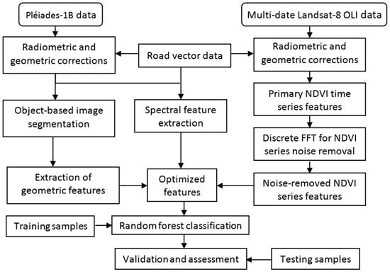
2. Data and Methods
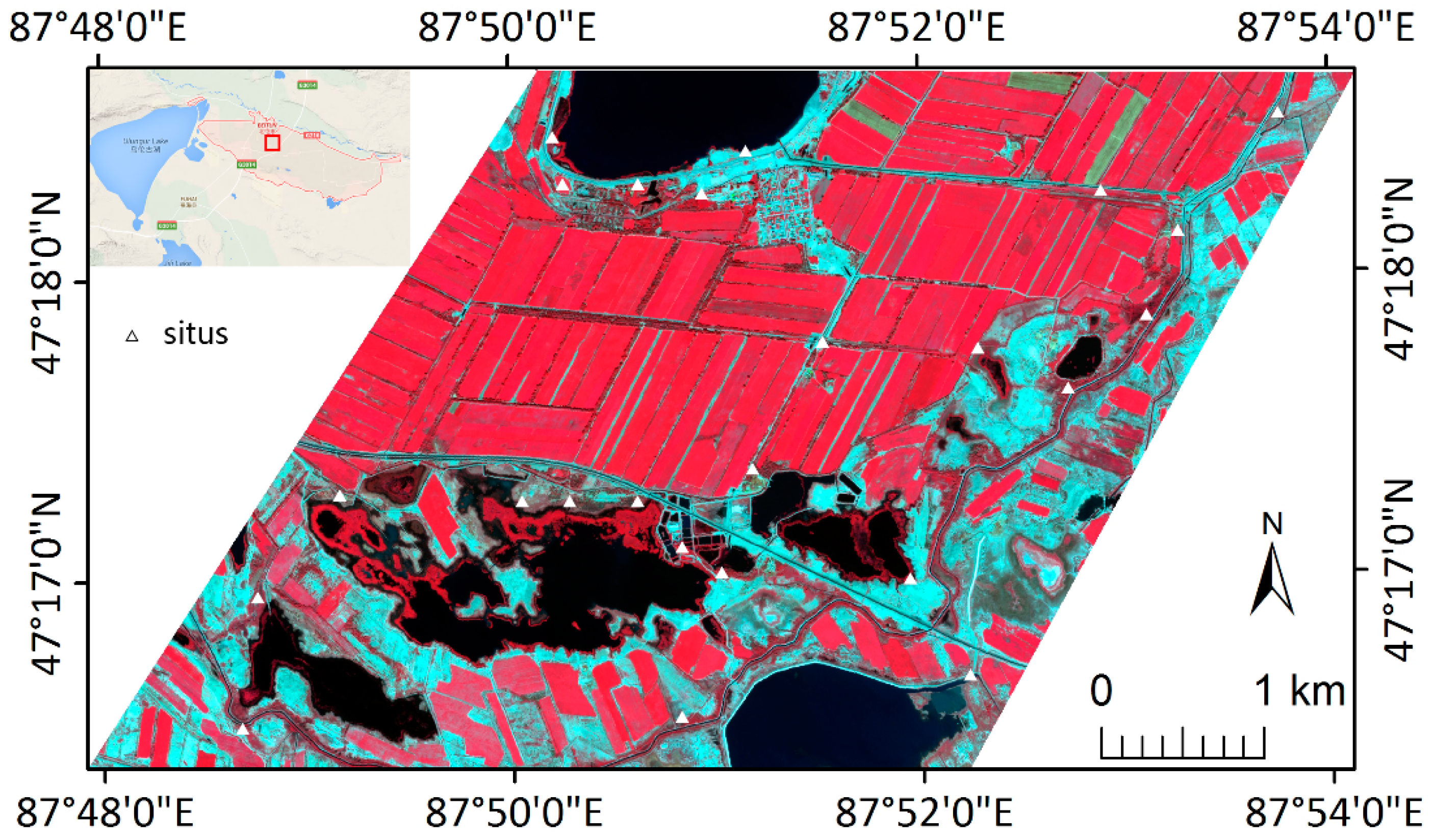
2.1. Study Area and Data Acquisition
2.1.1. Study Area
2.1.2. Data Acquisition and Preprocessing
Pléiades-1B Multispectral Data
Calculation of Landsat-8 Normalized Difference Vegetation Index (NDVI)
2.2. Random Forest Classifier
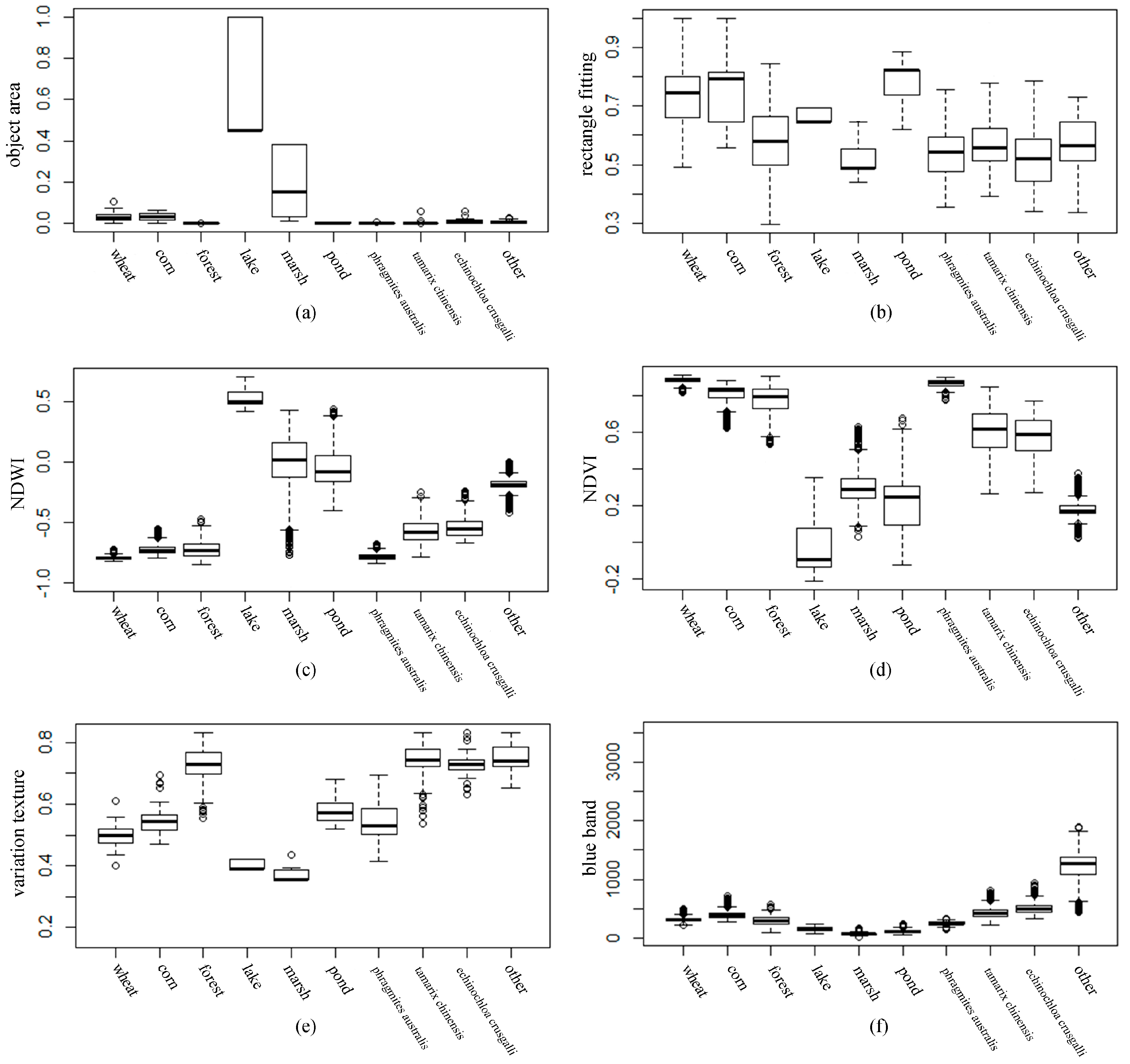
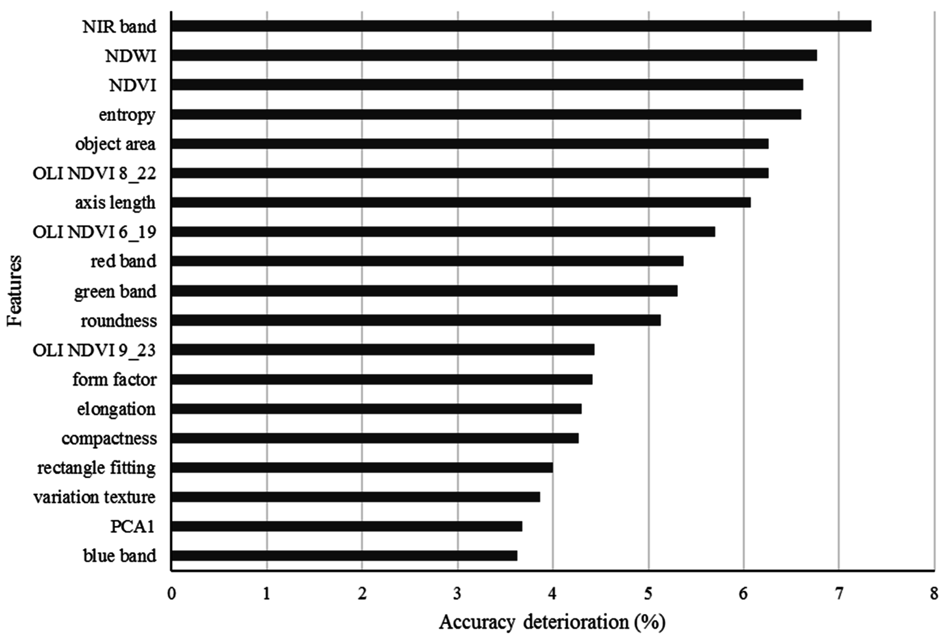
2.3. Feature Extraction and Optimization
2.3.1. Spectral Feature Selection and Optimization
2.3.2. Object-Oriented Feature Extraction
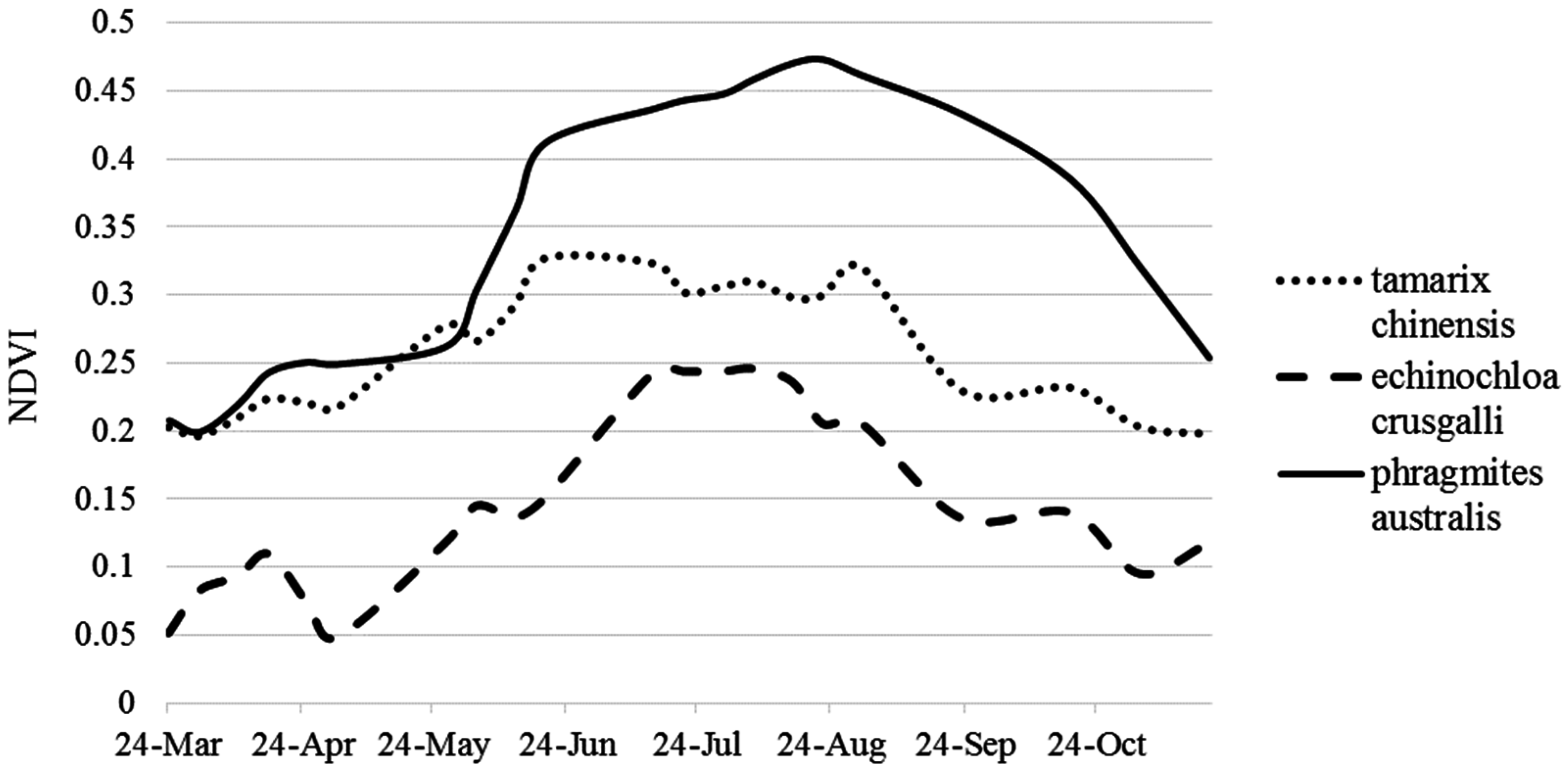
2.3.3. Calculation of the NDVI Series
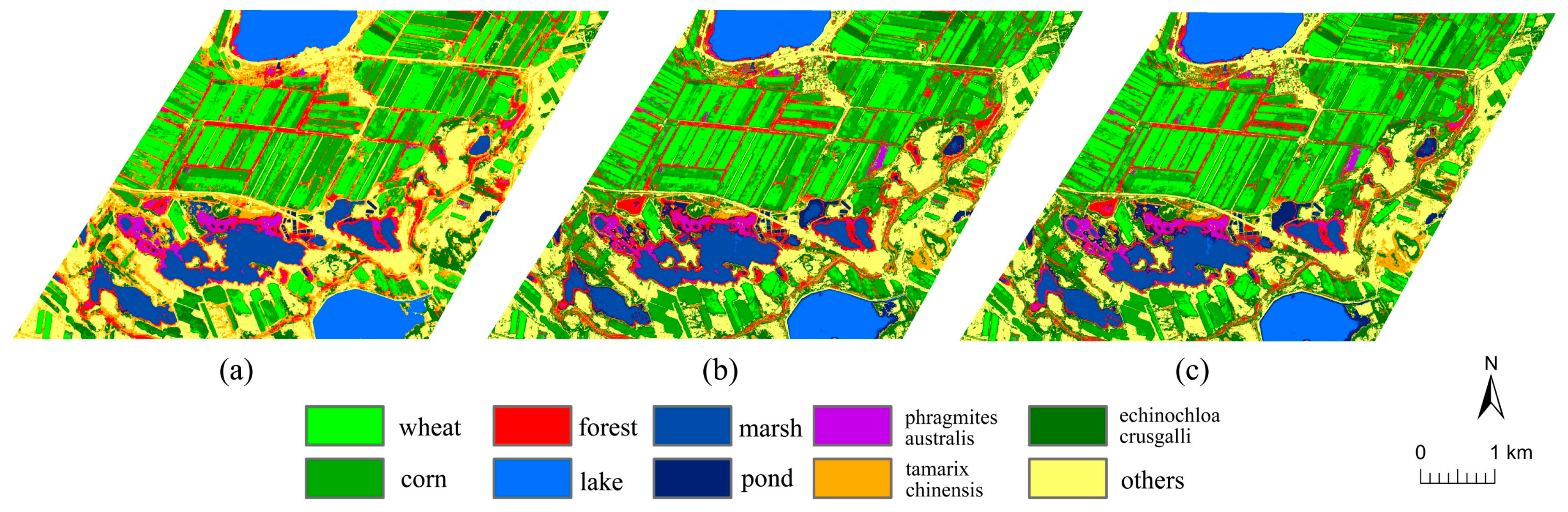
3. Experiment and Results
4. Discussion
5. Conclusions
Acknowledgments
Author Contributions
Conflicts of Interest
References
- Tong, L.; Xu, X.; Fu, Y.; Li, S. Wetland changes and their responsest climate change in the “three-river headwaters” region of China since the 1990s. Energies 2014, 7, 2515–2534. [Google Scholar] [CrossRef]
- Jiang, P.; Cheng, L.; Li, M.; Zhao, R.; Huang, Q. Analysis of landscape fragmentation processes and driving forces in wetlands in arid areas: A case study of the middle reaches of the Heihe River, China. Ecol. Indic. 2014, 46, 240–252. [Google Scholar] [CrossRef]
- Turpie, K.R.; Klemas, V.V.; Byrd, K.; Kelly, M.; Jo, Y.-H. Prospective HyspIRI global observations of tidal wetlands. Remote Sens. Environ. 2015, 167, 206–217. [Google Scholar] [CrossRef]
- Rapinel, S.; Hubert-Moy, L.; Clément, B. Combined use of LiDAR data and multispectral earth observation imagery for wetland habitat mapping. Int. J. Appl. Earth Obs. Geoinf. 2015, 37, 56–64. [Google Scholar] [CrossRef]
- Kloiber, S.M.; Macleod, R.D.; Smith, A.J.; Knight, J.F.; Huberty, B.J. A semi-automated, multi-source data fusion update of a wetland inventory for east-central Minnesota, USA. Wetlands 2015, 35, 335–348. [Google Scholar] [CrossRef]
- Martínez-López, J.; Carreño, M.F.; Palazón-Ferrando, J.A.; Martínez-Fernández, J.; Esteve, M.A. Remote sensing of plant communities as a tool for assessing the condition of semiarid Mediterranean saline wetlands in agricultural catchments. Int. J. Appl. Earth Obs. Geoinf. 2014, 26, 193–204. [Google Scholar] [CrossRef]
- Thakur, J.K.; Srivastava, P.K.; Singh, S.K.; Vekerdy, Z. Ecological monitoring of wetlands in semiarid region of Konya closed Basin Turkey. Reg. Environ. Chang. 2012, 12, 133–144. [Google Scholar] [CrossRef]
- Davranche, A.; Lefebvre, G.; Poulin, B. Wetland monitoring using classification trees and SPOT-5 seasonal time series. Remote Sens. Environ. 2010, 114, 552–562. [Google Scholar] [CrossRef] [Green Version]
- Huang, C.; Peng, Y.; Lang, M.; Yeo, I.-Y.; McCarty, G. Wetland inundation mapping and change monitoring using Landsat and airborne LiDAR data. Remote Sens. Environ. 2014, 141, 231–242. [Google Scholar] [CrossRef]
- Hong, S.; Jang, H.; Kim, N.; Sohn, H. Water area extraction using RADARSAT SAR imagery combined with Landsat imagery and terrain information. Sensors 2015, 15, 6652–6667. [Google Scholar] [CrossRef] [PubMed]
- Hess, L.L.; Melack, J.M.; Affonso, A.G.; Barbosa, C.; Gastil-Buhl, M.; Novo, E.M.L.M. Wetlands of lowland Amazon basin: Extent, Vegetative Cover, and dual-season inundated area as mapped with JERS-1 Synthetic Aperture Rader. Wetlands 2015, 35, 745–756. [Google Scholar] [CrossRef]
- Chen, Y.; He, X.; Wang, J. Classification of coastal wetlands in eastern China using polarimetric SAR data. Arab. J. Geosci. 2015, 8, 10203–10211. [Google Scholar] [CrossRef]
- Han, X.; Chen, X.; Feng, L. Four decades of winter wetland changes in Poyang Lake based on Landsat observations between 1973 and 2013. Remote Sens. Environ. 2015, 156, 426–437. [Google Scholar] [CrossRef]
- Zhang, S.; Zhang, C.; Zhang, L.; Zhang, Y. Wetland Remote sensing classification using support vector machine optimized with genetic algorithm: A case study in Honghe Nature National Reserve. Sci. Geogr. Sin. 2012, 32, 435–441. [Google Scholar]
- Liu, L.; Zang, S.; Na, X.; Pei, X. Wetland mapping in Zhalong Natural Reserve using optical and radar remotely sensed data and ancillary topographical data. Geogr. Geo-Inf. Sci. 2013, 29, 36–40. [Google Scholar]
- Wright, C.; Gallant, A. Improved wetland remote sensing in Yellowstone National Park using classification trees to combine TM imagery and ancillary environmental data. Remote Sens. Environ. 2007, 107, 582–605. [Google Scholar] [CrossRef]
- Torbick, N.; Salas, W. Mapping agricultural wetlands in the Sacramento Valley, USA with satellite remote sensing. Wetl. Ecol. Manag. 2015, 23, 79–94. [Google Scholar] [CrossRef]
- Macalister, C.; Mahaxay, M. Mapping wetlands in the Lower Mekong Basin for wetland resource and conservation management using Landsat ETM images and field survey data. J. Environ. Manag. 2009, 90, 2130–2137. [Google Scholar] [CrossRef] [PubMed]
- Kumar, A.L.; Sinha, P.; Taylor, S. Improving image classification in a complex wetland ecosystem through image fusion techniques. J. Appl. Remote Sens. 2014, 8, 4480–4494. [Google Scholar] [CrossRef]
- Bao, Y.; Ren, J. Wetland Landscape Classification Based on the BP neural network in DaLinor Lake area. Procedia Environ. Sci. 2011, 10, 2360–2366. [Google Scholar] [CrossRef]
- Augusteijn, M.F.; Warrender, C.E. Wetland classification using optical and radar data and neural network classification. Int. J. Remote Sens. 1998, 19, 1545–1560. [Google Scholar] [CrossRef]
- Laba, M.; Blair, B.; Downs, R.; Monger, B.; Philpot, W.; Smith, S.; Sullivan, P.; Baveye, P.C. Use of textural measurements to map invasive wetland plants in the Hudson River National Estuarine Research Reserve with IKONOS satellite imagery. Remote Sens. Environ. 2010, 114, 876–886. [Google Scholar] [CrossRef]
- Dronova, I.; Gong, P.; Wang, L.; Zhong, L. Mapping dynamic cover types in a large seasonally flooded wetland using extended principal component analysis and object-based classification. Remote Sens. Environ. 2015, 158, 193–206. [Google Scholar] [CrossRef]
- Dronova, I.; Gong, P.; Wang, L. Object-based analysis and change detection of major wetland cover types and their classification uncertainty during the low water period at Poyang Lake, China. Remote Sens. Environ. 2011, 115, 3220–3236. [Google Scholar] [CrossRef]
- Lane, C.; Liu, H.; Autrey, B.; Anenkhonov, O.A.; Chepinoga, V.V.; Wu, Q. Improved wetland classification using eight-band high resolution satellite imagery and a hybrid approach. Remote Sens. 2014, 6, 12187–12216. [Google Scholar] [CrossRef]
- Collins, S.D.; Heintzman, L.J.; Starr, S.M.; Wright, C.K.; Henebry, G.M.; Mclntyre, N.E. Hydrological dynamics of temporary wetlands in the southern Great Plains as a function of surrounding land use. J. Arid Environ. 2014, 109, 6–14. [Google Scholar] [CrossRef]
- Breiman, L. Random forests. Mach. Learn. 2001, 45, 5–32. [Google Scholar] [CrossRef]
- Dietterich, T.G. An experimental comparison of three methods for constructing ensembles of decision trees: Bagging, boosting, and randomization. Mach. Learn. 2000, 40, 139–157. [Google Scholar] [CrossRef]
- Corcoran, J.M.; Knight, J.F.; Gallant, A.L. Influence of multi-source and multi-temporal remotely sensed and ancillary data on the accuracy of random forest classification of wetlands in northern Minnesota. Remote Sens. 2013, 5, 3212–3238. [Google Scholar] [CrossRef]
- Millard, K.; Richardson, M. Wetland mapping with LiDAR derivatives, SAR polarimetric decompositions, and LiDAR-SAR fusion using a random forest classifier. Can. J. Remote Sens. 2013, 39, 290–307. [Google Scholar] [CrossRef]
- Stumpf, A.; Kerle, N. Object-oriented mapping of landslides using Random Forests. Remote Sens. Environ. 2011, 115, 2564–2577. [Google Scholar] [CrossRef]
- Gislason, P.O.; Benediktsson, J.A.; Sveinsson, J.R. Random forests for land cover classification. Pattern Recognit. Lett. 2006, 27, 294–300. [Google Scholar] [CrossRef]
- Hayes, M.M.; Miller, S.N.; Murphy, M.A. High-resolution landcover classification using Random Forest. Remote Sens. Lett. 2014, 5, 112–121. [Google Scholar] [CrossRef]
- Zhu, C.; Li, J.; Chang, C.; Luo, J. Remote sensing detection and spatio-temporal change analysis of welands in Xinjiang arid region. Trans. Chin. Soc. Agric. Eng. 2014, 30, 229–238. [Google Scholar]
- Zhang, K.; Li, R.; Liu, Y.; Wang, B.; Yang, X.; Hou, R. Spatial pattern of a plant community in a wetland ecosystem in a semiarid region in northwestern China. Front. For. China 2008, 3, 326–333. [Google Scholar] [CrossRef]
- Ozesmi, S.L.; Bauer, M.E. Satellite remote sensing of wetlands. Wetl. Ecol. Manag. 2002, 10, 381–402. [Google Scholar] [CrossRef]
- Tian, S.; Zhang, X. Random forest classification of land cover information of urban areas in arid regions based on TH-1 data. Remote Sens. Land Resour. 2016, 28, 43–49. [Google Scholar]
- Chan, C.W.; Paelinckx, D. Evaluation of Random Forest and Adaboost tree-based ensemble classification and spectral band selection for ecotope mapping using airborne hyperspectral imagery. Remote Sens. Environ. 2008, 112, 2999–3011. [Google Scholar] [CrossRef]
- Ho, T.K. The random subspace method for constructing decision forests. IEEE Trans. Pattern Anal. Mach. Intell. 1998, 20, 832–844. [Google Scholar]
- Rodriguez-Galiano, V.F.; Ghimire, B.; Rogan, J.; Chica-Olmo, M.; Rigol-Sanchez, J.P. An assessment of the effectiveness of a random forest classifier for land-cover classification. ISPRS J. Photogramm. Remote Sens. 2012, 67, 93–104. [Google Scholar] [CrossRef]
- McFeeters, S.K. The use of Normalized Difference Water Index (NDWI) in the delineation of open water features. Int. J. Remote Sens. 1996, 17, 1425–1432. [Google Scholar] [CrossRef]
- Jenicka, S.; Suruliandi, A. A textural approach for land cover classification of remotely sensed image. CSI Trans. ICT 2014, 2, 1–9. [Google Scholar] [CrossRef]
- Rodriguez-Galiano, V.F.; Chica-Olmo, M.; Abarca-Hernandez, F.; Atkinson, P.M.; Jeganathan, C. Random Forest classification of Mediterranean land cover using multi-seasonal imagery and multi-seasonal texture. Remote Sens. Environ. 2012, 121, 93–107. [Google Scholar] [CrossRef]
- Na, X.; Zhang, S.; Li, X.; Qin, X.W. Application of MODIS NDVI time series to extracting wetland vegetation information in the Sanjiang Plain. Wetl. Sci. 2007, 5, 227–235. [Google Scholar]
- Girma, A.; de Bie, C.A.J.M.; Skidmore, A.K.; Venus, V.; Bongers, F. Hyper-temporal SPOT-NDVI dataset parameterization captures species distributions. Int. J. Geogr. Inf. Sci. 2015, 30, 89–107. [Google Scholar] [CrossRef]
- Zhou, J.; Qin, J.; Gao, K.; Leng, H. SVM-based soft classification of urban tree species using very high-spatial resolution remote-sensing imagery. Int. J. Remote Sens. 2016, 37, 2541–2559. [Google Scholar] [CrossRef]
- Shi, W.; Zhao, Y.; Wang, Q. Sub-pixel mapping based on BP neural network with multiple shifted remote sensing images. J. Infrared Millim. Waves 2014, 33, 527–532. [Google Scholar]


| Level 1 | Level 2 | Level 3 | Level 4 |
|---|---|---|---|
| Non-wetland | Farming land | Arable land | Wheat |
| Farming land | Arable land | Corn | |
| Planted vegetation | Planted trees | Forest | |
| Wetland | Open waters | Freshwater wetland | Lake |
| Marsh | |||
| Pond | |||
| Natural plants | Phragmites australis | ||
| Tamarix chinensis | |||
| Echinochloa crusgalli | |||
| Others | Others |
| Classifier | RFC | SVM | ANN | RFC-Pleiade-1B | RFC-OLI NDVI |
|---|---|---|---|---|---|
| Overall accuracy (%) | 92.5 | 83.3 | 80.2 | 86.7 | 68.9 |
| Kappa coefficient | 0.92 | 0.81 | 0.78 | 0.84 | 0.65 |
| Class | Commission Errors | Omission Errors | Producer’s Accuracy | User’s Accuracy |
|---|---|---|---|---|
| Wheat | 1.42 | 3.38 | 96.62 | 98.58 |
| Corn | 3.38 | 2.79 | 97.21 | 96.62 |
| Forest | 13.39 | 7.84 | 92.16 | 86.61 |
| Lake | 0.00 | 0.00 | 100 | 100 |
| Marsh | 1.36 | 2.11 | 97.89 | 98.64 |
| Pond | 3.72 | 3.47 | 96.53 | 96.28 |
| Phragmites australis | 1.81 | 15.44 | 84.56 | 98.19 |
| Tamarix chinensis | 12.23 | 8.12 | 91.88 | 87.77 |
| Echinochloa crusgalli | 1.78 | 9.97 | 90.03 | 98.72 |
| Others | 4.81 | 0.59 | 99.41 | 95.19 |
© 2016 by the authors; licensee MDPI, Basel, Switzerland. This article is an open access article distributed under the terms and conditions of the Creative Commons Attribution (CC-BY) license (http://creativecommons.org/licenses/by/4.0/).
Share and Cite
Tian, S.; Zhang, X.; Tian, J.; Sun, Q. Random Forest Classification of Wetland Landcovers from Multi-Sensor Data in the Arid Region of Xinjiang, China. Remote Sens. 2016, 8, 954. https://0-doi-org.brum.beds.ac.uk/10.3390/rs8110954
Tian S, Zhang X, Tian J, Sun Q. Random Forest Classification of Wetland Landcovers from Multi-Sensor Data in the Arid Region of Xinjiang, China. Remote Sensing. 2016; 8(11):954. https://0-doi-org.brum.beds.ac.uk/10.3390/rs8110954
Chicago/Turabian StyleTian, Shaohong, Xianfeng Zhang, Jie Tian, and Quan Sun. 2016. "Random Forest Classification of Wetland Landcovers from Multi-Sensor Data in the Arid Region of Xinjiang, China" Remote Sensing 8, no. 11: 954. https://0-doi-org.brum.beds.ac.uk/10.3390/rs8110954