
Evaluation and Improvement of SMOS and SMAP Soil Moisture Products for Soils with High Organic Matter over a Forested Area in Northeast China


Abstract
:1. Introduction
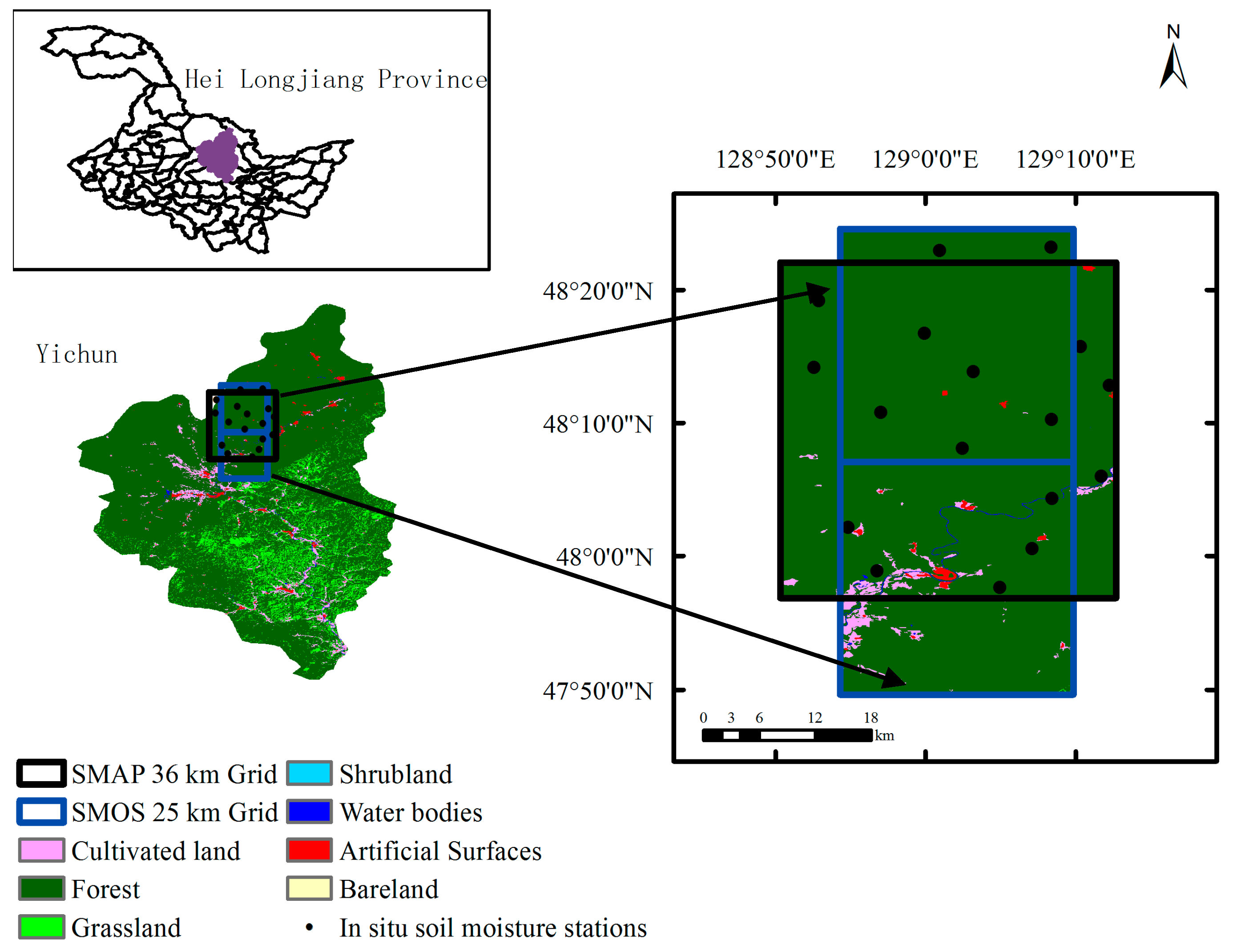
2. Study Area
3. Materials and Methods
3.1. Datasets
3.1.1. The Ground Wireless Sensor Network (GWSN) SM Measurements
3.1.2. SMOS Data
3.1.3. SMAP Data
3.1.4. Additional Data
3.2. Methodology
3.2.1. Methodology for Comparison
3.2.2. Methodology for Obtaining Revised Satellite SM
- (1)
- Obtain the key parameters of the L-MEB model, such as canopy parameters optical depth (τNAD) and albedo (ω), land surface temperature parameter TS, and the four soil roughness parameters QR , HR and NRP (p = H or V) of the model employed by Marie Parrens et al. [15]. For SMOS, τNAD and TS were obtained from the SMOS L3 daily SM products, and ω and HR were assumed to be constant as described in [6], with ω = 0.07 and HR = 1.2. For SMAP, the values of τNAD, ω, TS, and HR were obtained from the SMAP L3 daily SM products. Here, we assumed that NRP = 0 (p = H or V) for both SMOS and SMAP. QR was also approximated to zero as had been done in the SMOS and SMAP retrieval algorithms, since QR was low at L-band [17,37,38].
- (2)
- Run Liu’s model instead of the Mironov model within the L-MEB model to obtain new expressions for TB_Sim for SMOS and SMAP, based on their own L-MEB model parameters.
- (3)
- Minimize the cost function CF (Equation (4)) by a generalized least squares iterative algorithm to achieve the revised SM values. For both SMOS and SMAP, the initial value for SM from the inversion process was the corresponding satellite SM product value. TB_Obs was the corresponding satellite observed brightness temperature value, which was obtained from the SMOS (incident angle approximately 42.5°) and SMAP (incident angle approximately 40°) L3 daily SM products.
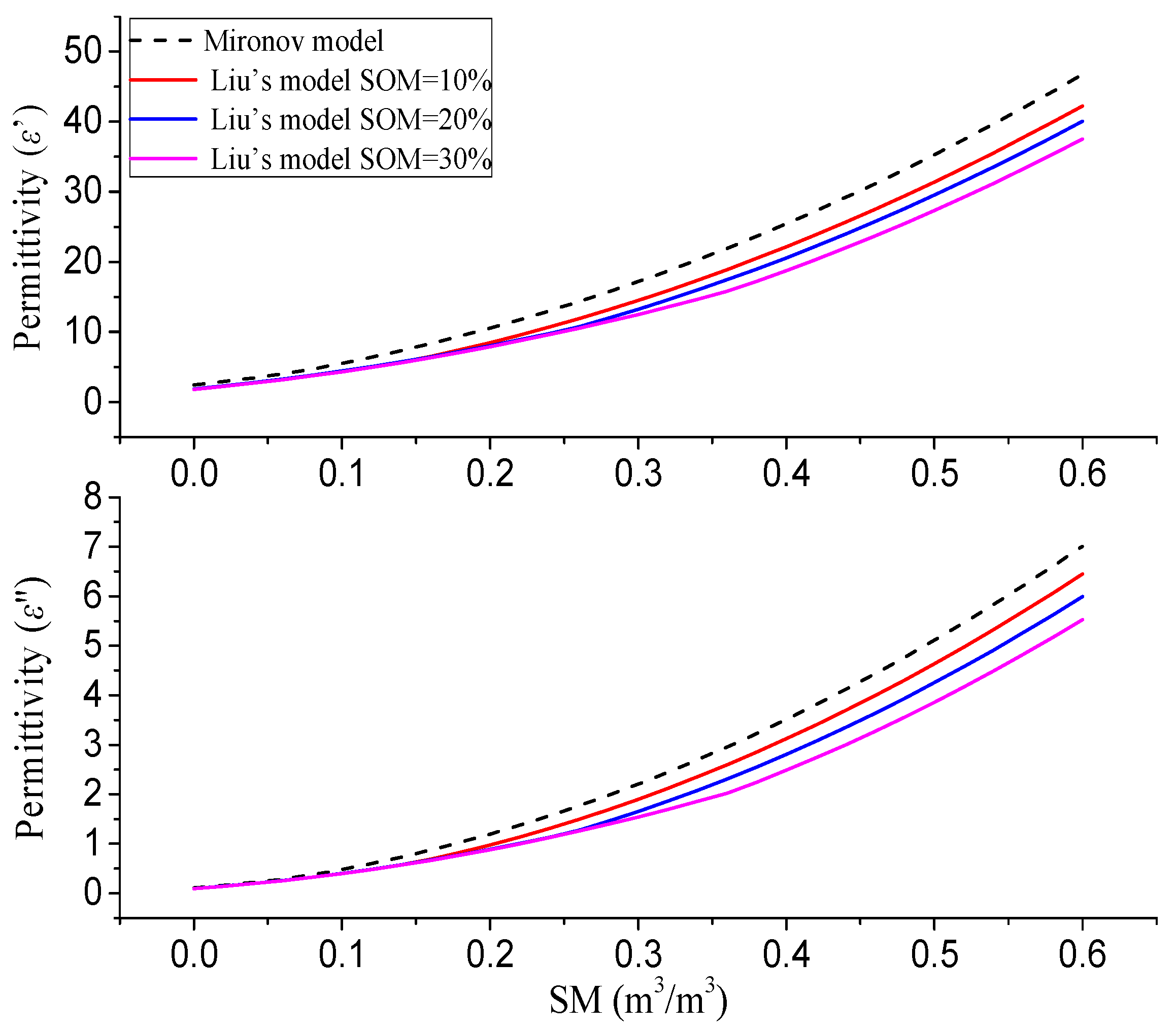
3.2.3. Liu’s Model
4. Results and Discussion
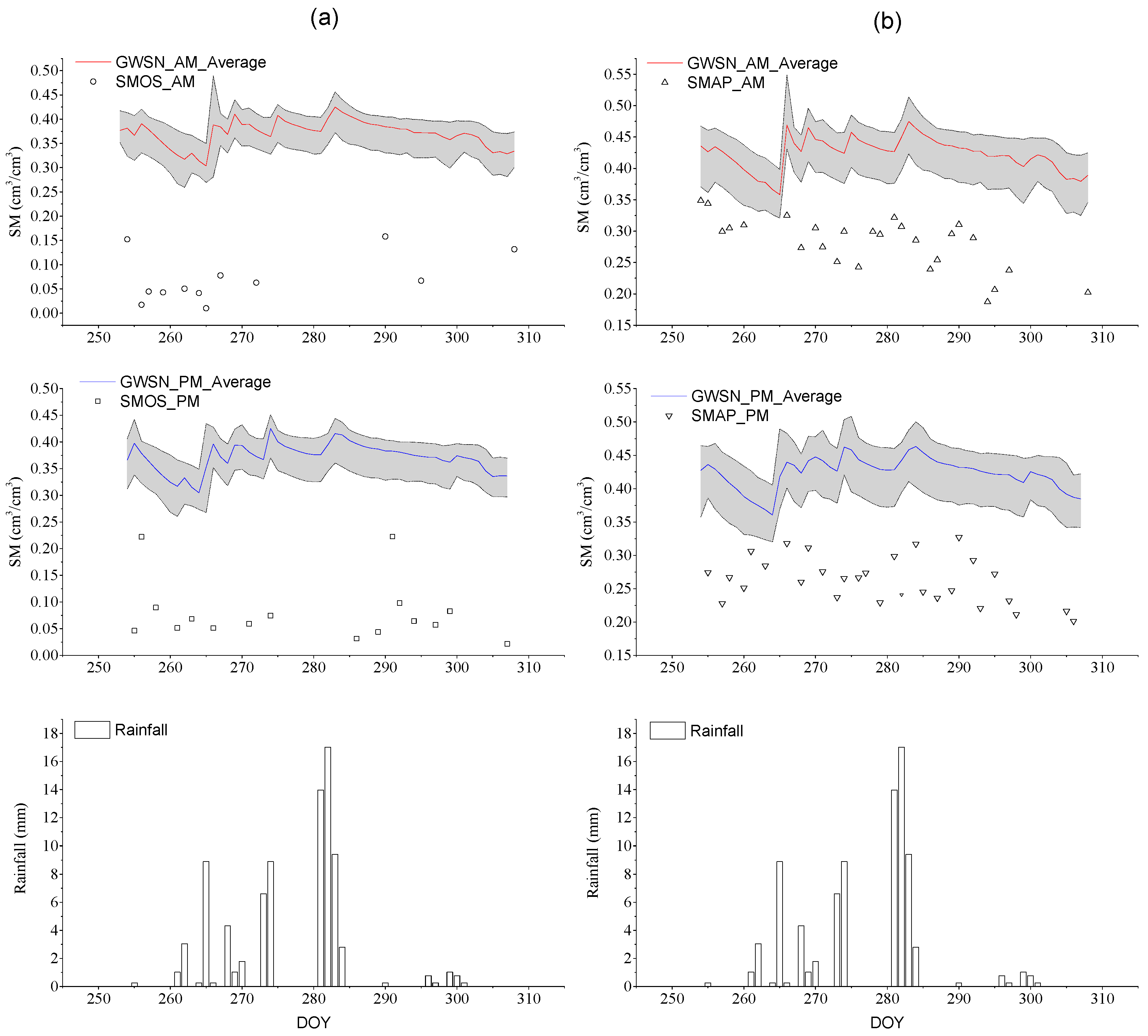
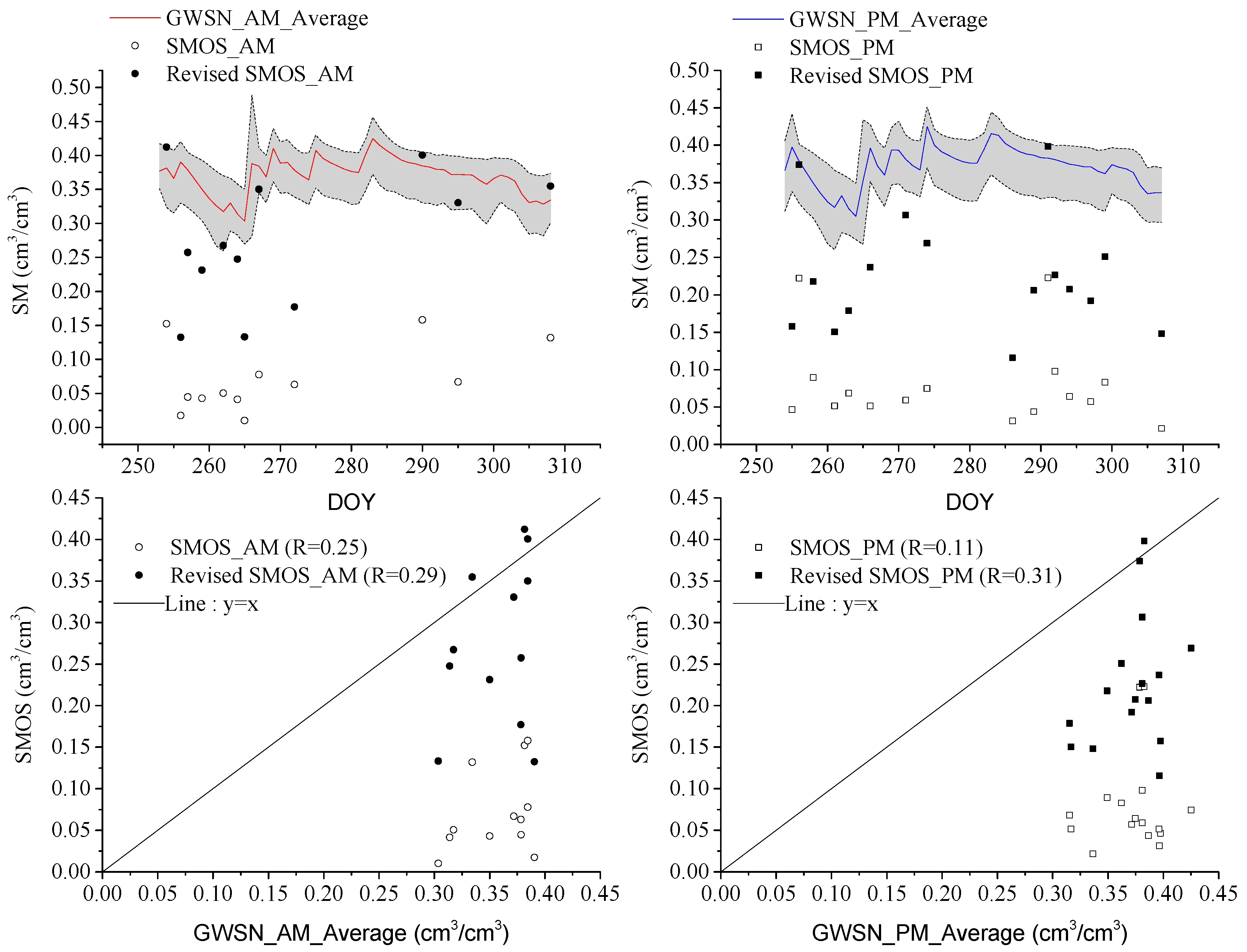
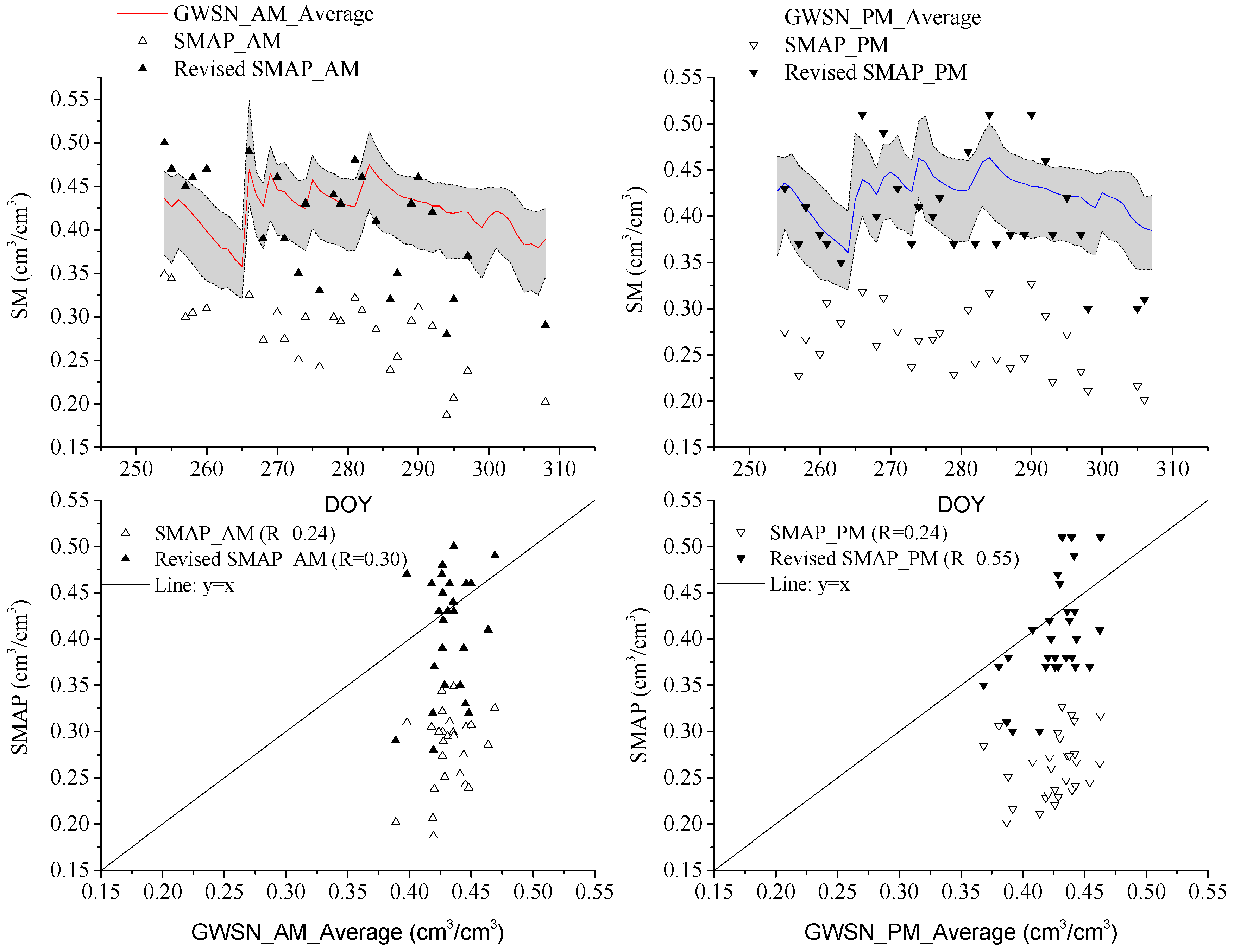
4.1. Comparison of SMOS/SMAP L3 Data with In-Situ Measurements
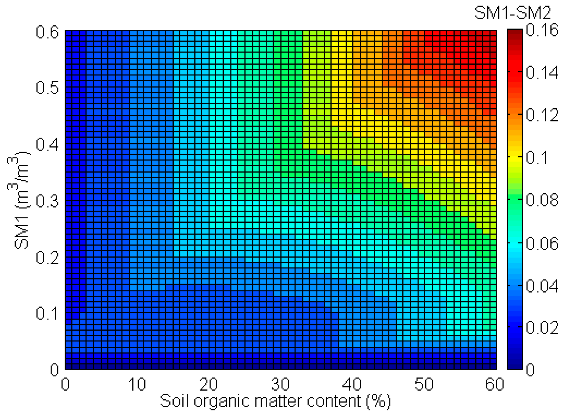
4.2. Liu’s Model Performance
4.3. Discussion
5. Conclusions
Acknowledgments
Author Contributions
Conflicts of Interest
References
- Kerr, Y.H.; Waldteufel, P.; Richaume, P.; Wigneron, J.P.; Ferrazzoli, P.; Mahmoodi, A.; Al Bitar, A.; Cabot, F.; Gruhier, C.; Juglea, S.E.; et al. The SMOS Soil Moisture Retrieval Algorithm. Geosci. Remote Sens. 2012, 50, 1384–1403. [Google Scholar] [CrossRef]
- Jackson, T.J.; Schmugge, T.J. Vegetation effects on the microwave emission of soils. Remote Sens. Environ. 1991, 36, 203–212. [Google Scholar] [CrossRef]
- Wagner, W.; Blöschl, G.; Pampaloni, P.; Calvet, J.-C.; Bizzarri, B.; Wigneron, J.-P.; Kerr, Y. Operational readiness of microwave remote sensing of soil moisture for hydrologic applications. Nord. Hydrol. 2007, 38, 1–20. [Google Scholar] [CrossRef]
- Ulaby, F.T.; Moore, R.K.; Fung, A.K. Microwave remote Sensing: Active and Passive. Volume 1—Microwave Remote Sensing Fundamentals and Radiometry; Addison-Wesley Publishing Company: New Jersey, NJ, USA, 1981. [Google Scholar]
- Ulaby, F.T.; Moore, R.K.; Fung, A.K. Microwave Remote Sensing: Active and Passive. Volume 2—Radar Remote Sensing and Surface Scattering and Emission Theory; Addison-Wesley Publishing Company: New Jersey, NJ, USA, 1982. [Google Scholar]
- Grant, J.P.; Wigneron, J.P.; Van De Griend, A.A.; Guglielmetti, M.; Saleh, K.; Schwank, M. Calibration of L-MEB for soil moisture retrieval over forests. In Proceedings of the IEEE International Geoscience & Remote Sensing Symposium, IGARSS 2007, Barcelona, Spain, 23–28 July 2007. [Google Scholar]
- Rahmoune, R.; Ferrazzoli, P.; Singh, Y.K.; Kerr, Y.H.; Richaume, P.; Al Bitar, A. SMOS retrieval results over forests: Comparisons with independent measurements. IEEE J. Sel. Top. Appl. Earth Obs. Remote Sens. 2014, 7, 3858–3866. [Google Scholar] [CrossRef]
- Rahmoune, R.; Ferrazzoli, P.; Kerr, Y.H.; Richaume, P. SMOS level 2 retrieval algorithm over forests: Description and generation of global maps. IEEE J. Sel. Top. Appl. Earth Obs. Remote Sens. 2013, 6, 1430–1439. [Google Scholar] [CrossRef]
- Wigneron, J.P.; Kerr, Y.; Waldteufel, P.; Saleh, K.; Escorihuela, M.J.; Richaume, P.; Ferrazzoli, P.; de Rosnay, P.; Gurney, R.; Calvet, J.C.; et al. L-band Microwave Emission of the Biosphere (L-MEB) Model: Description and calibration against experimental data sets over crop fields. Remote Sens. Environ. 2007, 107, 639–655. [Google Scholar] [CrossRef]
- Grant, J.P.; Saleh-Contell, K.; Wigneron, J.P.; Guglielmetti, M.; Kerr, Y.H.; Schwank, M.; Skou, N.; Van De Griend, A.A. Calibration of the L-MEB model over a coniferous and a deciduous forest. IEEE Trans. Geosci. Remote Sens. 2008, 46, 808–818. [Google Scholar] [CrossRef]
- Schwank, M.; Guglielmetti, M.; Mätzler, C.; Flühler, H. Testing a new model for the L-band radiation of moist leaf litter. IEEE Trans. Geosci. Remote Sens. 2008, 46, 1982–1994. [Google Scholar] [CrossRef]
- Kurum, M.; O’Neill, P.E.; Lang, R.H.; Cosh, M.H.; Joseph, A.T.; Jackson, T.J. Impact of conifer forest litter on microwave emission at L-band. IEEE Trans. Geosci. Remote Sens. 2012, 50, 1071–1084. [Google Scholar] [CrossRef]
- Della Vecchia, A.; Ferrazzoli, P.; Wigneron, J.P.; Grant, J.P. Modeling forest emissivity at L-band and a comparison with multitemporal measurements. IEEE Geosci. Remote Sens. Lett. 2007, 4, 508–512. [Google Scholar] [CrossRef]
- Lawrence, H.; Wigneron, J.P.; Demontoux, F.; Mialon, A.; Kerr, Y.H. Evaluating the semiempirical H-Q model used to calculate the l-band emissivity of a rough bare soil. IEEE Trans. Geosci. Remote Sens. 2013, 51, 4075–4084. [Google Scholar] [CrossRef]
- Parrens, M.; Wigneron, J.P.; Richaume, P.; Mialon, A.; Al Bitar, A.; Fernandez-Moran, R.; Al-Yaari, A.; Kerr, Y.H. Global-scale surface roughness effects at L-band as estimated from SMOS observations. Remote Sens. Environ. 2016, 181, 122–136. [Google Scholar] [CrossRef]
- Fernandez-Moran, R.; Wigneron, J.P.; Lopez-Baeza, E.; Al-Yaari, A.; Coll-Pajaron, A.; Mialon, A.; Miernecki, M.; Parrens, M.; Salgado-Hernanz, P.M.; Schwank, M.; et al. Roughness and vegetation parameterizations at L-band for soil moisture retrievals over a vineyard field. Remote Sens. Environ. 2015, 170, 269–279. [Google Scholar] [CrossRef]
- Wigneron, J.-P.; Laguerre, L.; Kerr, Y.H. A simple parameterization of the L-band microwave emission from rough agricultural soils. IEEE Trans. Geosci. Remote Sens. 2001, 39, 1697–1707. [Google Scholar] [CrossRef]
- O’Neill, P.; Chan, S.; Njoku, E.; Jackson, T.; Bindlish, R. Soil Moisture Active Passive (SMAP): Algorithm Theoretical Basis Document, SMAP L2 & L3 Soil Moisture (Passive) Data Products; Jet Propulsion Laboratory: Pasadena, CA, USA, 2015. [Google Scholar]
- Array Systems Computing Inc. Algorithm Theoretical Basis Document (ATBD) for the SMOS Level 2 Soil Moisture Processor Development Continuation Project; Array Systems Computing Inc.: North York, ON, Canada, 2014; pp. 26–59. [Google Scholar]
- Wang, J.R. The dielectric properties of soil-water mixtures at microwave frequencies. Radio Sci. 1980, 15, 977–985. [Google Scholar] [CrossRef]
- Dobson, M.C.; Ulaby, F.T.; Hallikainen, M.T.; El-Rayes, M.A. Microwave Dielectric Behavior of Wet Soil-Part II: Dielectric Mixing Models. IEEE Trans. Geosci. Remote Sens. 1985, GE-23, 35–46. [Google Scholar] [CrossRef]
- Mironov, V.L.; Kosolapova, L.G.; Fomin, S.V. Physically and mineralogically based spectroscopic dielectric model for moist soils. IEEE Trans. Geosci. Remote Sens. 2009, 47, 2059–2070. [Google Scholar] [CrossRef]
- Malicki, M.A.; Plagge, R.; Roth, C.H. Improving the calibration of dielectric TDR soil moisture determination taking into account the solid soil. Eur. J. Soil Sci. 1996, 47, 357–366. [Google Scholar] [CrossRef]
- De Jong, R.; Campbell, C.A.; Nicholaichuk, W. Water retention equations and their relationship to soil organic matter and particle size distribution for disturbed samples. Can. J. Soil Sci. 1983, 63, 291–302. [Google Scholar] [CrossRef]
- Jones, S.B.; Wraith, J.M.; Or, D. Time domain reflectometry measurement principles and applications. Hydrol. Process. 2002, 16, 141–153. [Google Scholar] [CrossRef]
- Bircher, S.; Demontoux, F.; Razafindratsima, S.; Zakharova, E.; Drusch, M.; Wigneron, J.-P.; Kerr, Y. L-Band Relative Permittivity of Organic Soil Surface Layers—A New Dataset of Resonant Cavity Measurements and Model Evaluation. Remote Sens. 2016, 8, 1024. [Google Scholar] [CrossRef]
- Mironov, V.L.; Bobrov, P.P. Soil dielectric spectroscopic parameters dependence on humus content. In Proceedings of the 2003 IEEE International Geoscience and Remote Sensing Symposium, Toulouse, France, 21–25 July 2003; pp. 1106–1108. [Google Scholar]
- Mironov, V.; Savin, I. A temperature-dependent multi-relaxation spectroscopic dielectric model for thawed and frozen organic soil at 0.05–15 GHz. Phys. Chem. Earth 2015, 83–84, 57–64. [Google Scholar] [CrossRef]
- Liu, J.; Zhao, S.; Jiang, L.; Chai, L.; Wu, F. The influence of organic matter on soil dielectric constant at microwave frequencies (0.5–40 GHZ). In Proceedings of the 2013 IEEE International Geoscience and Remote Sensing Symposium, Melbourne, Australia, 21–26 July 2013; pp. 13–16. [Google Scholar]
- FAO/IIASA/ISRIC/ISSCAS/JRC. Harmonized World Soil Database (Version 1.2); FAO: Rome, Italy; IIASA: Laxenburg, Austria, 2012. [Google Scholar]
- Cosh, M.H.; Jackson, T.J.; Bindlish, R.; Prueger, J.H. Watershed scale temporal and spatial stability of soil moisture and its role in validating satellite estimates. Remote Sens. Environ. 2004, 92, 427–435. [Google Scholar] [CrossRef]
- EC-5 Soil Moisture Sensor; Operator’s Manual; Decagon Devices, Inc.: Pullman, USA, 2016; Available online: http://www.decagon.com/en/soils/volumetric-water-content-sensors/ec-5-lowest-cost-vwc/ (accessed on 10 October 2016).
- Bircher, S.; Andreasen, M.; Vuollet, J.; Vehviläinen, J.; Rautiainen, K.; Jonard, F.; Weihermüller, L.; Zakharova, E.; Wigneron, J.P.; Kerr, Y.H. Soil moisture sensor calibration for organic soil surface layers. Geosci. Instrum. Methods Data Syst. 2016, 5, 109–125. [Google Scholar] [CrossRef]
- Brodzik, M.J.; Billingsley, B.; Haran, T.; Raup, B.; Savoie, M.H. EASE-Grid 2.0: Incremental but Significant Improvements for Earth-Gridded Data Sets. ISPRS Int. J. Geo-Inf. 1990, 1, 32–45. [Google Scholar] [CrossRef]
- Kerr, Y.H.; Jacquette, E.; Al Bitar, A.; Cabot, F.; Mialon, A.; Richaume, P. CATDS SMOS L3 Soil Moisture Retrieval Processor; Algorithm Theoretical Baseline Document (ATBD); CESBIO: Toulouse, France, 2013; p. 73. [Google Scholar]
- Entekhabi, D.; Reichle, R.H.; Koster, R.D.; Crow, W.T. Performance Metrics for Soil Moisture Retrievals and Application Requirements. J. Hydrometeorol. 2010, 11, 832–840. [Google Scholar] [CrossRef]
- Wang, J.R.; O’Neill, P.E.; Jackson, T.J.; Engman, E.T. Multifrequency Measurements of the Effects of Soil Moisture, Soil Texture, and Surface Roughness. IEEE Trans. Geosci. Remote Sens. 1983, GE-21, 44–51. [Google Scholar] [CrossRef]
- Montpetit, B.; Royer, A.; Wigneron, J.P.; Chanzy, A.; Mialon, A. Evaluation of multi-frequency bare soil microwave reflectivity models. Remote Sens. Environ. 2015, 162, 186–195. [Google Scholar] [CrossRef]
- Saleh, K.; Wigneron, J.P.; De Rosnay, P.; Calvet, J.C.; Escorihuela, M.J.; Kerr, Y.; Waldteufel, P. Impact of rain interception by vegetation and mulch on the L-band emission of natural grass. Remote Sens. Environ. 2006, 101, 127–139. [Google Scholar] [CrossRef]
- Jackson, T.J.; Bindlish, R.; Cosh, M.H.; Zhao, T.; Starks, P.J.; Bosch, D.D.; Seyfried, M.; Moran, M.S.; Goodrich, D.C.; Kerr, Y.H.; et al. Validation of soil moisture and Ocean Salinity (SMOS) soil moisture over watershed networks in the U.S. IEEE Trans. Geosci. Remote Sens. 2012, 50, 1530–1543. [Google Scholar] [CrossRef]
- Grant, J.P.; van de Griend, A.A.; Schwank, M.; Wigneron, J.P. Observations and modeling of a pine forest floor at L-band. IEEE Trans. Geosci. Remote Sens. 2009, 47, 2024–2034. [Google Scholar] [CrossRef]
- Grant, J.P.; Wigneron, J.P.; Van de Griend, A.A.; Kruszewski, A.; Søbjærg, S.S.; Skou, N. A field experiment on microwave forest radiometry: L-band signal behaviour for varying conditions of surface wetness. Remote Sens. Environ. 2007, 109, 10–19. [Google Scholar] [CrossRef]
- Putuhena, W.M.; Cordery, I. Estimation of interception capacity of the forest floor. J. Hydrol. 1996, 180, 283–299. [Google Scholar] [CrossRef]
- Wigneron, J.-P.; Calvet, J.-C.; Kerr, Y. Monitoring water interception by crop fields from passive microwave observations. Agric. For. Meteorol. 1996, 80, 177–194. [Google Scholar] [CrossRef]
- Burke, E.J.; Wigneron, J.P.; Gurney, R.J. The comparison of two models that determine the effects of a vegetation canopy on passive microwave emission. Hydrol. Earth Syst. Sci. 1999, 3, 439–444. [Google Scholar] [CrossRef]
- Utku, C.; Le Vine, D.M. A model for prediction of the impact of topography on microwave emission. IEEE Trans. Geosci. Remote Sens. 2011, 49, 395–405. [Google Scholar] [CrossRef]


| Site | Soil Type | SN | Clay | Silt | Sand |
|---|---|---|---|---|---|
| 1 | Silt Loam | 25 | 14.21 | 66.48 | 19.31 |
| 2 | Silt Loam | 25 | 12.90 | 60.28 | 26.82 |
| 3 | Silt Loam | 25 | 12.37 | 67.66 | 19.97 |
| 4 | Silt Loam | 25 | 13.59 | 62.60 | 23.81 |
| 5 | Silt Loam | 20 | 12.32 | 69.01 | 18.67 |
| 6 | Silt Loam | 25 | 10.81 | 67.12 | 22.07 |
| Statistical Indicators | Satellite SM Retrievals with Mironov Model | Revised SM Retrievals with Liu’s Model | ||||||
|---|---|---|---|---|---|---|---|---|
| SMOS AM | SMOS PM | SMAP AM | SMAP PM | SMOS AM | SMOS PM | SMAP AM | SMAP PM | |
| Bias | 0.29 | 0.29 | 0.15 | 0.16 | 0.08 | 0.14 | 0.02 | 0.02 |
| RMSE | 0.30 | 0.31 | 0.16 | 0.17 | 0.13 | 0.17 | 0.07 | 0.05 |
| ubRMSE | 0.10 | 0.10 | 0.05 | 0.05 | 0.10 | 0.08 | 0.06 | 0.05 |
| R | 0.25 | 0.11 | 0.24 | 0.24 | 0.29 | 0.31 | 0.24 | 0.55 |
© 2017 by the authors. Licensee MDPI, Basel, Switzerland. This article is an open access article distributed under the terms and conditions of the Creative Commons Attribution (CC BY) license (http://creativecommons.org/licenses/by/4.0/).
Share and Cite
Jin, M.; Zheng, X.; Jiang, T.; Li, X.; Li, X.-J.; Zhao, K. Evaluation and Improvement of SMOS and SMAP Soil Moisture Products for Soils with High Organic Matter over a Forested Area in Northeast China. Remote Sens. 2017, 9, 387. https://0-doi-org.brum.beds.ac.uk/10.3390/rs9040387
Jin M, Zheng X, Jiang T, Li X, Li X-J, Zhao K. Evaluation and Improvement of SMOS and SMAP Soil Moisture Products for Soils with High Organic Matter over a Forested Area in Northeast China. Remote Sensing. 2017; 9(4):387. https://0-doi-org.brum.beds.ac.uk/10.3390/rs9040387
Chicago/Turabian StyleJin, Mengjie, Xingming Zheng, Tao Jiang, Xiaofeng Li, Xiao-Jie Li, and Kai Zhao. 2017. "Evaluation and Improvement of SMOS and SMAP Soil Moisture Products for Soils with High Organic Matter over a Forested Area in Northeast China" Remote Sensing 9, no. 4: 387. https://0-doi-org.brum.beds.ac.uk/10.3390/rs9040387