
Compact Polarimetric Response of Rape (Brassica napus L.) at C-Band: Analysis and Growth Parameters Inversion

 ,
, 
Abstract
:
1. Introduction
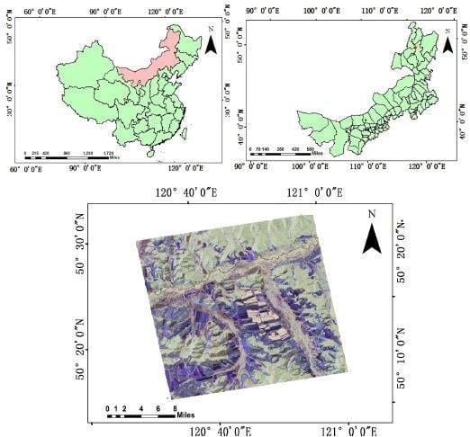
2. Test Sites, SAR Data and Ground Measurement Campaign
3. FP SAR Data Processing and Compact Polarimetric SAR Data Simulation
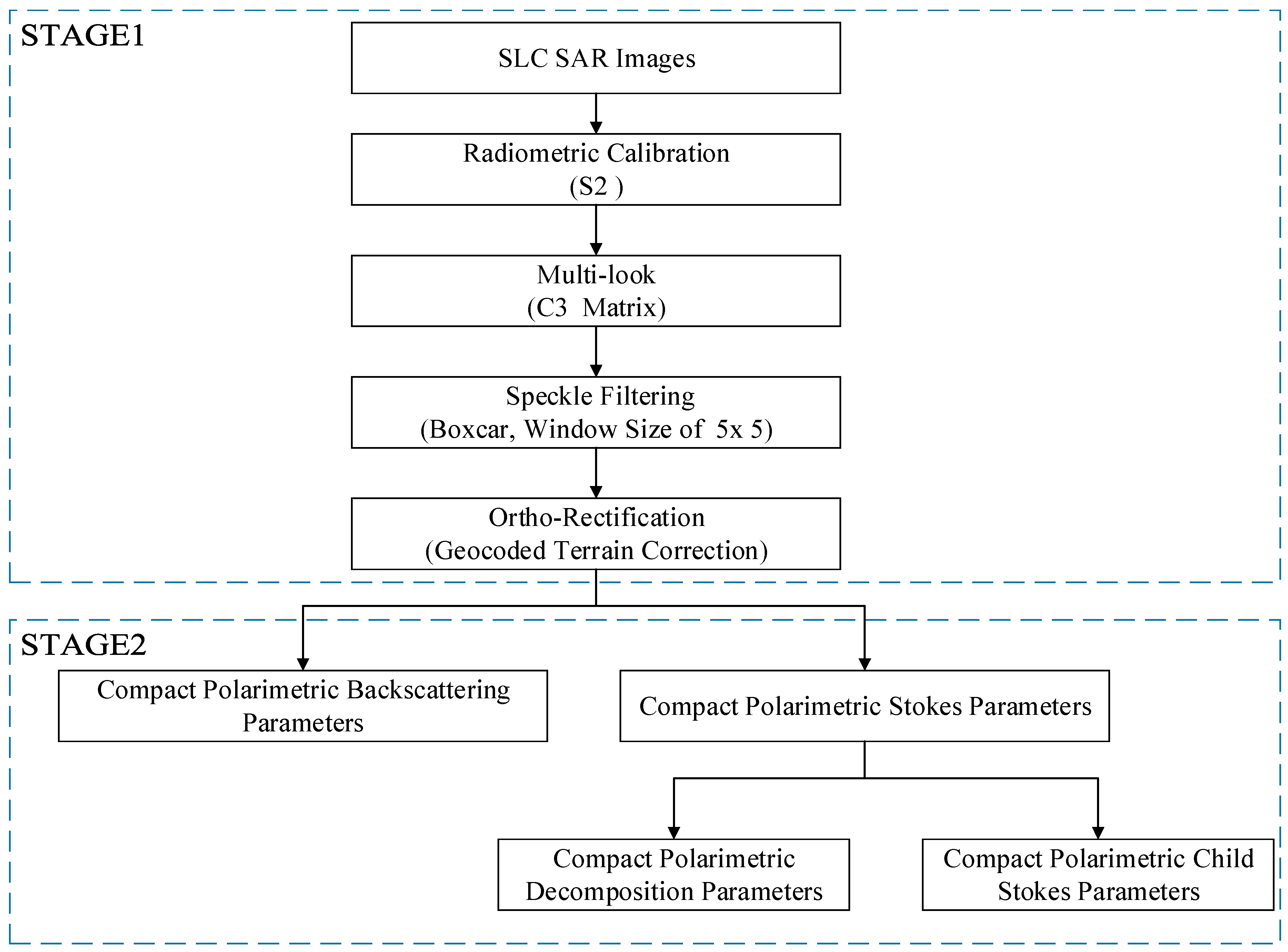
3.1. FP SAR Data Processing
3.2. Compact Polarimetric SAR Data Simulation
4. Approach and Methods
4.1. Extraction of Compact Polarimetric Parameters
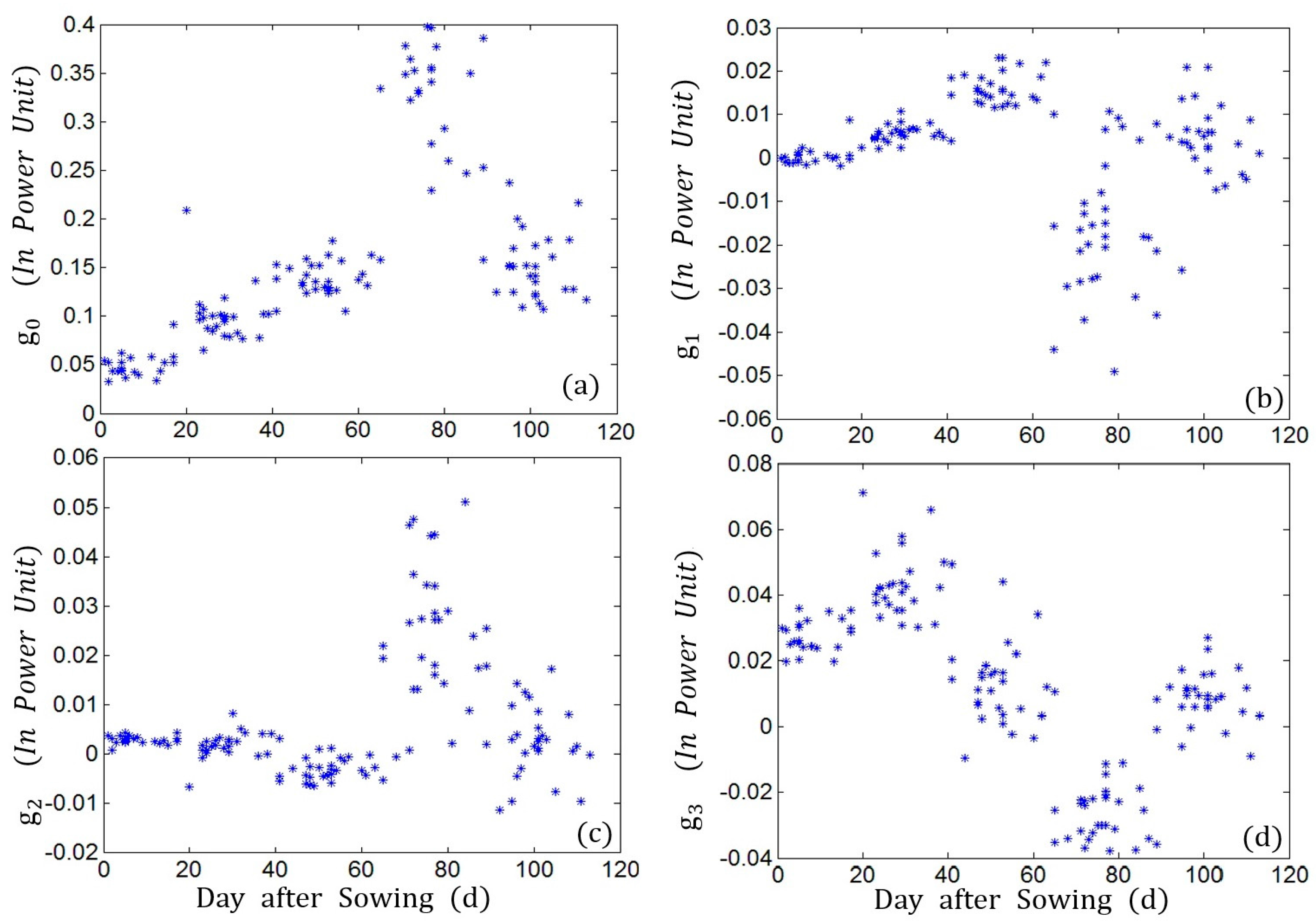
4.1.1. Stokes Parameters
4.1.2. Stokes Child Parameters
4.1.3. Backscattering Parameters
4.1.4. Decomposition Parameters
4.2. Random Forest Regression Algorithm for Rape Growth Parameters Inversion
5. Results
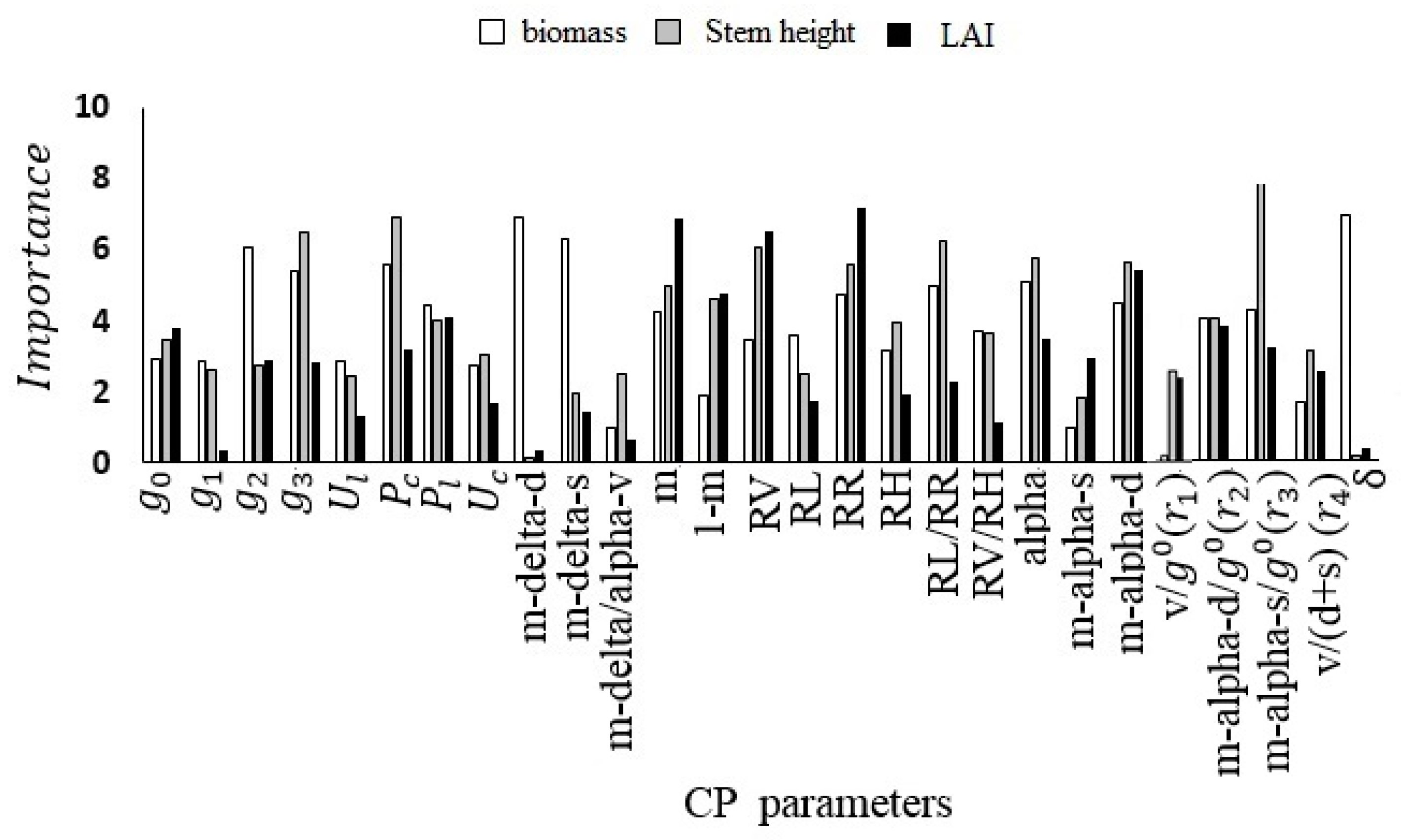
5.1. Analysis of CP Observables’ Sensitivity to Rape Growth Parameters
5.1.1. Stokes Parameters
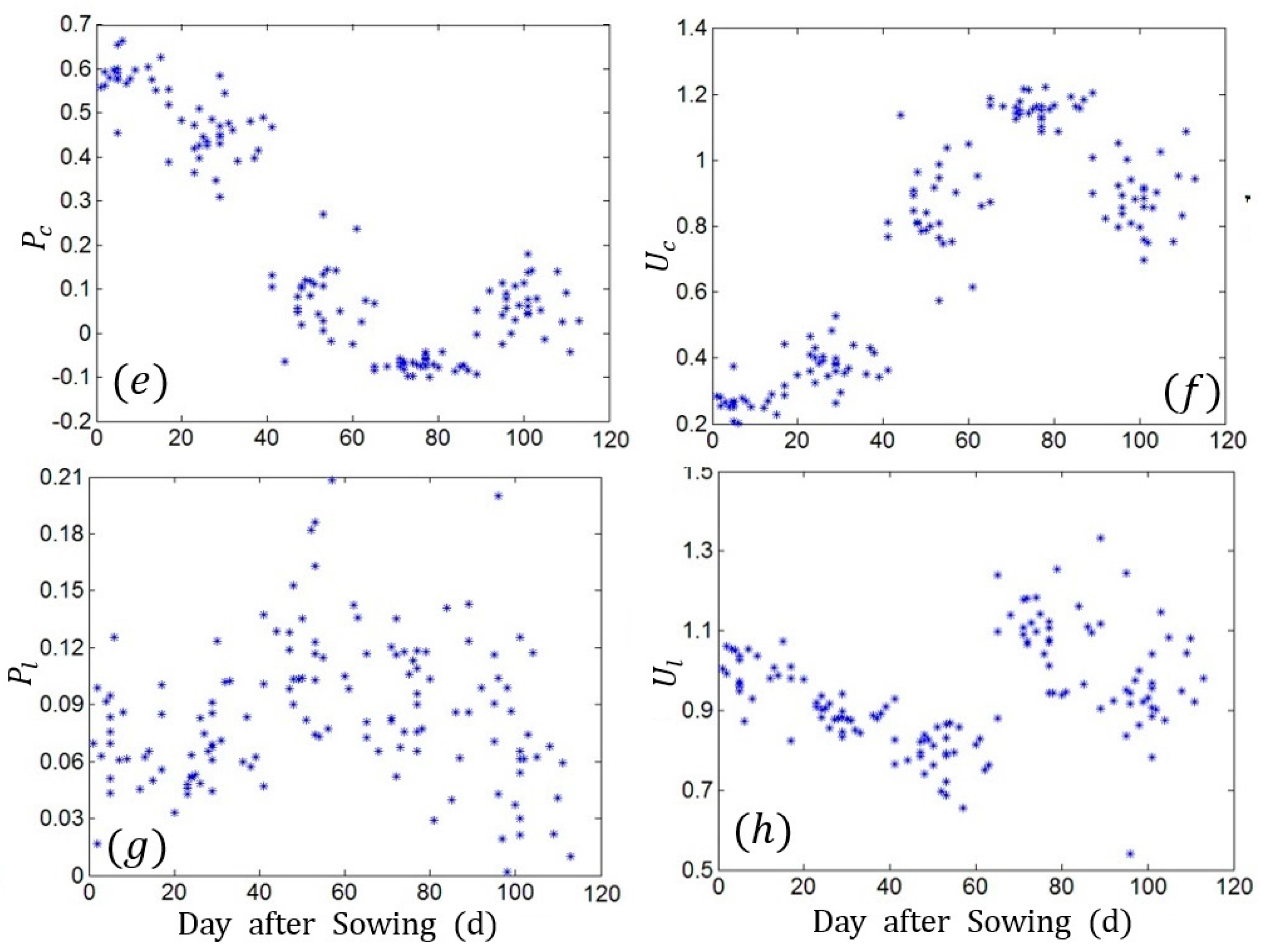
5.1.2. Stokes Child Parameters
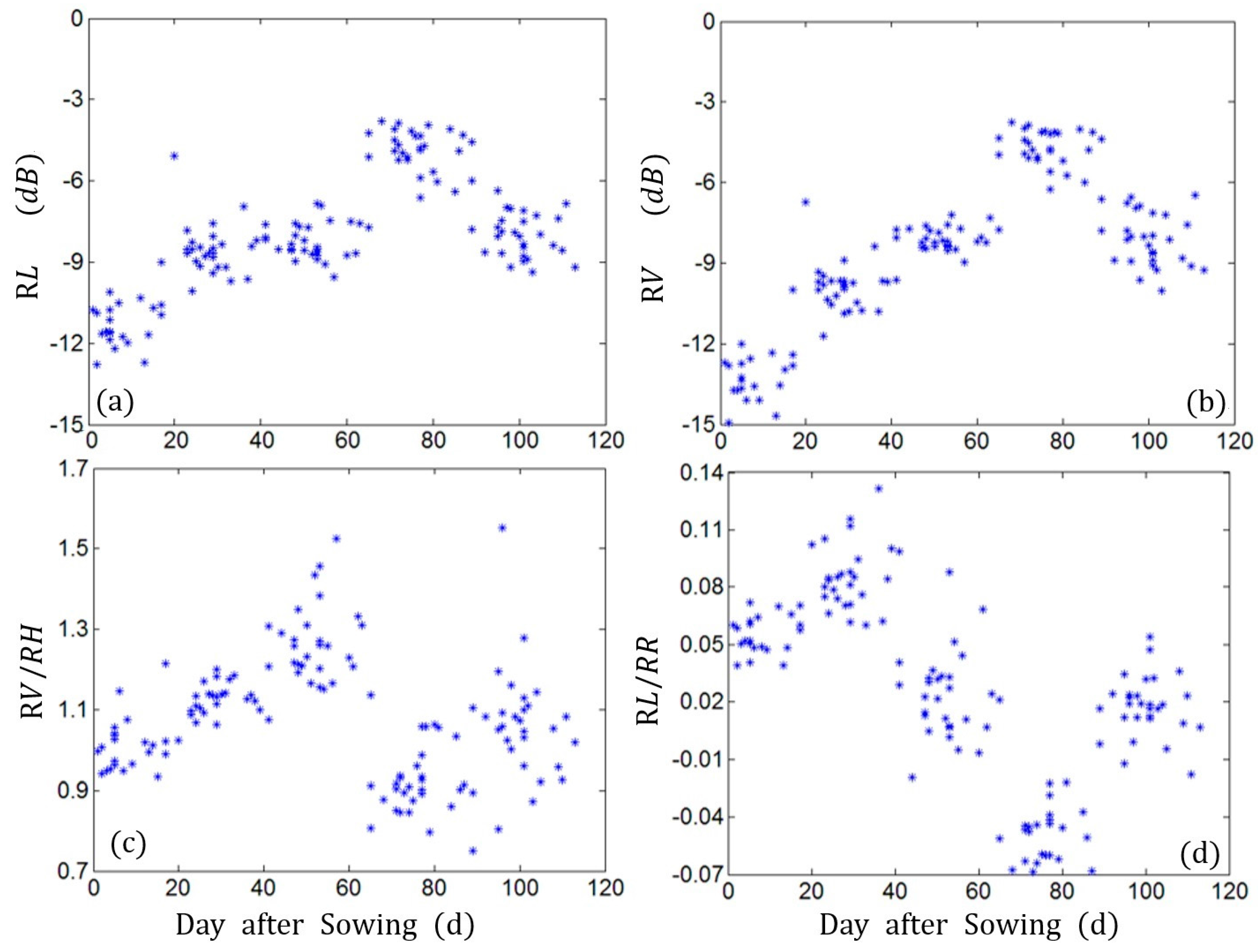
5.1.3. Backscattering Parameters
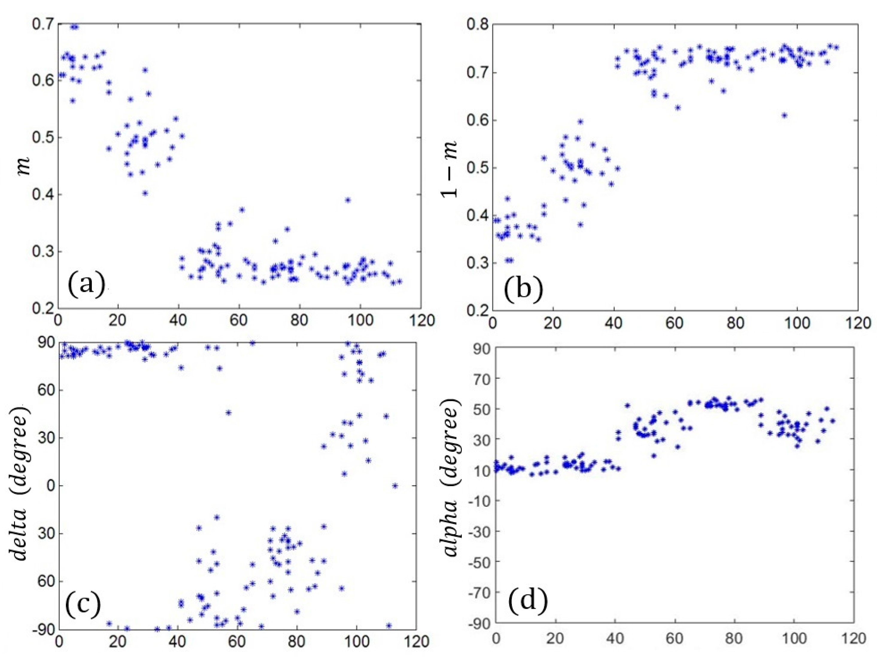
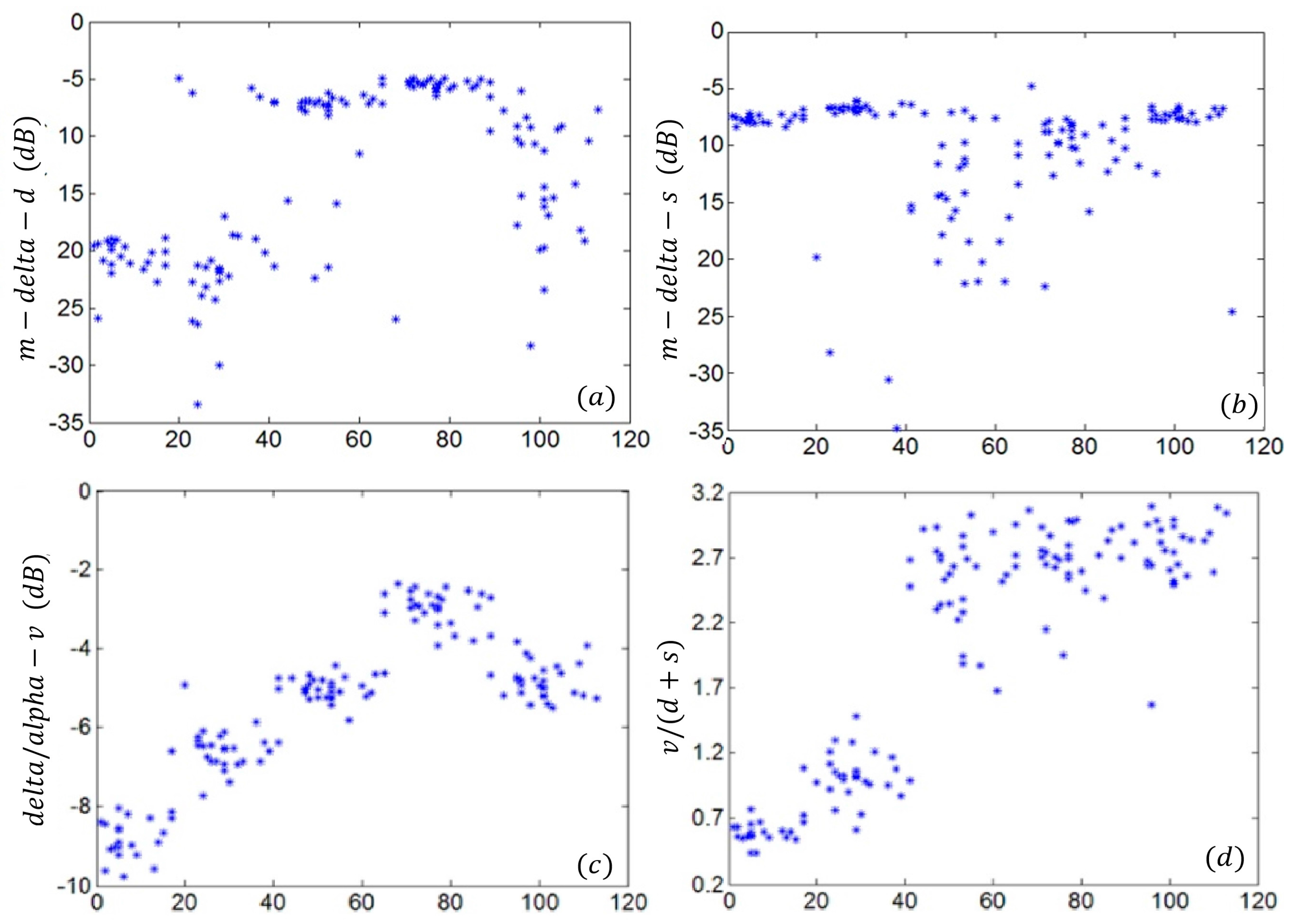
5.1.4. Decomposition Parameters
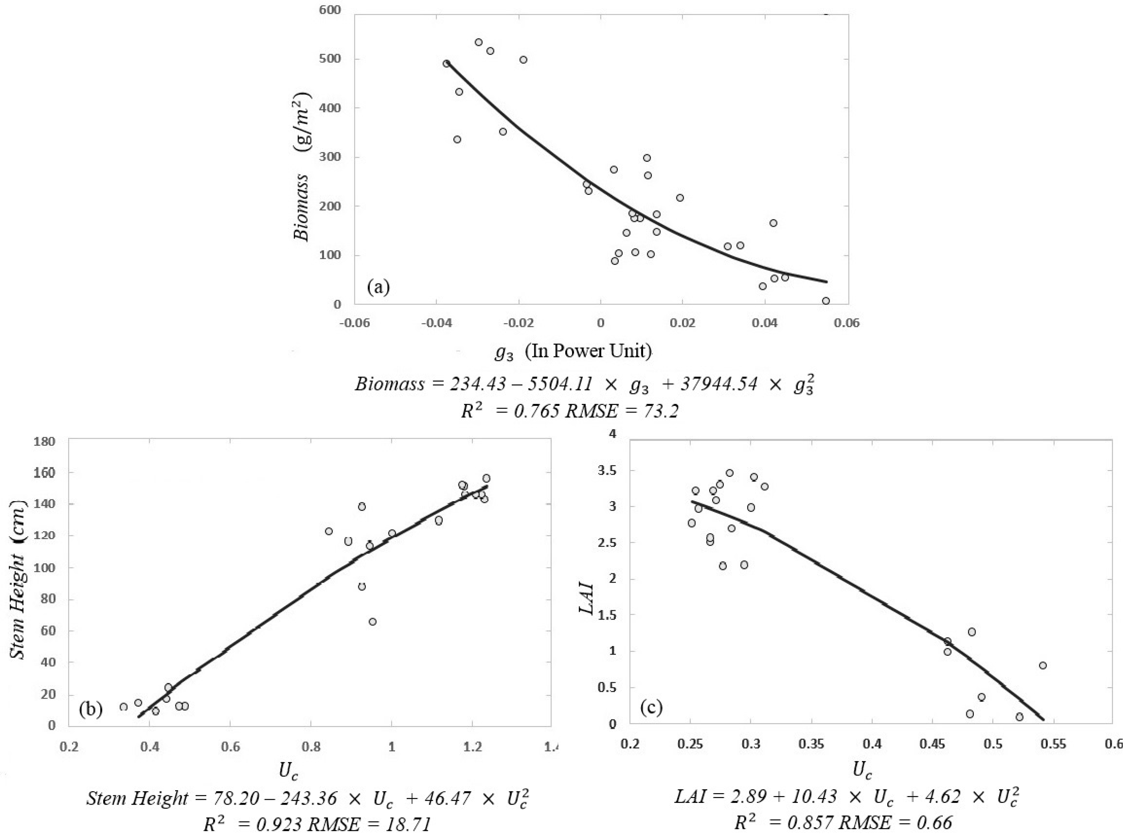
5.2. Growth Parameters Inversion with Random Forest
6. Discussion
7. Conclusions
Acknowledgments
Author Contributions
Conflicts of Interest
References
- Liu, C. Development of Rapeseed Production and Bio-Diesel in China; Huazhong Agricultural University: Wuhan, China, 2008. [Google Scholar]
- Liu, J.; Pattey, E.; Jégo, G. Assessment of vegetation indices for regional crop green LAI estimation from Landsat images over multiple growing seasons. Remote Sens. Environ. 2012, 123, 347–358. [Google Scholar] [CrossRef]
- Lopez-Sanchez, J.M.; Vicente-Guijalba, F.; Ballester-Berman, J.D.; Cloude, S.R. Polarimetric Response of Rice Fields at C-Band: Analysis and Phenology Retrieval. IEEE Trans. Geosci. Remote Sens. 2014, 52, 2977–2993. [Google Scholar] [CrossRef]
- Wang, L.A.; Zhou, W.; Zhu, X.K.; Dong, Z.D.; Guo, W.S. Estimation of biomass in wheat using random forest regression algorithm and remote sensing data. Crop J. 2016, 4, 212–219. [Google Scholar] [CrossRef]
- Jia, Y.Z.; Li, B.; Cheng, Y.Z.; Liu, T.; Guo, Y.; Wu, X.H.; Wang, L.G. Comparison between GF-1 images and Landsat-8 images in monitoring maize LAI. Trans. Chin. Soc. Agric. Eng. 2015, 31, 173–179. [Google Scholar]
- Skriver, H. Crop Classification by Multitemporal C- and L-Band Single- and Dual-Polarization and Fully Polarimetric SAR. IEEE Trans. Geosci. Remote Sens. 2012, 50, 2138–2149. [Google Scholar] [CrossRef]
- Küçük, Ç.; Taşkın, G.; Erten, E. Paddy-Rice Phenology Classification Based on Machine-Learning Methods Using Multitemporal Co-Polar X-Band SAR Images. IEEE. Sel. Top. Appl. Earth Obs. Remote Sens. 2016, 9, 2509–2519. [Google Scholar] [CrossRef]
- Hoang, H.K.; Bernier, M.; Duchesne, S.; Tran, Y.M. Rice Mapping Using RADARSAT-2 Dual- and Quad-Pol Data in a Complex Land-Use Watershed: Cau River Basin (Vietnam). IEEE J. Sel. Top. Appl. Earth Obs. Remote Sens. 2016, 9, 3082–3096. [Google Scholar] [CrossRef]
- Lopez-Sanchez, J.M.; Cloude, S.R.; Ballester-Berman, J.D. Rice Phenology Monitoring by Means of SAR Polarimetry at X-Band. IEEE Trans. Geosci. Remote Sens. 2012, 50, 2695–2709. [Google Scholar] [CrossRef]
- Jin, X.; Yang, G.; Xu, X.; Yang, H.; Feng, H. Combined Multi-Temporal Optical and Radar Parameters for Estimating LAI and Biomass in Winter Wheat Using HJ and RADARSAR-2 Data. Remote Sens. 2015, 7, 13251–13272. [Google Scholar] [CrossRef]
- Jia, M.; Tong, W.; Zhang, Y.; Chen, Y. Rice Biomass Estimation Using Radar Backscattering Data at S-band. IEEE J. Sel. Top. Appl. Earth Obs. Remote Sens. 2014, 7, 469–479. [Google Scholar] [CrossRef]
- Alberti, G.; Candido, P.; Peressotti, A.; Turco, S.; Piussi, P.; Zerbi, G. Abstract and Résumé. Aboveground biomass relationships for mixed ash (L. and Hudson) stands in Eastern Prealps of Friuli Venezia Giulia (Italy). Ann. For. Sci. 2005, 62, 831–836. [Google Scholar] [CrossRef]
- Cloude, S. Polarisation: Applications in Remote Sensing, 1st ed.; Oxford University Press: Oxford, UK, 2009. [Google Scholar]
- Rui, Y.K.; Peng, Y.F.; Wang, Z.R.; Shen, J.B. Stem perimeter, height and biomass of maize (Zea mays L.) grown under different N fertilization regimes in Beijing, China. Int. J. Plant Prod. 2009, 3, 85–90. [Google Scholar]
- Shang, F.; Hirose, A. Averaged Stokes Vector Based Polarimetric SAR Data Interpretation. IEEE Trans. Geosci. Remote Sens. 2015, 53, 4536–4547. [Google Scholar] [CrossRef]
- Cloude, S.R.; Pottier, E. A review of target decomposition theorems in radar polarimetry. IEEE Trans. Geosci. Remote Sens. 1996, 34, 498–518. [Google Scholar] [CrossRef]
- Raney, R.K. Hybrid-Polarity SAR Architecture. IEEE Trans. Geosci. Remote Sens. 2007, 45, 3397–3404. [Google Scholar] [CrossRef]
- Raney, R.K. Dual-polarized SAR and Stokes parameters. IEEE Geosci. Remote Sens. Lett. 2006, 3, 317–319. [Google Scholar] [CrossRef]
- Steele-Dunne, S.C.; McNairn, H.; Monsivais-Huertero, A. Radar Remote Sensing of Agricultural Canopies: A Review. IEEE J. Sel. Top. Appl. Earth Obs. Remote Sens. 2017, 10, 2249–2273. [Google Scholar] [CrossRef]
- Mcnairn, H.; Shang, J.; Champagne, C.; Jiao, X. TerraSAR-X and RADARSAT-2 for crop classification and acreage estimation. In Proceedings of the 2009 IEEE International Geoscience and Remote Sensing Symposium, Cape Town, South Africa, 12–17 July 2009. [Google Scholar]
- Charbonneau, F.J.; Brisco, B.; Raney, R.K.; McNairn, H.; Liu, C.; Vachon, P.W.; Shang, J.; DeAbreu, R.; Chanmpagne, C.; Merzouki, A.; et al. Compact polarimetry overview and applications assessment. Can. J. Remote Sens. 2014, 36, 298. [Google Scholar] [CrossRef]
- Nord, M.E.; Ainsworth, T.L.; Lee, J.S.; Stacy, N.J.S. Comparison of Compact Polarimetric Synthetic Aperture Radar Modes. IEEE Trans. Geosci. Remote Sens. 2009, 47, 174–188. [Google Scholar] [CrossRef]
- Yang, Z.; Li, K.; Liu, L.; Shao, Y.; Brisco, B.; Li, W.G. Rice growth monitoring using simulated compact polarimetric C band SAR. Radio Sci. 2014, 49, 1300–1315. [Google Scholar] [CrossRef]
- Cloude, S.R.; Goodenough, D.G.; Chen, H. Compact Decomposition Theory. Geosci. Remote Sens. Lett. IEEE 2012, 9, 28–32. [Google Scholar] [CrossRef]
- Yang, H.; Xie, L.; Chen, E.X.; Zhang, H.; Yang, G.J.; Li, Z.H.; Gu, X.H. Biomass estimation of oilseed rape using simulated compact polarimtric SAR imagery. In Proceedings of the 2016 IEEE International Geoscience and Remote Sensing Symposium (IGARSS), Beijing, China, 10–15 July 2016. [Google Scholar]
- Tottman, D.R. The decimal code for the growth stages of cereals, with illustrations. Ann. Appl. Biol. 2008, 110, 441–454. [Google Scholar] [CrossRef]
- Yang, H.; Li, Z.Y.; Chen, E.X.; Zhao, C.J.; Yang, G.J.; Casa, R.; Pignatti, S.; Feng, Q. Temporal Polarimetric Behavior of Oilseed Rape (Brassica napus L.) at C-Band for Early Season Sowing Date Monitoring. Remote Sens. 2014, 6, 10375–10394. [Google Scholar] [CrossRef]
- Raney, R.K.; Cahill, J.S.T.S.; Patterson, G.W.; Bussey, D.B.J. The m-chi decomposition of hybrid dual-polarimetric radar data. In Proceedings of the 2012 IEEE International Geoscience and Remote Sensing Symposium, Munich, Germany, 22–27 July 2012. [Google Scholar]
- Stokes, G.G. On the Composition and Resolution of Streams of Polarized Light from different Sources. Trans. Camb. Philos. Soc. 1851, 9, 399. [Google Scholar]
- Zhang, H.; Xie, L.; Wang, C.; Wu, F.; Zhang, B. Investigation of the Capability of H-α Decomposition of Compact Polarimetric SAR. IEEE Geosci. Remote Sens. Lett. 2014, 11, 868–872. [Google Scholar] [CrossRef]
- Breiman, L. Random Forests. Mach. Learn. 2001, 45, 5–32. [Google Scholar] [CrossRef]
- Cutler, A.; Cutler, D.R.; Stevens, J.R. Random Forests. Mach. Learn. 2012, 45, 157–176. [Google Scholar]
- Bouvet, A.; Toan, T.L.; Lam-Dao, N. Monitoring of the Rice Cropping System in the Mekong Delta Using ENVISAT/ASAR Dual Polarization Data. IEEE Trans. Geosci. Remote Sens. 2009, 47, 517–526. [Google Scholar] [CrossRef]
- Larranaga, A.; Alvarez-Mozos, J.; Albizua, L.; Peters, J. Backscattering Behavior of Rain-Fed Crops Along the Growing Season. Geosci. Remote Sens. Lett. IEEE 2013, 10, 386–390. [Google Scholar] [CrossRef]
- Born, M.; Wolf, E. Principles of Optics, 6th ed.; Cambridge University Press: Cambridge, UK, 1999. [Google Scholar]


| Parameters | Values |
|---|---|
| Polarization | Quad |
| Frequency | 5.405 GHz |
| Incidence angle | 37.4–38.8 |
| Range pixel spacing | 4.96 m |
| Azimuth pixel spacing | 4.73 m |
| Orbit direction | Ascending |
| Beam mode | FQ18 |
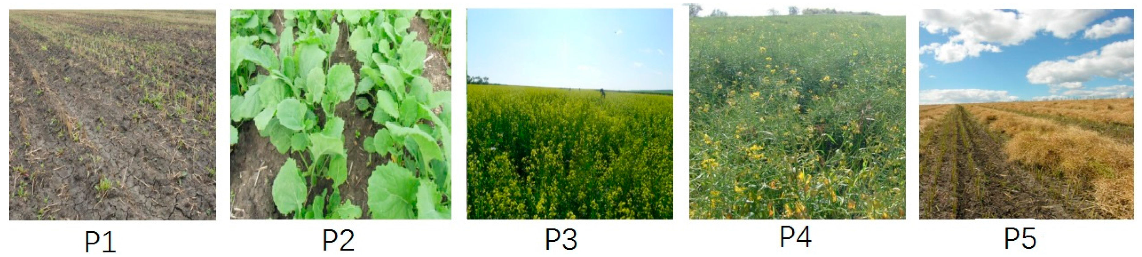
| Acquisition Date | BBCH Stages | Principal Scales (DAS) |
|---|---|---|
| 23 May 2013 | Germination (0) | P1 [–7, 15] |
| 16 June 2013 | Leaf development (1) and formation of side shoots (2) | P2 [16, 39] |
| 10 July 2013 | Stem elongation (3),inflorescence emergence (5) and flowering (6) | P3 [40, 63] |
| 3 August 2013 | Development of fruit (7) | P4 [64, 87] |
| 27 August 2013 | Ripening (8) and senescence (9) | P5 [89, 110] |
| Growth Parameters | RF-R2 | RF-RMSE | R2 (Regression Model) | RMSE (Regression Model) |
|---|---|---|---|---|
| Biomass | 0.93 | 46.24 g/m2 | 0.765 | 73.20 g/m2 |
| Stem height | 0.95 | 13.5 cm | 0.923 | 18.71 cm |
| LAI | 0.96 | 0.25 | 0.857 | 0.66 |
© 2017 by the authors. Licensee MDPI, Basel, Switzerland. This article is an open access article distributed under the terms and conditions of the Creative Commons Attribution (CC BY) license (http://creativecommons.org/licenses/by/4.0/).
Share and Cite
Zhang, W.; Li, Z.; Chen, E.; Zhang, Y.; Yang, H.; Zhao, L.; Ji, Y. Compact Polarimetric Response of Rape (Brassica napus L.) at C-Band: Analysis and Growth Parameters Inversion. Remote Sens. 2017, 9, 591. https://0-doi-org.brum.beds.ac.uk/10.3390/rs9060591
Zhang W, Li Z, Chen E, Zhang Y, Yang H, Zhao L, Ji Y. Compact Polarimetric Response of Rape (Brassica napus L.) at C-Band: Analysis and Growth Parameters Inversion. Remote Sensing. 2017; 9(6):591. https://0-doi-org.brum.beds.ac.uk/10.3390/rs9060591
Chicago/Turabian StyleZhang, Wangfei, Zengyuan Li, Erxue Chen, Yahong Zhang, Hao Yang, Lei Zhao, and Yongjie Ji. 2017. "Compact Polarimetric Response of Rape (Brassica napus L.) at C-Band: Analysis and Growth Parameters Inversion" Remote Sensing 9, no. 6: 591. https://0-doi-org.brum.beds.ac.uk/10.3390/rs9060591