Stochastic Bias Correction and Uncertainty Estimation of Satellite-Retrieved Soil Moisture Products


1
Agricultural and Life Science Research Institute, Seoul National University, Seoul 08826, Korea
2
CESBIO, 13 Avenue du Colonel Roche, UMR 5126, 31401 Toulouse, France
3
College of Global Change and Earth System Science, Beijing Normal University, Beijing 100875, China
*
Author to whom correspondence should be addressed.
Remote Sens. 2017, 9(8), 847; https://0-doi-org.brum.beds.ac.uk/10.3390/rs9080847
Submission received: 19 May 2017
/
Revised: 25 June 2017
/
Accepted: 26 July 2017
/
Published: 15 August 2017
(This article belongs to the Section Remote Sensing in Geology, Geomorphology and Hydrology)
Abstract
:To apply satellite-retrieved soil moisture to a short-range weather prediction, we review a stochastic approach for reducing foot print scale biases and estimating its uncertainties. First, we discuss a challenge of representativeness errors. Before describing retrieval errors in more detail, we clarify a conceptual difference between error and uncertainty in basic metrological terms of the International Organization for Standardization (ISO), and briefly summarize how current retrieval algorithms deal with a challenge of land surface heterogeneity. As compared to relative approaches such as Triple Collocation, or cumulative distribution function (CDF) matching that aim for climatology stationary errors at time-scale of years, we address a stochastic approach for reducing instantaneous retrieval errors at time-scale of several hours to days. The stochastic approach has a potential as a global scheme to resolve systematic errors introducing from instrumental measurements, geo-physical parameters, and surface heterogeneity across the globe, because it does not rely on the ground measurements or reference data to be compared with.
1. Introduction
1.1. Representativeness Errors
1.1.1. Scale Issue
Anderson [1] stated the whole is not only more than but also disparate from the sum of its parts. For the hierarchical structure, he previously stated that the behavior of aggregated elements is not understood by a simple linear extrapolation of each element so that a different understanding of the new behavior is required at a higher level of complexity and scale. Similarly, the footprint scale behavior of satellite soil moisture products is not captured by an extrapolation or other statistical synthesis of several point measurements at local scale [2,3]. Space borne sensors at low resolution do not very delicately detect the point-scale details from land surface. Instead, the satellite retrievals usually deal with a mixed pixel as a single uniform entity (e.g., SMOS retrieval algorithms read sub-pixel land cover information at 4 km by 4 km but finally make the pixels uniform by aggregation). When matching local measurements with satellite retrievals, representativeness error arises from a difference in scale between field measurements and satellite observations.
Let us take some example for a spatial scale issue. It may sound simple to measure the height of three or more trees in our backyard. However, it becomes an entirely challenging task at a global scale. First, we would need an instrument to scan the globe with consistency. However, the instrument, in practice, contains calibration errors, instrumental errors, or other errors arising from environmental factors. In addition, as land surface is globally heterogeneous, the interpretation of satellite measurements is very complicated. Retrieval models should be flexible enough to accommodate the complexities such as climate conditions, surface heterogeneity at global scale, and any auxiliary information used to convert the raw signal to geo-physical variables of our interest. However, current retrieval algorithms often rely on the empirical models originated from a few validation sites at a local scale, due to a lack of ancillary and heterogeneity information. For example, several retrieval algorithms usually use vegetation models formulated and calibrated from limited validation sites [4,5]. A change detection method makes an assumption that the effects of vegetation on backscattering is minimal at cross-over angle, based upon the empirical relations established for correcting the vegetation effects [3,6,7]. Similarly, as in the tree example described above, remotely sensed vegetation index such as Leaf Area Index (LAI) may be used for globally characterizing the height of vegetation, although vegetation reflects a remote sensor’s signals. The rationale valid at a local scale is not valid any more at footprint scale, as the LAI measured in the field is different from the LAI retrieved from remote sensors. Thus, it is needed to directly assess the footprint scale measurements and retrievals rather than converting a spatial scale between local point and satellite.
In addition to spatial scale, there is an issue with time scale. Relative comparisons such Triple Collocation (TC) or cumulative distribution function (CDF) matching that re-scale or compare satellite products to other types of datasets aim for climatology errors at a time-scale of years rather than retrieval errors at several hours to day time-scale as in a short-range weather prediction for storm or flooding. Thus, we review the instantaneous error dynamics supportive of a short-range weather prediction.
1.1.2. Issues with Current Retrieval Goal
Despite the scale issue, the unbiased Root Mean Square Error (RMSE) goal of 0.04 m3/m3 is imposed for the SMOS and SMAP retrieval qualities. It is the most commonly used standard validation method to measure a deviation of the satellite products from the ground measurements. Although the upscaling of several local point field measurements is required for the validation of coarse resolution satellite soil moisture products at several kilometers, it should be clarified that upscaling errors are actually independent from retrieval errors in remotely sensed products [8]. Following discussions further develop upscaling issues.
Essentially, governing factors of the footprint scale measurements are different from those of point-scale in-situ field measurements [9]. Satellite measurements are influenced by regional scale meteorological events, topography or vegetation effects at a land scape-scale [10,11]. In contrast, ground measurements represent a temporal variation of soil dielectric constant at a fine scale of soil porosity, soil particle and water molecule levels, although they are also affected by meteorological events.
Secondly, the ground measurements undersample land surface heterogeneity [4]. Satellite retrievals usually aggregate sub-pixel land surface heterogeneity in a different way from the ground measurements upscaled to the same spatial extent [6,12,13,14]. Thus, there is an essential discrepancy in terms of spatial representativeness. Thoma et al. [15] discussed that there is a limitation in representing satellite surface soil moisture data with a combination of point scale field data, due to the spatially distributed land surface features that affect satellite measurements more complicatedly than in-situ point measurements. Verhoest et al. [16] also addressed that a direct comparison with field measurements is not possible, because there is a scale dependency of satellite data in terms of land surface characteristics such as roughness [17,18]. Talone et al. [7] previously stated that land surface inhomogeneity ultimately limits the capability to compare single point measurements with satellite measurements so that the ideal validation site should be spacious and homogeneous. However, in the real world, land surface is usually spatially heterogeneous. Accordingly, upscaling increases uncertainty (i.e., standard deviations) with the spatial extents and heterogeneity, as shown in Figure 1 [19,20,21]. Although high standard deviation may decrease with the increasing number of probes deployed in the field, there are still essential limitations. Such a high density validation site is very limited to a few locations across the globe [22]. Upscaling function of aggregation is difficult to determine [8].
Thirdly, the field measurements are also exposed to several errors [23,24,25,26]. For example, the time-domain reflectometry (TDR) measurement errors arise from a conversion of soil dielectric constant measurements to soil water content, signal noise in saline soils, or the presence of organic matters in soils [27]. Field measurements also need ancillary information or assumptions, which introduce uncertainties. The gravimetric sampling that determines soil water weight after oven-drying also involves reading or calibrating errors.
Fourthly, there is difference in a sampling depth between ground measurement and satellite instrument. The field measurement or land surface model estimates soil moisture at the fixed depth of a soil layer [8]. In contrast, the satellite penetration depth—the soil depth into which the radar or radiometer transmits signal—changes. For example, for L-band instruments such as SMOS and SMAP, a theoretical penetration depth is approximately 2–5 cm [17]. However, this usually varies by several factors such as soil texture, and soil moisture as well as salinity [28,29]. Figure 2 shows an example that the same microwave signal with a wavelength of 10 cm reaches a depth of 10 m in dry sandy soil but penetrates only a few cm in wet soils [5,12,30,31]. This variable sampling depth of remote sensors makes it difficult to directly compare the satellite instrument measurements with the field measurements, even when they are upscaled.
Finally, it is difficult to make a global validation with the soil moisture international networks connecting each local point measurement at different locations, due to inconsistency in operation. Because different in-situ sensors are deployed in various ground stations registered to the soil moisture international networks, there are inconsistences when evaluating satellite retrievals at the global scale all together. In addition, there is a time-mismatch between sampling time of in-situ sensor and satellite overpass time [3]. This different temporal resolution (e.g., in-situ at hourly level, and satellite at several days level) will result in disagreements, particularly when satellite measurement is taken right before sudden rain events, but in-situ sensors instantaneously respond to such meteorological events. Additionally, the international networks still contain upscaling or representativeness errors, and have a limited global coverage, as they are just a few pixels out of the whole at a hundred thousand pixels [22].
On the other hand, downscaling that disaggregates the satellite products to a local scale is also complicated [32,33]. The currently available downscaling techniques often employ machine learning or proxies such as land surface temperature, or vegetation index for downscaling soil moisture products at low resolution. However, a linear relationship between a proxy and soil moisture is uncertain, as being usually based on the empirical interpretation of a limited range of land surface and meteorological conditions, rather than an actual realization of sub-pixel heterogeneity or theoretical description [34].
Taken together, a core challenge of assessing and improving soil moisture satellite retrievals lies within a difference in scale and heterogeneity, which can not be fully resolved by upscaling or relative approaches. In addition to RMSE retrieval goal, more diverse perspective for defining errors directly at footprint scale is needed. Thus, for a reduction of footprint scale instantaneous errors in satellite retrievals, and its application to a short-range weather prediction, we review a stochastic approach to address the instantaneous errors in retrieval product.
1.2. Errors and Uncertainties
For the reasons discussed in Section 1.1, it is actually difficult to acquire “absolute true values”of soil moisture satellite product. It is important to recognize that it is more difficult to determine them operationally in practice. The observations are traditionally deemed as objective information, but they are actually complicated syntheses, based upon subjective evaluation, several ideal assumptions, imperfect retrieval model and erroneous auxiliary information. Thus, the satellite products are affected by instrumental errors, or errors coming from operators, environmental factors, or simplified retrieval algorithms. Then, what is now important is to be aware of the presence of errors across the scale to keep the quality of systems to an acceptable level, and to appropriately monitor their behaviors in operations.
1.2.1. Errors
Systematic Errors
In Metrology, measurement errors consist of systematic errors (also called “biases”) and random errors (also called “noise”). By the International Organization for Standardization (ISO) International Vocabulary of basic and general terms in Metrology (VIM) 3.14 [35], systematic errors are defined as a difference between true values of the measurand and the average values that would ensue from an infinite number of replicated measurements of the same measurand carried out under repeatable conditions. Systematic errors can be expressed, as follows:
where Δx is systematic errors, xctv is the conventional true value, and is the arithmetic mean of n time repeated reading data xi, as follows:
Systematic errors include multiplicative and additive errors. Additive errors such as offset errors do not change with the measured values. In contrast, multiplicative errors such as gain errors linearly change with the measured values, depending on the input values [35]. By the error sources, systematic errors can be classified into instrumental errors (e.g., calibration errors), assumption errors (e.g., model errors), environmental errors (e.g., RFI), dynamic errors (e.g., rain events or vegetation effects), or static errors (e.g., soil texture information).
There are several ways to quantify systematic errors. Based upon the analysis of measuring or retrieval processes, instrumental information (e.g., calibration error), or operational issues, a partial derivative based error propagation can be used [36].
Random Errors
Random errors are different from systematic errors in that they have no consistent impacts on the measurement. They have negative errors as many as positive errors (i.e., add up to 0 in their error distributions) so that they have no impact on the average [35]. Systematic errors can be predicted, characterized and even corrected, while random errors cannot. Although it is not possible to eliminate random errors, we may be able to describe their stochastic behaviors with a probability distribution of random errors such as the normal (Gauss, or bell-shape), uniform, bimodal, and Laplace distributions.
1.2.2. Uncertainties
Uncertainty is considered as the “state of knowledge” on the system quality [36]. According to the Guide to the expression of Uncertainty in Measurement (GUM), uncertainty is defined as a parameter characterizing the dispersion of the values attributed to the measurand. Thus, uncertainty is conceptually distinct from errors, as it does not assume the presence of symbolic and ideal true values. It is evaluated by two approaches: type A is based upon statistical analysis of repeated measurements or multiple model realizations (e.g., standard deviation, variance, covariance etc.), while type B is on the basis of a priori knowledge (e.g., the observer’s personal experience or literature) [36]. The GUM standard uncertainty in the case of type A is computed as the standard deviation, as follows:
1.3. Current Soil Moisture Retrieval Algorithms
This section introduces how the recent soil moisture retrieval algorithms deal with land surface heterogeneity briefly discussed above in Section 1.1. In contrast to previous soil moisture satellite retrievals that use global constant values for land surface parameters or assume a linear relationship between the raw signals of satellite instrument and the soil moisture retrievals, the recent soil moisture retrievals has started to retrieve geo-physical parameters in the light of sub-pixel land surface heterogeneity. For example, the SMOS retrieval algorithm employs sub-pixel land cover information to select a retrieval model optimal to dominant land cover in a given pixel [12], in contrast to previous retrievals assuming a time-invariance of vegetation dynamics or roughness over the land surface [6]. In addition, recent soil moisture mission such as SMOS and SMAP use the sensors operated at L-band frequency. It is optimal for soil moisture observations [17], when considering several aspects such as spatial resolution and protected spectrum. In comparison with other frequencies, an L-band better penetrates atmosphere, cloud and vegetation, showing a high sensitivity to soil moisture. Thus, it is expected that it relatively better detects surface soil moisture in densely vegetated areas with Vegetation Water Content of 6 kg/m2 or less [4,37]. Consequently, it might be said that the recent soil moisture missions have a better potential to handle and characterize time-varying land surface conditions. However, there is an instrumental difference between SMOS and SMAP. In contrast to the SMOS that produces brightness temperature measurement from multiple incidence angles at full polarizations over the same target on the ground, the SMAP radiometer uses brightness temperature at a single incidence angle.
The soil moisture retrieval algorithms are mainly classified into two groups: (1) a change detection method that assumes a time-invariance of land surface condition and detects a relative change of backscattering signals between extreme conditions (e.g., European Remote-sensing Satellite (ERS)-2 (1995 to present) and Metop-A Advanced SCATterometer (ASCAT) (2006 to present) at C-band); and (2) an inversion algorithm to invert geo-physical parameters from measurements (e.g., Advanced Microwave Scanning Radiometer—Earth Observing System (AMSR-E, 2002 to 2011) at C-, X- and Ku-band, and SMOS (2010 to present) and SMAP (launched in 2015 January) at L-band). Both passive and active microwave sensor retrievals are susceptible to the Radio Frequency Interference (RFI). The soil moisture products from those instruments have their own merits as well as demerits. Passive microwave sensors have a low-resolution problem, while active microwave sensors are more vulnerable to geometric factors such as topography, roughness or vegetation effects and to speckle.
1.3.1. Change Detection Method
A change detection method reads a relative change between the highest and lowest values recorded during a limited time span and converts the normalized magnitude to soil moisture. de Since a change detection method is suggested for time-series SSM/I measurements, Wagner et al. [38] retrieved soil moisture by measuring a relative change of ERS-2 or Metop-A ASCAT backscattering ranging from 0 (most dry) to 100 (most wet). Their relative approach is based on their findings that the quantitative validation of soil moisture product with field measurements is, in practice, infeasible due to land surface heterogeneity, a lack of ground measurements across the globe, variable penetration depth of remote sensors, temporal difference and high costs of field surveys, as discussed in Section 1.1. For this reason, they stated that a quantitative comparison directly with other variables such as rainfall and temperature data is not possible [39].
However, a change detection method may have some limitations in retrieving surface soil moisture under extreme conditions such as permanently dry or wet soils with no dynamics. When any single data point is overestimated or underestimated as an outlier, then the entire estimation may also be affected by those misleading upper or lower limits. This approach may have errors arising from land surface heterogeneity, as not characterizing land surface parameters or making a complicated calculation of vegetation dynamics. Instead, they assume a time-invariance of roughness and vegetation, and a land surface homogeneity within the scatterometer footprint [6]. Based upon the empirical interpretation that the effects of vegetation dynamics are minimized at 40 degrees, all backscattering values are extrapolated to a common incidence angle of 40 degrees. This method also assumes a linear relationship between surface and deep soil moisture, a vertical and spatial homogeneity of soil property such as soil hydraulic conductivity, and no evapotranspiration activity in the water balance established for calculating soil water index. More detailed description is available at http://www.eumetsat.int/website/home/Data/Products/Land/index.html.
1.3.2. Inversion Method
Due to significant impacts of land surface variability on soil moisture retrievals, it was previously suggested that operational models need an adjustment for time-varying and spatially heterogeneous input parameters [40]. Recently, some passive microwave retrievals consider land surface heterogeneity from sub-pixel scale land cover information. For example, AMSR-E Land Parameter Retrieval Model (LPRM) minimizes a mismatch between simulated and measured brightness temperature with two-channel iterations to simultaneously retrieve land surface temperature, vegetation optical depth and the soil dielectric constant [13]. On the other hand, they use global constant values for surface roughness, cross polarization, and single scattering albedo [36]. SMOS also uses a nonlinear iterative Bayesian approach. To retrieve soil moisture, it needs a broader range of time-varying geo-physical parameters such as vegetation optical depth, surface roughness, dielectric constant, and surface temperature, scattering albedo [12]. Geophysical parameters are updated and adjusted by iterations to optimize a cost function. However, the SMOS retrieval algorithm does not operationally retrieve all the geo physical parameters at the same time. For example, it always retrieves soil moisture, but retrieves optical density or roughness, if appropriate (e.g., if satisfying the quality index [14]). On the other hand, the SMAP soil moisture algorithm uses the alternate aggregation procedures of Zhan et al. [41] to use the vegetation water contents (VWC) for vegetation heterogeneity, in addition to 1 km land cover information. SMAP soil moisture brings input parameters (e.g., surface temperature, surface roughness, vegetation optical depth, and single scattering albedo) externally from ancillary database or land cover look-up table [37,42], instead of retrieving them.
2. Methods
2.1. Relative Approach (Inter-Comparison): Climatology Error
This section introduces relative approach. Triple Collocation in Section 2.1.1 compares three different datasets for estimating uncertainty. Cumulative Distribution Function matching in Section 2.1.2 addresses a bias correction prior to data assimilation. Data assimilation in Section 2.1.3 reduces random errors by comparing model estimates and satellite observations. The final analysis may be used as neutral reference data to estimate errors so that the data assimilation is included here.
2.1.1. Triple Collocation (TC) Method
Triple collocation determines the relative errors by directly comparing three independent estimations over the same variable, assuming that errors from different sources are not correlated [43]. It has been often applied to satellite-retrieved soil moisture error characterizations (Leroux et al., 2013, Su et al., 2014). Scipal et al. [22] first introduced this method to circumvent a limitation of the upscaling discussed in Section 1.1, as it was found that upscaling errors are often larger than satellite retrieval errors per se, and field measurements are too scarce across the globe to apply that method to operational services. Thus, without using ground-based field measurements, they compared climatology of three independent and spatially distributed soil moisture datasets from the TRMM Microwave Imager (TMI), the active microwave ERS-2 scatterometer and ERA-Interim re-analysis data.
Unlike the original aim of Scipal et al. [22], some other researchers applied a TC method for the estimation of upscaling or aggregation errors by including local scale field measurements [24,44]. However, there are critical shortcomings for such applications. To assess upscaling errors, the method should be able to estimate instantaneous (or at least seasonal) satellite retrieval biases nonlinearly arising from several dynamic factors of vegetation, or rainfall conditions. However, a TC method estimates a relative difference in stationary climatology, instead of absolute and instantaneous retrieval errors as in RMSEs of field measurements. As it definds errors from inconsistency in datasets, error estimation may change if using different reference data. It is considered as ‘relative errors’ [45]. Thus, if the assumption that three datasets are independent is violated, the underestimates actual retrieval errors. In fact, satellite data and reference data to be compared with often have a positive error covariance. This may occur, because retrieval algorithms often share several input data sources, similar cost function algorithms or similar error structure with the reference data (e.g., land surface models). For example, in the event of rain, both model (if the model is used as reference data) and satellite data are similarly prone to make significant overestimations. Land surface models are affected by rainfall data vulnerable to errors, as the satellite retrievals are also influenced by the water film suddenly formed on the surface, and the consequent change in a penetration depth. For the estimation of dielectric constant, both satellite retrievals and models require a similar type of soil property information. For example, if the clay fraction in soil maps used for both land surface model and satellite retrievals is overestimated [5,46], then this is escalated to the overestimation of wilting point or field capacity in the land surface models and adversely affects the satellite retrievals to convert dielectric constant to soil moisture, resulting in the similar overestimation of soil moisture in both satellite retrieval and land surface models [18,47,48].
2.1.2. CDF Matching
The CDF matching has been widely used for bias correction of satellite soil moisture data [52]. Fundamentally, it matches the cumulative distribution function of satellite data with a long record of climatology from reference data. As it is effective in rescaling satellite data towards the model estimates, it is employed as a bias correction prior to data assimilation. However, there are some limitations as a bias correction [52]. For example, an instantaneously or seasonally dynamic variation of rescaling parameters or retrieval errors is ignored [53]. This method is based on soil moisture climatology, which do not take into account sub-pixel heterogeneity [33]. Thus, satellite observational or retrieval errors often remain even after bias correction [54].
2.1.3. Data Assimilation Analysis Increments
The data assimilation diagnostics such as innovation or analysis increment may be available from the SMAP Level 4 data processing [55]. They may be used as the reference data to diagnose uncertainties in satellite retrieval products. A consistency check of Desroziers et al. [56] may be relevant. They suggested to estimate the satellite observational errors by a covariance between “analysis increment” (observation-minus-analysis) and “background departure” (observation-minus-model). Dee [57] also attempted to attribute the satellite observational error with data assimilation. He suggested considering the “analysis increments” as the reference data to be compared with satellite data.
Data assimilation analyses have both merits and limitations on the diagnosis of uncertainty. As compared to two relative approaches discussed in Section 2.1.1 and Section 2.1.2, data assimilation approach may be less sensitive to an integrity or a choice of reference data. That is because data assimilation considers both observational and model errors. However, data assimilation aims for mitigating the random errors so that it does not make a bias correction for the satellite observational errors, in principle.
2.2. Stochastic Approach: Instantaneous Retrieval Errors
Retrieval error information is often provided by Quality Control (QC) flags, which include a cost function information to be reached at the end of the retrieval process, retrieval errors of each parameter product, confidence level on retrieved soil moisture, RFI, several node information of rain, snow, frozen soils, forest or open water required to improve the quality of brightness temperature data [12,55,58]. In general, QC science flags are very useful and informative, but often not sufficient to interpret, use them as error information required for data assimilation. QC information only indicates how the system treats a single step of several retrieval processing steps, not conferring the integrated error information in the unit of soil moisture.
Therefore, we discuss footprint-scale retrieval errors in this section, which are not dealt with upscaling in Section 1.1.2 and relative climatology errors in Section 2.1. At a footprint scale, a partial-derivative (or tangent space or Jacobian matrix) method may be employed for deterministically quantifying retrieval errors [59]. However, in practice, there are several difficulties in operationally implementing it. First, the accurate error of satellite products are often too complicated to deterministically define, predict or assume with a priori knowledge. For example, Parinussa et al. [36] employed a deterministically fixed single value for brightness temperature errors. It was emanated from a priori knowledge based upon a global and long-term average of nominal pixels rather than all the dynamic and real-world error conditions such as forest, RFI contamination, storm rainfall event, frozen soil, snow cover, flooding, or complex topography. However, such trimmed values that neglect all the outliers or extreme conditions are symbolic. They do not show the error dynamics in the real world so that the error propagation may considerably underestimate the actual retrieval quality. More importantly, the error propagation of satellite retrieval algorithms is nonlinear and chaotic so that deterministically defined single error value has no representativeness of or balance with various error scenarios [60]. A slight change in retrieval input can make large outliers in retrieval outcome, if the input perturbations occur outside of the optimal range. In contrast, no significant differences in retrieval products occur, when the same degree of perturbations occur within an optimal range of retrieval input parameters. Such a chaotic nature of nonlinear systematic error propagations is illustrated in Figure 3, where the outlier in black dot is largely deviated from other groups. If the input errors deterministically defined in perturbation scheme are assumed too optimistically or still within an optimal range (for example, schemes #1, 2, and 3 in Figure 3), then there is a possibility that the retrieval errors can be largely underestimated. In fact, actual errors could be much larger as in scheme #4 of outlier in Figure 3. Due to such a nonlinear error propagation of satellite retrieval algorithm, and the unpredictability of retrieval input errors, deterministically defined single error value has very limited representativenss of the whole system. Thus, there is need to take into account the probability distribution of errors affecting radar backscatter or soil emission, instead of global constant error determined by a priori knowledge.
2.2.1. The Concept and Type of Retrieval Ensembles
The simple way to resolve the issues discussed above is to randomly repeat measurements or retrievals. We consider it as the ensembles, which are defined as multiple idealizations of “virtual” copies of the state, considering various possibilities at once [62]. If the ensembles being applied to retrieval algorithms, then it may be called “retrieval ensembles”. The main idea of retrieval ensembles is to integrate various retrievals in probability to find more optimal and certain sample. The rationale is that a single retrieval model using a single input generally contains biases so that several constraints in retrieval algorithms may be mitigated with stochastically repeated measurements or retrievals, or with appropriate integrations with other retrieval products.
There are two different approaches in retrieval ensembles: (1) the deterministic approach to assemble multiple retrieval models [63]; and (2) the probabilistic approach to process various retrieval input data with the same retrieval algorithm, where the input errors are stochastically defined in a form of PDF (Probability Density Function) [48,52,64]. These are also called PDF methods.
In the deterministic method, a single satellite retrieval product is obtained by combining the different soil moisture retrieval products generated from various retrieval models. It assembles the different retrieval products to produce a single dataset with the same temporal and spatial resolution. The advantage of this deterministic approach is that the ensemble members come from various instruments and retrieval models so that the information includes a broad range of possible estimations, and diversity.
In the probabilistic method, the retrieval ensembles are obtained by stochastically perturbing inputs of a single retrieval model. For a random perturbation of inputs, it is important to make a correct attribution of error sources, and identify error ranges. This could be sometimes helped with the use of the uncertainty quantification analysis [65,66]. In this review, we focus on this approach. Details of the probabilistic method are introduced in following Section 2.2.2.
This retrieval ensemble suggests several advantages, as compared to other bias correction or error analysis methods in Section 2.1. First, the ensemble method directly assesses the footprint-scale errors without involving upscaling errors. Secondly, this ensemble analysis is specific to a selected retrieval algorithm and particular sensor. Finally, it is not affected by a selection of or error in reference data, unlike relative approach.
For the limitation of a stochastic approach, Parinussa et al. [36] previously argued that the Monte Carlo approach or the use of multiple retrieval models is operationally infeasible, due to the high computational cost. However, recent studies showed that a small ensemble size at 12–20 is sufficient to provide the optimal estimates [52]. If perturbing different error sources including land surface heterogeneity, meteorological event, satellite measurement, and parameter inversion errors with the same ensemble size, the resultant ensembles indicate a different quantitative measure of retrieval errors. In this context, the appropriate error attribution and an optimization of realistic ensembles is much more important than a large ensemble size itself. It is possible to optimize the ensembles that function as a bias correction in a non-local approach that does not require ground measurements-based RMSEs. With statistical index such as Lyapunov exponent or Kurtosis, it should be monitored whether a chaotic system is transformed into a stochastic system that improves a structural stability and flexibly reduces non-linear retrieval errors, and whether the ensembles follow a Gaussian distribution [67,68].
2.2.2. Generation of Retrieval Ensembles
The retrieval ensembles are dependent on satellite measurements of sensors, and retrieval input parameters, and land cover. The error sources to be considered for generating ensembles are largely classified into three main categories, as shown in Table 1.
Instrument Measurements
Measurement errors arise from calibration errors, vegetation attenuation, the water film formed by rain events, RFI, radiometric noise, instrument errors, bandwidth, sample integration time, structural uncertainty in surface backscatter or soil emission, and incidence angle interpolation errors and others [59]. It is a very important error source to consider, since several retrieval algorithms employ an inversion to minimize a mismatch with measurements. If the measurements are incorrect under such a scheme, then retrieved variables are also incorrect as a consequence. From the statistics of various retrieval ensembles generated by various perturbation schemes, Lee et al. [18] found that satellite measurement errors are multiplicative, in contrast to errors in retrieved geo-physical parameters. Crow et al. [59] and Parinussa et al. [36] suggested 0.3 to 2.5 K for the brightness temperature errors, across the bandwidth. If more realistically including external forcing events, complex vegetation condition, RFI and vertical soil heterogeneity such as a high vertical gradient condition in soil layers, then a much larger magnitude of 20 K is suggested for brightness temperature measurement biases [18,47,54,69,73]. This error range is fundementally different from globally averaged climatology errors estimated over nominal pixels. For backscattering errors, Mattia et al. [70] and Lee [61] previously suggested 0.5 to 2 dB.
Geo-Physical Parameters
This considers the effects of errors in geo-physical input parameters or ancillary data. The key includes soil and surface temperature, surface roughness, optical depth and single scattering albedo. First, surface roughness largely propagates soil moisture retrieval errors. It is difficult to directly measure them not only at a local point scale but also at a global scale. Even when it is possible to measure roughness in the field, there is uncertainty in applying it to satellite due to scale dependency and a factor of sun-glint [75]. Thus, this parameter is often estimated by an empirical formula or inverse method based upon the Bayesian approach [70,76]. However, those approaches have uncertainty in several circumstances such as a large vertical gradient of soil moisture or different soil textures, propagating errors to the estimation of soil reflectivity and soil moisture [77]. Some retrieval algorithms such as the LPRM use a globally fixed value for surface roughness, neglecting surface heterogeneity and consequently producing uncertainty in soil moisture retrievals. For an error range, Verhoest et al. [18] found that roughness-induced retrieval errors are approximately 6–10% in the case of using active microwave SAR sensor [71].
Land surface temperature is also an important input parameter for soil moisture retrievals [71,78,79]. Although it is a key parameter with high sensitivity to soil moisture retrievals, both SMOS and SMAP instruments at a single frequency do not observe the other variable of surface temperature. Thus, the uncertainty arising from interpolating the variable and using the ancillary data from external database is unavoidable.
Another error source is an optical depth. De Jeu et al. [47] previously reported that a sensor’s sensitivity to soil moisture variations decreases and errors increase with vegetation optical density, as soil emission is attenuated by canopy. It may be because no remotely sensed index reasonably estimates vegetation height yet. Although several retrieval algorithms relate the optical depth to LAI [5,72], the optical depth is actually more related to the VWC [80] which better reflects vertical characteristics. The SMAP retrieval system uses the VWC, but it is estimated with the Normalized Difference Vegetation Index (NDVI) from visible near infrared reflectance from the EOS MODIS and NPP/JPSS VIIRS instruments. The NDVI barely reads the vertical characteristics of canopy [81], and is easily saturated by low-level vegetation. For these reasons, Holmes et al. [72] found that the vegetation models introduce uncertainties up to 25 K. They also stated that the auxiliary vegetation database regime results in large variations in simulating brightness temperature by 40 K. Crow et al. [59] also discussed that a spatial pattern in soil moisture retrievals is influenced primarily by vegetation distribution, and found that the presence of vegetation changes the brightness temperature simulations at H-polarization up to 30 K, and at V-polarization up to 20 K.
Finally, there is uncertainty in a single scattering albedo. Several retrieval algorithms use the fixed value of 0.05 to 0.06 across the globe [5,36], due to a scarcity of field measurements. However, in fact, a range of this variable actually varies by several factors. Davenport et al. [82] previously reported that it is spatially heterogeneous as the single scattering albedo is a function of canopy geometry, and vegetation species. They discussed that even an error of 0.01 in the single scattering albedo can be propagated up to soil moisture retrieval errors at 0.02 to 0.1 m3/m3. For this reason, a single scattering albedo is also a potential error source to consider for generating retrieval ensembles.
Sub-Pixel Land Cover and Soil Map
There can be retrieval errors arising from the assumption of uniform pixels. Vegetation, meteorological activity, topography, and soil property are spatially heterogeneous at low-resolution [33,40,83], although satellite retrievals deal with the pixels as a uniform entity (the SMOS algorithm considers sub-pixel land cover heterogeneity at 4 km by 4 km, but it is eventually aggregated to be uniform at 25 km by 25 km). Crow et al. [59] suggested that aggregation errors arise from the nonlinearity between soil moisture retrievals and land surface, and from the space borne sensors that are unable to capture the net impact of sub-pixel land surface conditions. Zhang et al. [21] also demonstrated that the soil moisture retrieval errors increase with a degree of land surface heterogeneity. Lee et al. [18] demonstrated that sub-pixel land cover misclassification is propagated to soil moisture retrieval errors. Leroux et al. [45] also reported that sub-pixel soil texture and land cover information (e.g., the presence of forest in the field of view) are important error sources after integrating several years of SMOS radiometer data. Draper et al. [84] suggested that a complexity of topography limits soil moisture retrieval skills of both passive and active microwave sensors. Panciera et al. [85] also stated that soil moisture retrieval errors are significant due to the negligence of sub-pixel vegetation heterogeneity. Thus, the sub-pixel heterogeneity may result in retrieval errors, if not appropriately accounted for.
In particular, uncertainty in high-resolution soil map is also a factor to consider. The soil reflectivity required to simulate brightness temperature is a function of dielectric constant, which is formulated with soil moisture, soil bulk density, soil particle density or wilting point [86,87]. Most of the operational systems determine such soil properties from a soil texture map [5,38,55,88]. However, it is complicated to estimate the spatially and vertically heterogeneous and dynamic soil property from a soil texture map, due to a nonlinear relationship between soil texture and property [89,90,91].
The propagation of error sources discussed above in Section 2.2.2 are dependent on a type of remote sensor, wave length, climatology and retrieval algorithms used. Every satellite product has their own error characteristics. For example, an L-band is designed to be less sensitive to geo-physical conditions such as soil roughness or vegetation, while active microwave sensors at higher frequencies are more sensitive to them [60]. If the retrieval algorithm has a decision tree to select the retrieval model that represents the dominant land cover at sub-pixels, then sub-pixel land surface heterogeneity information quality will considerably affect the final retrievals, in contrast to other retrieval algorithms assuming a time-invariance or uniformity of sub-pixel land surface conditions. Therefore, it is suggested that the perturbation regimes for generating retrieval ensembles should be empirically determined by a sensitivity analysis of retrieval algorithms to be used.
3. Results
3.1. Bias Correction
For an effective bias correction, it is important to optimize the retrieval ensembles realistically representative of systematic errors through accurate error attributions in Section 2.2.2 and statistical monitoring of stochastic evolutions [18,66,68]. Based upon the assumption of Gaussian distribution, the empirical mean (hereafter called the “ensemble mean”) of retrieval ensembles is used to determine a single optimal estimate. The arithmetic mean is a very good representative of the whole system (central limit theorem, Laplace 1749–1827). The normal error distribution is in fact originated from the astronomical observations that Galileo Galilei found in the 17th century. It has been developed to the Gauss’ normal law of errors suggesting that the choice of arithmetic mean affords the most optimal value to adhere to [92,93,94]. The universal tendency of Gaussian distribution is widely found from Ensemble Kalman filter system [95], to biological system or price fluctuation of stock market. That improves structural stability, and chaotic harmony by satisfying the universality (e.g., the second law of thermodynamics for entropy, [68]), as well as representativeness by embracing various possibilities as a whole [96,97].
In metrological terms, the optimal value is approximated by taking the empirical mean of the retrieval ensembles, as follows:
where is the ensemble mean, n is the ensemble size, and xi is the ith ensemble member. Equation (4) corresponds with the ISO VIM definition of the measurements discussed in Section 1.2.1, where the average of repeated measurements in Equation (1) corresponds with the ensemble mean in Equation (4), and the conventional true value in Equation (1) corresponds with original satellite end product. Therefore, by ISO VIM definition, systematic errors become their difference between retrieval ensemble mean and original satellite end product.
Several studies reported that satellite measurements should be stochastically retrieved due to nonlinear retrieval errors and complexities. Hossain and Anagnostou [98] employed retrieval ensembles for the optimal utilization of satellite rainfall data. They produced the probabilistic (ensemble) representation of satellite rainfall products by specifying the stochastic error structure of rainfall retrievals. Zhao et al. [99] successfully applied this approach to cloud retrieval products, and produced optimal estimates by assembling several cloud retrieval models (available at http://www.arm.gov/data/eval/49). In order to reduce biases in temperature retrievals, Zhang et al. [66] developed an “ensemble retrieval” methodology of atmospheric profiles from the Atmospheric InfraRed Sounder (AIRS). They perturbed the temperature eigenvectors, and successfully reduced retrieval errors.
This stochastic approach has been also applied to reduce errors in soil moisture retrievals. Li et al. [100] employed retrieval ensembles to reduce the uncertainties caused by observation errors, parameter uncertainties, and an inversion method. They increased the number of brightness temperature observations using multi-angle and dual-polarized radiometer. Lu and Gong [101] also found that the ensemble data provides more realistic soil moisture information than deterministic single product. De Keyser et al. [102] attempted to stochastically reduce errors in roughness when retrieving Synthetic Aperture Radar (SAR) soil moisture with Integral Equation Model (IEM) model. They applied a Monte Carlo Method to estimate a correlation length, and finally achieved RMSE of approximately 3.5 vol % from the median of randomly produced soil moisture product, as shown in Figure 4. Oh et al. [103] used an ensemble-averaged differential Mueller matrix for microwave backscattering from PDF of the co-polarized phase angle and backscattering coefficients. Kim et al. [104] found that several model realizations and repeated measurements reduce radar observational errors arising from speckle. Merlin et al. [33] also employed ensembles to perform their downscaling of SMOS soil moisture products to 1 km resolution.
Figure 5 shows that the retrieval ensemble mean corrected footprint scale wet biases of the SMOS soil moisture in semi-arid region [52]. Ensembles were generated from a random perturbation of brightness temperature with an ensemble size of 12. The error range is determined to fully include all the dynamic and extreme errors arising from the effects of rain events, vegetation attenuation, any geo-physical parameters, or RFI to be discussed in Section 2.2.2. Among several other ensemble generation schemes, brightness temperature ensembles were selected because the resultant ensemble mean appropriately reduced the errors already known by a priori knowledge of retrieval error structure [18]. It is also possible to make a time or spatial integration of ensembles in order to enhance the utilization of ensembles at a reduced computational cost. In addition to wet biases in West Africa, dry biases in Little Washita Watershed site in Oklahoma were also resolved by a time integration of ensembles [105]. On the other hand, CDF matching in Figure 5 increased the RMSEs of the original SMOS soil moisture, as CDF matching shifted the original SMOS soil moisture towards reference data exposed to their own intrinsic errors (i.e., the lowest limit of soil moisture is set at wilting point for calculating bare soil evaporation so that model did not appropriately simulate soils in extremely dry conditions drier than the wilting point [106].
3.2. Estimation of Uncertainty
Retrieval ensembles can also be used to estimate uncertainty by analyzing a standard deviation of retrieval ensembles [66,95,107,108,109,110,111]. Ensemble spread (SD) is expressed as follows:
Equation (5) follows the same denotation with Equation (4), and is well in line with the definition of GUM uncertainty at Equation (3) in Section 1.2.2, where the standard deviation corresponds with the ensemble spread.
Several previous studies have successfully applied retrieval ensembles for assessing uncertainty in various satellite retrievals such as carbon dioxide, cloud, and rainfall retrievals. Reuter et al. [112] previously generated the retrieval ensembles from seven different retrieval algorithms for carbon dioxide concentrations, and successfully estimated retrieval uncertainty from the ensemble spread. Olson et al. [113] propagated the random errors in passive microwave radiometer observations to measure rainfall errors, and successfully quantified the footprint scale rainfall errors at low resolutions. Zhao et al. [110] also employed the cloud retrieval ensembles by perturbing the influential factors from retrieval inputs, assumptions and regression parameters, and successfully estimated the retrieval uncertainty in cloud retrieval products. By doing so, they suggested the error attribution factors for various retrieval variables, and showed that the ensemble spread well exhibits realistic retrieval errors.
This stochastic method has been also applied to the estimation of uncertainty in soil moisture products. De Keyser et al. [102] provided an estimation of SAR retrieval uncertainty by propagating a probability distribution of roughness parameters via IEM model. Kim et al. [104] evaluated soil moisture retrieval accuracy by estimating the impact of radar measurement noise with Monte Carlo Simulation. They showed that the error propagation is different by a type of vegetation. They considered the noise arising from speckle or geo-physical uncertainties. Verhoest et al. [114] modeled roughness parameters with a probability distribution to assess uncertainty in soil moisture retrievals from ERS synthetic aperture radar backscattering. Lee et al. [18] showed in Figure 3 and Figure 7 that the spread of SAR and SMOS soil moisture retrieval ensembles varies by error attributions and a range of input errors to be defined. Thus, before concluding uncertainty information, there is need to evaluate whether the nature of ensembles becomes stochastic, instead of a chaotic system.
4. Discussion
As the unbiased Root Mean Square Error (RMSE) goals of 0.04 m3/m3 are imposed for the SMOS and SMAP retrieval qualities, the error characterization or validation of satellite data is often carried out by upscaling the ground measurements. However, it is not a trivial issue to reproduce footprint scale land surface heterogeneity with point measurements [8]. In this context, this review discusses the limitation of RMSE retrieval goal based upon different governing factors, a limited spatial coverage of high density validation site at a global scale, field measurement errors, and variable penetration depth. It is also stated that relative approach such as Triple Collocation (TC) or cumulative distribution function (CDF) matching that rely on a relative comparison with other datasets are designed for climatology stationary errors at a time-scale of years [45] rather than resolving sub-pixel heterogeneity [33].
For a short-range weather prediction such as storm or floods at hour to day time scale and footprint spatial scale, we review a stochastic method for reducing instantaneous retrieval errors at a footprint scale [52]. However, a stochastic approach also has a limitation. Although a stochastic approach can mitigate retrieval errors arising from input parameters, sub-pixel land cover or satellite measurements in Table 1, it does not improve a Radiative Transfer Model itself. In addition, if the error factors listed in Table 1 are defined optimistically, then the stochastic approach may underestimate true retrieval bias. However, it does not overestimate retrieval biases, although overestimating input errors in Table 1. As retrieval algorithms do not propagate such overestimated errors, a stochastic approach may perform better when assuming large errors. For a successful application, a reasonable error attribution and a stochasticity of ensembles should be established.
A stochastic approach suggests significance for global application, as the random system improves a structural stability of retrieval algorithm by embracing several possibilities, is flexible enough to land surface heterogeneity at a global scale and transforms nonlinear errors in extreme conditions to stochastic stability, gains representativeness by repeated measurements or retrievals, and has a global coverage, and operational consistency, unlike the soil moisture international networks [3].
5. Summary and Conclusions
This review discusses various error estimation and reduction methods. As a standard method for validating satellite soil moisture products, we first introduce an upscaling of point measurements at local point scale. However, due to a scarcity of core validation sites at global scale, under-sampling of land surface heterogeneity and discrepancy in scale, TC method is suggested. It is effective to estimate relative errors and various possibilities at a global scale. However, such a relative approach may underestimate uncertainty, when three datasets have positive error covariance. Data assimilation final analysis finds an intermediate between model estimates and observations so that it is possible to acquire optimal values filtering out random errors in datasets. However, as data assimilation in theory aims for random errors, there is need to process a bias correction of satellite observations, prior to data assimilation. Thus, for such a purpose, CDF matching is suggested. It is effective to rescale the satellite observations with respect to reference data. However, it does not estimate the instantaneous retrieval errors defined by SMOS or SMAP RMSE goal or retrieval error dynamics required for a short-range weather prediction.
Thus, we review a stochastic approach using the ensemble method to resolve a complexity of retrieval errors arising from sub-pixel land cover map, geo-physical parameters, and measurements. Because of nonlinearity and chaotic nature of retrieval errors, it is shown that a stochastic approach that repeats measurements or retrieval model realizations under various conditions is more structurally stable and flexible to non-linear errors and outliers than a deterministic approach. Thus, it is considered effective for a global estimation, where land surface heterogeneity and scale remain a challenge.
Acknowledgments
We appreciate three anonymous reviewers helping improve the manuscript and providing fruitful discussion. This research was supported by National Research Foundation of Korea (NRF-2015R1C1A1A02037224).
Author Contributions
J.H. Lee conceived and designed the contents of this review, and wrote the paper; Y. Kerr reviewed soil moisture retrieval algorithm; and C. Zhao added a description of cloud products, and contributed to 10% discount for publication fee.
Conflicts of Interest
The authors declare no conflict of interest. The funding sponsors had no role in the design of the study; in the collection, analyses, or interpretation of data; in the writing of the manuscript, and in the decision to publish the results.
References
- Anderson, P.W. More is different. Science 1972. [Google Scholar] [CrossRef] [PubMed]
- Blöschl, G. Scale and Scaling in Hydrology, Wiener Mitteilungen, Wasser·Abwasser·Gewässer. In Institut für Hydraulik, Gewäserkunde und Wasserwirtschaft; Technische Universität Wien: Vienna, Austria, 1996; p. 346. [Google Scholar]
- Wagner, W. Soil Moisture Retrieval from ERS Scatterometer Data. Ph.D. Thesis, University of Technology, Vienna, Austria, 1998; p. 101. [Google Scholar]
- Entekhabi, D.; Yueh, S.; O’Neill, P.; Kellogg, K. SMAP Handbook, JPL Publication JPL 400–1567; Jet Propulsion Laboratory: Pasadena, CA, USA, 2014; p. 182. [Google Scholar]
- Kerr, Y.; Waldteufel, P.; Richaume, P.; Ferrazzoli, P.; Wigneron, J.-P. SMOS LEVEL 2 Processor Soil Moisture Algorithm Theoretical Basis Document (ATBD) v1.3h; SM-ESL (CBSA): Toulouse, France, 2013. [Google Scholar]
- Bartalis, Z.; Naeimi, V.; Hasenauer, S.; Wagner, W. ASCAT Soil Moisture Report Series No. 15. Institute of Photogrammetry and Remote Sensing. In ASCAT Soil Moisture Product Handbook; Vienna University of Technology: Vienna, Austria, 2008. [Google Scholar]
- Talone, M.; Camps, A.; Monerris, A.; Vall-llossera, M.; Ferrazzoli, P.; Piles, M. Surface Topography and Mixed-Pixel Effects on the Simulated L-Band Brightness Temperatures. IEEE Trans. Geosci. Remote Sens. 2007, 45, 1996–2003. [Google Scholar] [CrossRef]
- Crow, W.T.; Berg, A.A.; Cosh, M.H.; Loew, A.; Mohanty, B.P.; Panciera, R.; de Rosnay, P.; Ryu, D.; Walker, J.P. Upscaling sparse ground-based soil moisture observations for the validation of coarse-resolution satellite soil moisture products. Rev. Geophys. 2012, 50, RG2002. [Google Scholar] [CrossRef]
- Western, A.W.; Grayson, R.B.; Blöschl, G. Scaling of soil moisture: A hydrologic perspective. Annu. Rev. Earth Planet. Sci. 2002, 30, 149–180. [Google Scholar] [CrossRef]
- Jana, R.B. Scaling Characteristics of Soil Hydraulic Parameters at Varying Spatial Distributions. Ph.D. Thesis, Department of Biological and Agricultural Engineering, Texas A&M University, College Station, TX, USA, 2010. [Google Scholar]
- Joshi, C.B.; Mohanty, B.P. Physical controls of near-surface soil moisture across varying spatial scales in an agricultural land scape during SMEX02. Water Resour. Res. 2010, 46, W12503. [Google Scholar] [CrossRef]
- Kerr, Y.H.; Waldteufel, P.; Richaume, P.; Wigneron, J.-P.; Ferrazzoli, P.; Mahmoodi, A.; Al Bitar, A.; Cabot, F.; Gruhier, C.; Juglea, S.E.; et al. The SMOS Soil Moisture Retrieval Algorithm. IEEE Trans. Geosci. Remote Sens. 2012, 50, 1384–1403. [Google Scholar] [CrossRef]
- Owe, M.; De Jeu, R.A.M.; Holmes, T.R.H. Multi-Sensor Historical Climatology of Satellite-Derived Global Land Surface Moisture. J. Geophys. Res. 2008, 113, F01002. [Google Scholar] [CrossRef]
- Wigneron, J.-P.; Jackson, T.J.; O’neil, P.; de Lannoy, G.; de rosnay, P.; Walker, J.P.; Ferrazzoli, P.; Mironov, V.; Bircher, S.; Frant, J.P.; et al. Modelling the passive microwave signature from land surfaces: A review of recent results and application to the L-band SMOS & SMAP soil moisture retrieval algorithms. Remote Sens. Environ. 2017, 192, 238–262. [Google Scholar]
- Thoma, D.P.; Moran, M.S.; Bryant, R.; Rahman, M.; Holifield Collins, C.D.; Keefer, T.O.; Noriega, R.; Osman, I.; Skirvin, S.; Tischler, M.; et al. Appropriate scale of soil moisture retrieval from high-resolution radar imagery for bare and minimally vegetated soils. Remote Sens. Environ. 2008, 112, 403–414. [Google Scholar] [CrossRef]
- Verhoest, N.E.; Lievens, H.; Wagner, W.; Álvarez-Mozos, J.; Moran, M.S.; Mattia, F. On the Soil Roughness Parameterization Problem in Soil Moisture Retrieval of Bare Surfaces from Synthetic Aperture Radar. Sensors 2008, 8, 4213–4248. [Google Scholar] [CrossRef] [PubMed]
- Escorihuela, M.J.; Chanzy, A.; Wigneron, J.P.; Kerr, Y.H. Effective soil moisture sampling depth of L-band radiometry: A case study. Remote Sens. Environ. 2010. [Google Scholar] [CrossRef] [Green Version]
- Lee, J.H.; Pellarin, T.; Kerr, Y.H. Inversion of soil hydraulic properties from the DEnKF analysis of SMOS soil moisture over West Africa. ISSN 0168–1923. Agric. For. Meteorol. 2014, 188, 76–88. [Google Scholar] [CrossRef]
- Van de Griend, A.A.; Wigneron, J.-P.; Waldteufel, P. Consequences of surface heterogeneity for parameter retrieval from 1.4-GHz multiangle SMOS observations. IEEE Trans. Geosci. Remote Sens. 2003, 41, 803–811. [Google Scholar] [CrossRef]
- Famiglietti, J.S.; Ryu, D.; Berg, A.A.; Rodel, M.; Jackson, T.J. Field observations of soil moisture variability across scales. Water Resour. Res. 2008, 44, W01423. [Google Scholar] [CrossRef]
- Zhang, T.; Zhang, L.X.; Jiang, L.M.; Zhao, S.J.; Zhao, T.J.; Li, Y.Q. Effects of spatial distribution of soil parameters on soil moisture retrieval from passive microwave remote sensing. Earth Sci. 2012, 55, 1313–1322. [Google Scholar] [CrossRef]
- Scipal, K.; Holmes, T.; de Jeu, R.; Naeimi, V.; Wagner, W. A possible solution for the problem of estimating the error structure of global soil moisture data sets. Geophys. Res. Lett. 2008, 35, L24403. [Google Scholar] [CrossRef]
- Evett, S.R.; Heng, L.K.; Moutonnet, P.; Nguyen, M.L. Field Estimation of Soil Water Content: A Practical Guide to Methods. In Instrumentation and Sensor Technology; International Atomic Energy Agency: Vienna, Austria, 2008; p. 131. [Google Scholar]
- Loew, A.; Schlenz, F. A dynamic approach for evaluating coarse scale satellite soil moisture products, Hydrol. Earth Syst. Sci. 2011, 15, 75–90. [Google Scholar] [CrossRef]
- Robinson, D.A.; Campbell, C.S.; Hopmans, J.W.; Hornbuckle, B.K.; Jones, S.B.; Knight, R.; Ogden, F.; Selker, J.; Wendroth, O. Soil moisture measurement for ecological and hydrological watershed-scale observatories: A review. Vadose Zone J. 2008, 7, 358–389. [Google Scholar] [CrossRef]
- Walker, J.P.; Willgoose, G.R.; Kalma, J.D. In situ measurement of soil moisture: A comparison of techniques. J. Hydrol. 2004, 293, 85–99. [Google Scholar] [CrossRef]
- Carlson, M. Sources of Errors in Time Domain Reflectometry Measurements of Soil Moisture. Master’s Thesis, Swedish University Uppsala of Agricultural Sciences, Department of Soil Sciences, Uppsala, Sweden, 1998. [Google Scholar]
- Rao, K.S.; Chandra, G.; Narasimha Rao, P.V. Study on penetration depth and its dependence on frequency, soil moisture, texture and temperature in the context of microwave remote sensing. J. Indian Soc. Remote Sens. 1988, 16, 7–19. [Google Scholar] [CrossRef]
- Ulaby, F.; Moore, K.; Fung, A. Microwave Remote Sensing: Active and Passive; Artech House Publishers: Norwood, MA, USA, 1982. [Google Scholar]
- Lee, J.H.; Pellarin, T.; Kerr, Y.H. EnOI optimization of SMOS soil moisture over West Africa, IEEE JSTAR. IEEE J. Sel. Top. Appl. Earth Obs. Remote Sens. 2015, 8, 1821–1829. [Google Scholar] [CrossRef]
- Vincent, C.; Panneton, B.; Fleurat-Lessard, F. Physical Control Methods in Plant Protection; Vincent, C., Panneton, B., Fleurat-Lessard, F., Eds.; Springer: Berlin/Heidelberg, Germany, 2001. [Google Scholar]
- Fang, B.; Lakshmi, V.; Bindlish, R.; Jackson, T.; Cosh, M.; Basara, J. Passive Microwave Soil moisture downscaling using vegetation index and surface temperatures. Vadose Zone J. 2013. [Google Scholar] [CrossRef]
- Merlin, O.; Malbéteau, Y.; Notfi, Y.; Bacon, S.; Khabba, S.E.-R.; Jarlan, L. Performance Metrics for Soil Moisture Downscaling Methods: Application to DISPATCH Data in Central Morocco. Remote Sens. 2015, 7, 3783–3807. [Google Scholar] [CrossRef]
- Crow, W.T.; Kustas, W.P.; Prueger, J.H. Monitoring root-zone soil moisture through the assimilation of a thermal remote sensing-based soil moisture proxy into a water balance model. Remote Sens. Environ. 2008, 112, 1268–1281. [Google Scholar] [CrossRef]
- Halaj, M. General Characterization of Systematic and Stochastic Errors. In Handbook of Measuring System Design; Sydenham, P.H., Thorn, R., Eds.; John Wiley and Sons, Inc.: Hoboken, NJ, USA, 2005; pp. 295–303. [Google Scholar]
- Mari, L.P. Explanation of Key Error and Uncertainty Concepts and Terms. In Handbook of Measuring System Design; Sydenham, P.H., Thorn, R., Eds.; John Wiley and Sons, Inc.: Hoboken, NJ, USA, 2005; pp. 331–335. [Google Scholar]
- Patton, J.C. Comparison of SMOS Vegetation Optical Thickness Data with the Proposed SMAP Algorithm. Bachelor’s Thesis, Iowa State University, Ames, IA, USA, 2014. [Google Scholar]
- Wagner, W.; Lemoine, G.; Rott, H. A method for estimating soil moisture from ERS scatterometer and soil data. Remote Sens. Environ. 1999, 70, 191–207. [Google Scholar] [CrossRef]
- Lee, J.H. The consecutive dry days to trigger rainfall over West Africa. J. Hydrol. 2016. [Google Scholar] [CrossRef]
- Mohanty, B.P.; Famiglietti, J.S.; Skaggs, T.H. Evolution of soil moisture spatial structure in a mixed-vegetation pixel during the SGP97 Hydrology Experiment. Water Resour. Res. 2000, 36, 3675–3686. [Google Scholar] [CrossRef]
- Zhan, X.; Crow, W.T.; Jackson, T.J.; O’Neill, P.E. Improving space-borne radiometer soil moisture retrievals with alternative aggregation rules for ancillary parameters in highly heterogeneous vegetated areas. Geosci. Remote Sens. Lett. 2008, 5, 261–265. [Google Scholar] [CrossRef]
- Piepmeier, J.R.; Johnson, J.T.; Mohammed, P.N.; Bradley, D.; Ruf, C.; Aksoy, M.; Garcia, R.; Hudson, D.; Miles, L.; Wong, M. Radio-Frequency Interference Mitigation for the Soil Moisture Active Passive Microwave Radiometer. IEEE Trans. Geosci. Remote Sens. 2014, 52, 761–775. [Google Scholar] [CrossRef]
- Stoffelen, A. Toward the true near-surface wind speed: Error modeling and calibration using triple collocation. J. Geophys. Res. 1998, 103, 7755–7766. [Google Scholar] [CrossRef]
- Miralles, D.G.; Crow, W.T.; Cosh, M.H. Estimating Spatial Sampling Errors in Coarse-Scale Soil Moisture Estimates Derived from Point-Scale Observations. J. Hydrometeorol. 2010, 11, 1423–1429. [Google Scholar] [CrossRef]
- Leroux, D.J.; Kerr, Y.H.; Richaume, P.; Fieuzal, R. Spatial distribution and possible sources of SMOS errors at the global scale. ISSN 0034–4257. Remote Sens. Environ. 2013, 133, 240–250. [Google Scholar] [CrossRef] [Green Version]
- Noilhan, J.; Mahfouf, J.F. The ISBA land surface parameterization scheme. Glob. Planet. Chang. 1996, 13, 145–159. [Google Scholar] [CrossRef]
- De Jeu, R.; Wagner, W.; Holmes, T.; Dolman, H. Global soil moisture patterns observed by space borne microwave radiometers and scatterometers. Surv. Geophys. 2008. [Google Scholar] [CrossRef] [Green Version]
- Lee, J.H. Spatial-scale prediction of the SVAT soil hydraulic variables characterizing stratified soils on the Tibetan Plateau from an EnKF analysis of SAR soil moisture. Vadose Zone J. 2014. [Google Scholar] [CrossRef]
- Gruber, A.; Su, C.-H.; Zwieback, S.; Crow, W.T.; Dorigo, W.; Wagner, W. Recent advances in (soil moisture) triple collocation analysis. J. Appl. Earth Obs. Geoinf. 2016, 45, 200–211. [Google Scholar] [CrossRef]
- McColl, K.A.; Vogelzang, J.; Konings, A.G.; Enrekhabi, D.; Piles, M.; Stoffelen, A. Extended triple collocation: Estimating errors and correlation coefficients with respect to an unknown target. Geophys. Res. Lett. 2014, 41, 6229–6236. [Google Scholar] [CrossRef]
- Crow, W.T.; Yilmaz, M.T. The Auto-Tuned Land Assimilation System (ATLAS). Water Resour. Res. 2014, 50, 371–384. [Google Scholar] [CrossRef]
- Lee, J.H.; Im, J. A novel bias correction method for Soil Moisture and Ocean Salinity (SMOS) soil moisture retrievals. Remote Sens. 2015, 7, 16045–16061. [Google Scholar] [CrossRef]
- Reichle, R.H.; Koster, R.D.; Liu, P.; Mahanama, S.P.; Njoku, E.G.; Owe, M. Comparison and assimilation of global soil moisture retrievals from the Advanced Microwave Scanning Radiometer for the Earth Observing System (AMSR-E) and the Scanning Multichannel Microwave Radiometer (SMMR). J. Geophys. Res. 2007, 112, D09108. [Google Scholar] [CrossRef]
- Muñoz-Sabater, J. Incorporation of passive microwave Brightness Temperatures in the ECMWF soil moisture analysis. Remote Sens. 2015, 7, 5758–5784. [Google Scholar] [CrossRef]
- Reichle, R.; Crow, W.T.; Koster, R.T.; Kimball, J.; De Lannoy, G. Algorithm Theoretical Basis Document (ATBD) SMAP Level 4 Surface and Root Zone Soil Moisture (L4_SM) Data Product; NASA Goddard Space Flight Center: Greenbelt, MD, USA, 2012.
- Desroziers, G.; Berre, L.; Chapnik, B.; Poli, P. Diagnosis of observation, background and analysis-error statistics in observation space. Q. J. R. Meteorol. Soc. 2005, 131, 3385–3396. [Google Scholar] [CrossRef]
- Dee, D.P. Bias and data assimilation. Q. J. R. Meteorol. Soc. 2005, 131, 3323–3343. [Google Scholar] [CrossRef]
- O’Neill, P.E.; Njoku, E.G.; Jackson, T.J.; Chan, S.; Bindlish, R. SMAP Algorithm Theoretical Basis Document: Level 2 & 3 Soil Moisture (Passive) Data Products; Jet Propulsion Laboratory California Institute of Technology: Pasadena, CA, USA, 2015.
- Crow, W.T.; Chan, T.K.; Entekhabi, D.; Houser, P.R.; Hsu, A.Y.; Jackson, T.J.; Njoku, E.G.; O’Neil, P.E.; Shi, J.; Zhan, X. An observing system simulation experiment for Hydros radiometer-only soil moisture products. IEEE Trans. Geosci. Remote Sens. 2005, 43, 1289–1303. [Google Scholar] [CrossRef]
- Rodriguez-Iturbe, I.; Febres De Power, B.; Sharifi, M.B.; Georgakakos, K.P. Chaos in rainfall. Water Resour. Res. 1989, 25, 1667–1675. [Google Scholar] [CrossRef]
- Lee, J.H. Sequential ensembles tolerant to synthetic aperture radar (SAR) soil moisture retrieval errors. Geosciences 2016, 6, 19. [Google Scholar] [CrossRef]
- Josiah Willard, G. Elementary Principles in Statistical Mechanics; Charles Scribner’s Sons: New York, NY, USA, 1902. [Google Scholar]
- Zhao, C.; Xie, S.; Klein, S.A.; Protat, A.; Shupe, M.D.; McFarlane, S.A.; Comstock, J.M.; Delanoe, J.; Deng, M.; Dunn, M.; et al. Toward Understanding of Differences in Current Cloud Retrievals of ARM Ground-based Measurements. J. Geophys. Res. 2012, 117, D10206. [Google Scholar] [CrossRef]
- Zhang, S.; Anderson, J. Impact of spatially and temporally varying estimates of error covariance on assimilation in a simple atmospheric model. Tellus 2003, 55A, 126–147. [Google Scholar] [CrossRef]
- Chen, F.; Crow, W.T.; Colliander, A.; Cosh, M.H.; Jackson, T.J.; Bindlish, R.; Reichle, R.H.; Chan, S.K.; Bosch, D.D.; Starks, P.J.; et al. Application of triple collocation in ground-based validation of Soil Moisture Active/Passive (SMAP) level 2 data products. IEEE J. Sel. Top. Appl. Earth Obs. Remote Sens. 2016, 99, 1–14. [Google Scholar] [CrossRef]
- Zhang, J.; Li, Z.L.; Li, J.; Li, J.L. Ensemble retrieval of atmospheric temperature profiles from AIRS. Adv. Atmos. Sci. 2014, 31, 559–569. [Google Scholar] [CrossRef]
- Dhanya, C.T.; Nagesh Kumar, D. Nonlinear ensemble prediction of chaotic daily rainfall. Adv. Water Resour. 2010, 33, 327–347. [Google Scholar] [CrossRef]
- Godina-Nava, J.J.; Rodríguez, M.A.; Segura, G.A.; Vázquez Coutiño, G.; Luna, S.; Carreto García, S. Fundementals of Physics—Vol. III—Universality in Chaos: Evolution of Turbulence; Luis Moran-Lopez, J., Ed.; Eolss Publishers Co., Ltd.: Oxford, UK; UNESCO: Oxford, UK, 2009. [Google Scholar]
- De Rosnay, P.; Muñoz Sabater, J.; Drusch, M.; Albergel, C.; Balsamo, G.; Boussetta, S.; Isaksen, L.; Thépaut, J.-N. Bias correction for SMOS data assimilation in the ECMWF Numerical Weather Prediction System. In Proceedings of the ESA Living Planet Symposium, Edinburgh, UK, 9–13 September 2013. [Google Scholar]
- Mattia, F.; Satalino, G.; Dente, L.; Pasquariello, G. Using a priori information to improve soil moisture retrieval from ENVISAT ASAR AP data in semiarid regions. IEEE Trans. Geosci. Remote Sens. 2006, 44, 900–912. [Google Scholar] [CrossRef]
- Schmugge, T.; O’Neill, P.E.; Wang, J.R. Passive microwave soil moisture research. IEEE Trans. Geosci. Remote Sens. 1986, 1, 12–22. [Google Scholar] [CrossRef]
- Holmes, T.R.H.; Drusch, M.; Wigneron, J.P.; de Jeu, R.A.M. A global simulation of microwave emission: Error structures based on output from ECMWF's operational integrated forecast system. IEEE Trans. Geosci. Remote Sens. 2008, 46, 846–856. [Google Scholar] [CrossRef]
- Schlenz, F.; dall’Amico, J.T.; Mauser, W.; Loew, A. Analysis of SMOS brightness temperature and vegetation optical depth data with coupled land surface and radiative transfer models in Southern Germany. Hydrol. Earth Syst. Sci. 2012, 16, 3517–3533. [Google Scholar] [CrossRef]
- Panciera, R.; Walker Jeffrey, P.; Jetse, K.; Edward, K. A proposed extension to the soil moisture and ocean salinity level 2 algorithm for mixed forest and moderate vegetation pixels. ISSN 0034–4257. Remote Sens. Environ. 2011, 115, 3343–3354. [Google Scholar] [CrossRef]
- He, L.; Chen, J.M.; Chen, K.-S. Simulation and SMAP Observation of Sun-Glint over the Land Surface at the L-Band. IEEE Trans. Geosci. Remote Sens. 2017, 55, 2589–2604. [Google Scholar] [CrossRef]
- Su, Z.; Troch, P.A.; de Troch, F.P. Remote sensing of bare surface soil moisture using EMAC/ESAR data. Int. J. Remote Sens. 1997, 35, 1254–1266. [Google Scholar] [CrossRef]
- Escorihuela, M.J.; Kerr, Y.; Wigneron, J.P.; Calvet, J.C.; Lemaître, F. A simple model of the bare soil microwave emission at L- Band. IEEE Geosci. Remote Sens. 2007, 45, 1978–1987. [Google Scholar] [CrossRef]
- Parinussa, R.M.; Holmes, T.R.H.; Yilmaz, M.T.; Crow, W.T. The impact of land surface temperature on soil moisture anomaly detection from passive microwave observations. Hydrol. Earth Syst. Sci. 2011, 15, 3135–3151. [Google Scholar] [CrossRef]
- Holmes, T.; de Jeu, R.; Owe, M.; Dolman, A. Land surface temperature from Ka band passive microwave observations. J. Geophys. Res. Atmos. 2009, 114, D04113. [Google Scholar] [CrossRef]
- Jackson, T.J.; Schmugge, T.J. Vegetation effects on the microwave emission of soils. Remote Sens. Environ. 1991, 36, 203–212. [Google Scholar] [CrossRef]
- Lee, J.H.; Timmermans, J.; Su, Z.; Mancini, M. Calibration of aerodynamic roughness over the Tibetan Plateau with Ensemble Kalman Filter analysed heat flux. Hydrol. Earth Syst. Sci. 2012, 16, 4291–4302. [Google Scholar] [CrossRef] [Green Version]
- Davenport, I.J.; Fernandez-Galvez, J.; Gurney, R.J. A sensitivity analysis of soil moisture retrieval from the tau-omega microwave emission model. IEEE Trans. Geosci. Remote Sens. 2005, 43, 1304–1316. [Google Scholar] [CrossRef]
- Kerr, Y.H.; Waldteufel, P.; Wigneron, J.-P.; Font, J.; Berger, M. The Soil Moisture and Ocean Salinity mission. In Proceedings of the 2003 IEEE International in Geoscience and Remote Sensing Symposium, Toulouse, France, 21–25 July 2003. [Google Scholar]
- Draper, C.S.; Reichle, R.H.; De Lannoy, G.J.M.; Liu, Q. Assimilation of passive and active microwave soil moisture retrievals. Geophys. Res. Lett. 2012, 39, L04401. [Google Scholar] [CrossRef]
- Panciera, R. Effect of Land Surface Heterogeneity on Satellite Near-Surface Soil Moisture Observations. Ph.D. Thesis, University of Melbourne, Melbourne, Australia, 2009. [Google Scholar]
- Mironov, V.; Kerr, Y.; Wigneron, J.-P.; Kosolapova, L.; Demontoux, F. Temperature- and texture-dependent dielectric model for moist soils at 1.4 GHz. IEEE Geosci. Remote Sens. Lett. 2013, 10, 419–423. [Google Scholar] [CrossRef] [Green Version]
- Dobson, M.C.; Ulaby, F.T.; Hallikainen, M.T.; Elrayes, M.A. Microwave Dielectric Behavior of Wet Soil 2. Dielectric Mixing Models. IEEE Trans. Geosci. Remote Sens. 1985, 23, 35–46. [Google Scholar] [CrossRef]
- Dorigo, W.A.; Wagner, W.; Hohensinn, R.; Hahn, S.; Paulik, C.; Xaver, A.; Gruber, A.; Drusch, M.; Mecklenburg, S.; van Oevelen, P.; et al. The International Soil Moisture Network: A data hosting facility for global in situ soil moisture measurements. Hydrol. Earth Syst. Sci. 2011, 15, 1675–1698. [Google Scholar] [CrossRef]
- Brimelow, J.C.; Hanesiak, J.M.; Raddatz, R. Validation of soil moisture simulations from the PAMII model, and an assessment of their sensitivity to uncertainties in soil hydraulic parameters. Agric. For. Meteorol. 2010, 150, 100–114. [Google Scholar] [CrossRef]
- Gutmann, E.D.; Small, E.E. A comparison of land surface model soil hydraulic properties estimated by inverse modeling and pedotransfer functions. Water Resour. Res. 2007, 43, W05418. [Google Scholar] [CrossRef]
- Minasny, B.; Hopmans, J.W.; Harter, T.H.; Tuli, A.M.; Eching, S.O.; Denton, D.A. Neural network prediction of soil hydraulic functions for alluvial soils using multi-step outflow data. Soil Sci. Soc. Am. J. 2004, 68, 417–429. [Google Scholar] [CrossRef]
- Theoria Motvs Corporvm Coelestivm in Sectionibvs Conicis SOLEM Ambientivm. Available online: https://books.google.ch/books?hl=en&lr=&id=7jJbAAAAcAAJ&oi=fnd&pg=PA45&dq=Theoria+Motvs+Corporvm+Coelestivm+in+Sectionibvs+Conicis+SOLEM+Ambientivm&ots=fxyAlyxuXz&sig=8STY1N2y2OD3b04GOxWCp84RdmY#v=onepage&q=Theoria%20Motvs%20Corporvm%20Coelestivm%20in%20Sectionibvs%20Conicis%20SOLEM%20Ambientivm&f=false (accessed on 15 August 2018).
- Hulme, H.R.; Symms, L.S.T. The law of error and the combination of observations. Mon. Not. R. Astron. Soc. 1939, 99, 642–643. [Google Scholar] [CrossRef]
- Stephen, M.S. The History of Statistics: The Measurement of Uncertainty before 1900; Harvard University Press: Cambridge, MA, USA, 1986; ISBN 0-674-40340-1. [Google Scholar]
- Burgers, G.; van Leeuwen, P.J.; Evensen, G. Analysis scheme in the ensemble Kalman filter. Mon. Weather Rev. 1998, 126, 1719–1724. [Google Scholar] [CrossRef]
- Albert-László, B.; Réka, A. Emergence of Scaling in Random Networks. Science 1999, 286, 509–512. [Google Scholar]
- Liu, Y.; Liu, C.; Wang, D. Understanding Atmospheric Behaviour in Terms of Entropy: A Review of Applications of the Second Law of Thermodynamics to Meteorology. Entropy 2011, 13, 211–240. [Google Scholar] [CrossRef]
- Hossain, F.; Anagnostou, E.N. A two-dimensional satellite rainfall error model. IEEE Trans. Geosci. Remote Sens. 2006, 44, 1511–1522. [Google Scholar] [CrossRef]
- Zhao, C. ARM Cloud Retrieval Ensemble Data Set (ACRED); Tech. Rep. DOE/SC-ARM-TR-099; Department of Energy: Washington, DC, USA, 2011.
- Li, D.; Jin, R.; Zhou, J.; Kang, J. Analysis and Reduction of the Uncertainties in Soil Moisture Estimation With the L-MEB Model Using EFAST and Ensemble Retrieval. IEEE Geosci. Remote Sens. Lett. 2015, 12, 1337–1341. [Google Scholar] [CrossRef]
- Lu, H.; Gong, P. Multi-algorithm ensemble reconstruction of surface soil moisture over China from AMSR-E. In Proceedings of the IEEE International Geoscience and Remote Sensing Symposium, Munich, Germany, 22–27 July 2012; pp. 718–721. [Google Scholar]
- De Keyser, E.; Vernieuwe, H.; Lievens, H.; Álvarez-Mozos, J.; De Baets, B.; Verhoest, N.E.C. Assessment of SAR-retrieved soil moisture uncertainty induced by uncertainty on modeled soil surface roughness. Int. J. Appl. Earth Obs. Geoinf. 2012, 18, 176–182. [Google Scholar] [CrossRef]
- Oh, Y.; Sarabandi, K.; Ulaby, F.T. Semi-empirical model of the ensemble-averaged differential Mueller matrix for microwave backscattering from bare soil surfaces. IEEE Trans. Geosci. Remote Sens. 2002, 40, 1348–1355. [Google Scholar] [CrossRef]
- Kim, S.B.; Tsang, L.; Johnson, J.T.; Huang, S.; van Zyl, J.J.; Njoku, E.G. Soil Moisture Retrieval Using Time-Series Radar Observations Over Bare Surfaces. IEEE Trans. Geosci. Remote Sens. 2012, 50, 1853–1863. [Google Scholar] [CrossRef]
- Lee, J.H.; Cosh, M.H.; Starks, P.J. Stochastic retrievals to reduce bias and estimate uncertainty of Soil Moisture Ocean Salinity (SMOS) soil moisture. Remote Sens. 2017. in review. [Google Scholar]
- Balsamo, G.; Viterbo, P.; Beljaars, A.; van den Hurk, B.; Hirschi, M.; Betts, A.K.; Scipal, K. A revised hydrology for the ECMWF model: Verification from field site to terrestrial water storage and impact in the Integrated Forecast System. J. Hydrometeorol. 2009, 10, 623–643. [Google Scholar] [CrossRef]
- Evensen, G. The ensemble Kalman filter: Theoretical formulation and practical implementation. Ocean Dyn. 2003, 53, 343–367. [Google Scholar] [CrossRef]
- Raftery, A.E.; Gneiting, T.; Balabdaoui, F.; Polakowski, M. Using Bayesian Model Averaging to Calibrate Forecast Ensembles. Mon. Weather Rev. 2005, 133, 1155–1174. [Google Scholar] [CrossRef]
- Viney, N.R.; Bormann, H.; Breuer, L.; Bronstert, A.; Croke, B.F.W.; Frede, H.; Gräff, T.; Hubrechts, L.; Huisman, J.A.; Jakeman, A.J.; et al. Assessing the impact of land use change on hydrology by ensemble modelling (LUCHEM) II: Ensemble combinations and predictions. Adv. Water Resour. 2009, 32, 147–158. [Google Scholar] [CrossRef]
- Zhao, C.; Xie, S.; Jensen, M.; Dunn, M.; Chen, X. Quantifying Uncertainties of Cloud Microphysical Property Retrievals with a Perturbation Method. J. Geophys. Res. 2014, 119. [Google Scholar] [CrossRef]
- Chen, X.; Tang, Q.; Xie, S.; Zhao, C. KLCS-based Framework for Uncertainty Quantification and Sensitivity Analysis: A Case Study for Ice Cloud Retrieval. J. Geophys. Res. 2015, 120, 4234–4247. [Google Scholar] [CrossRef]
- Reuter, M.; Bösch, H.; Bovensmann, H.; Bril, A.; Buchwitz, M.; Butz, A.; Burrows, J.P.; O’Dell, C.W.; Guerlet, S.; Hasekamp, O.; et al. A joint effort to deliver satellite retrieved atmospheric CO2 concentrations for surface flux inversions: The ensemble median algorithm EMMA. Atmos. Chem. Phys. 2013, 13, 1771–1780. [Google Scholar] [CrossRef]
- Olson, W.S.; Christian, D.K.; Yong, S.; Petty, G.W.; Tao, W.-K.; Bell, T.L.; Braun, S.A.; Wang, Y.; Lang, S.E.; Johnson, D.E.; et al. Precipitation and Latent Heating Distributions from Satellite Passive Microwave Radiometry. Part I: Improved Method and Uncertainties. J. Appl. Meteorol. Climatol. 2006, 45, 702–720. [Google Scholar] [CrossRef]
- Verhoest, N.E.C.; De Baets, B.; Mattia, F.; Satalino, G.; Lucau, C.; Defourny, P. A possibilistic approach to soil moisture retrieval from ERS synthetic aperture radar backscattering under soil roughness uncertainty. Water Resour. Res. 2007, 43, W07435. [Google Scholar] [CrossRef]
Figure 1.
Relationships between the mean and standard deviation of point-scale soil moisture measurements sampled in different spatial extents (2.52, 1002, 8002 m2, and 502 km2) [20].
Figure 1.
Relationships between the mean and standard deviation of point-scale soil moisture measurements sampled in different spatial extents (2.52, 1002, 8002 m2, and 502 km2) [20].

Figure 2.
Penetration depth of microwaves and radio waves in various types of soil [31].
Figure 2.
Penetration depth of microwaves and radio waves in various types of soil [31].

Figure 3.
Nonlinear error propagation of roughness to SAR soil moisture [61]: ASAR backscattering differently retrieved soil moisture products under four roughness conditions indicated in Table. Only scheme #4 is outside of an optimal roughness range.
Figure 3.
Nonlinear error propagation of roughness to SAR soil moisture [61]: ASAR backscattering differently retrieved soil moisture products under four roughness conditions indicated in Table. Only scheme #4 is outside of an optimal roughness range.

Figure 4.
A histogram of retrieved soil moisture content (mvretr) [102].
Figure 4.
A histogram of retrieved soil moisture content (mvretr) [102].

Figure 5.
Time-average RMSEs (m3/m3) of the original SMOS data, CDF matching, and retrieval ensemble approaches [52].
Figure 5.
Time-average RMSEs (m3/m3) of the original SMOS data, CDF matching, and retrieval ensemble approaches [52].

Figure 6.
Spatial distribution of surface soil moisture, m3/m3 (red is wet, while blue is dry): (a) SMOS product; (b) CDF matching; (c) ensemble method; and (d) difference between before and after bias correction [52].
Figure 6.
Spatial distribution of surface soil moisture, m3/m3 (red is wet, while blue is dry): (a) SMOS product; (b) CDF matching; (c) ensemble method; and (d) difference between before and after bias correction [52].

Figure 7.
Different retrieval ensembles by different perturbation regimes: GH stands for a random perturbation of geo-physical parameters; TB for brightness temperature; and FR for land cover fraction (or sub-pixel land surface information) [18].
Figure 7.
Different retrieval ensembles by different perturbation regimes: GH stands for a random perturbation of geo-physical parameters; TB for brightness temperature; and FR for land cover fraction (or sub-pixel land surface information) [18].


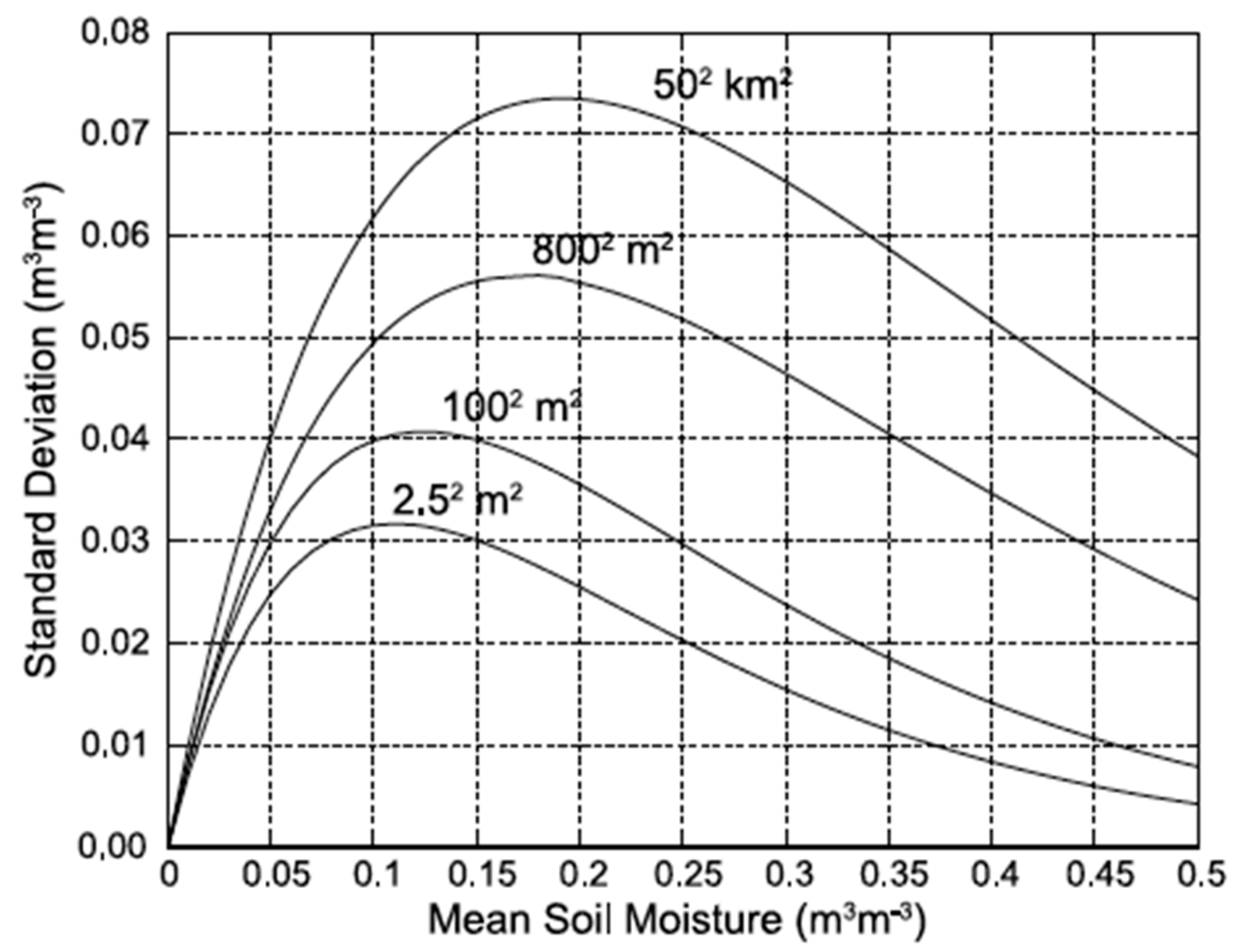
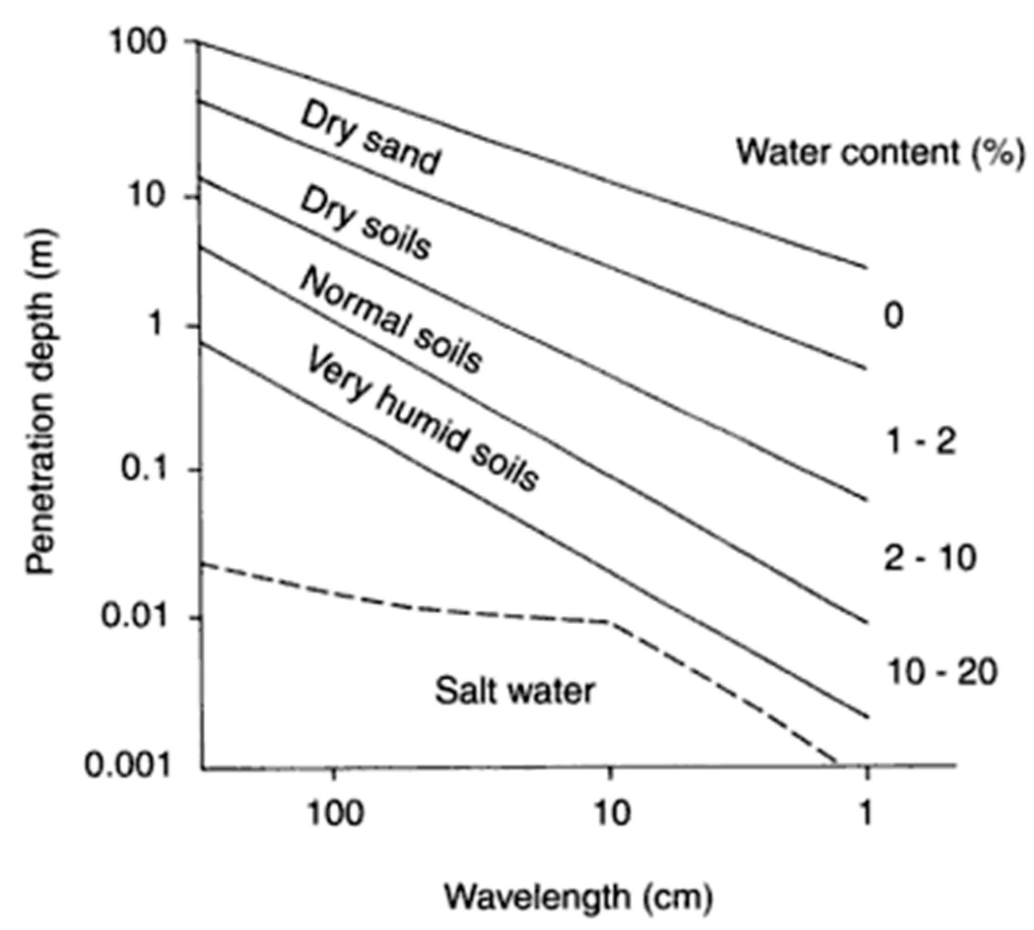
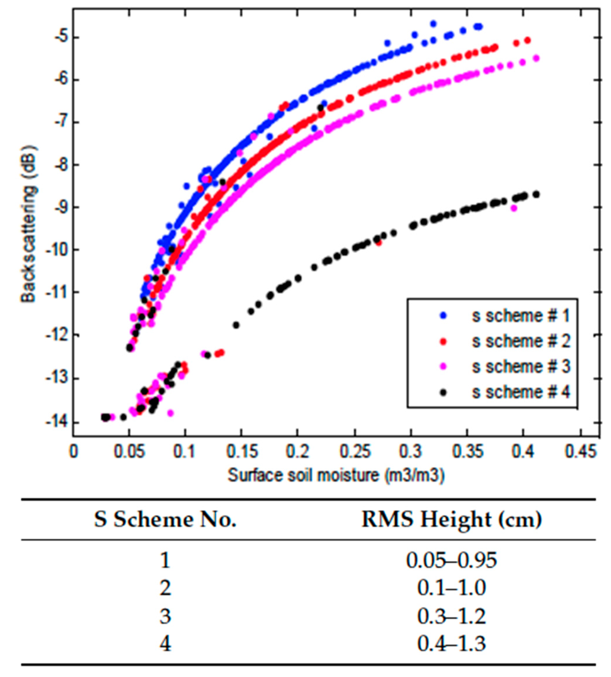
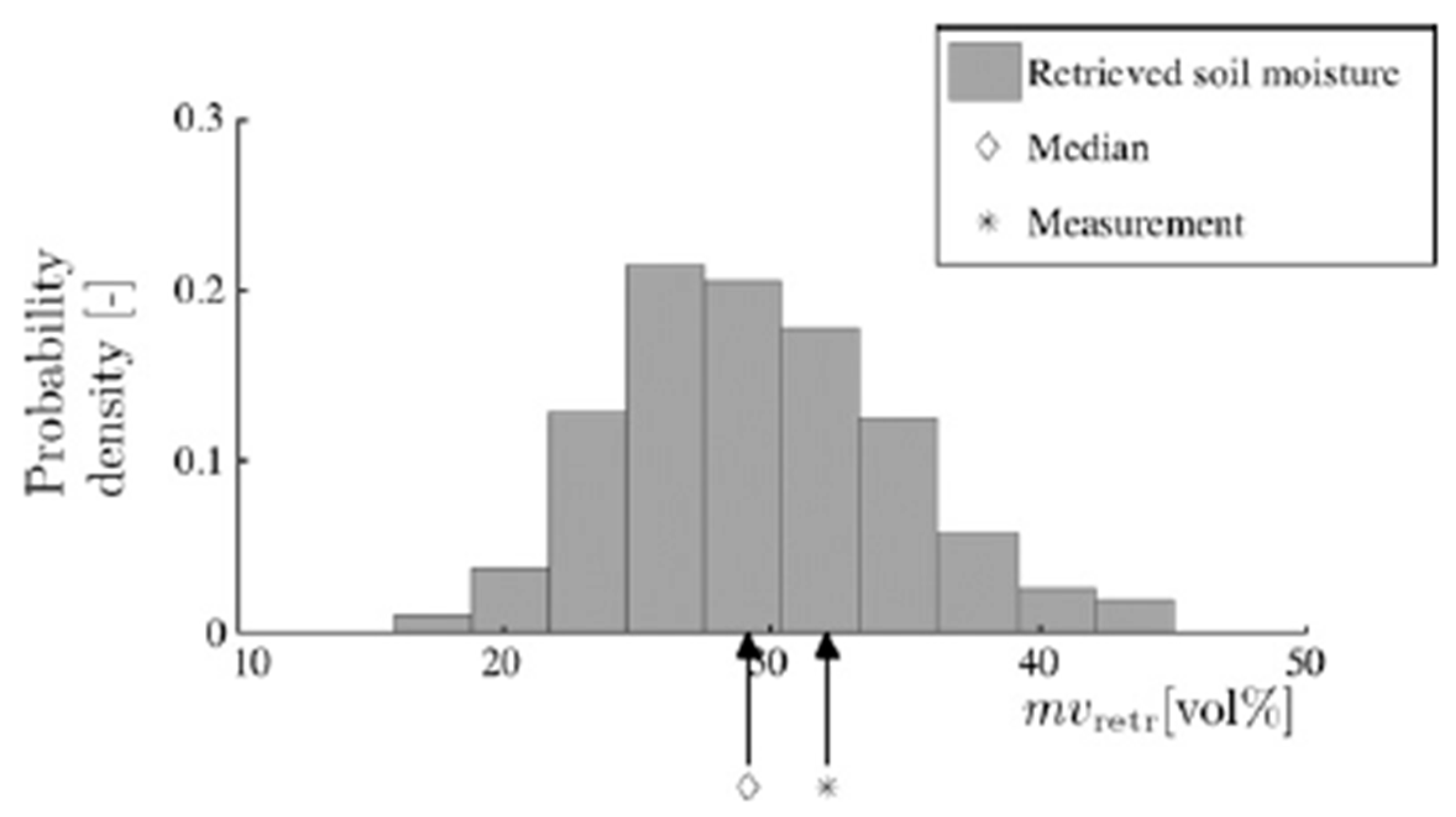
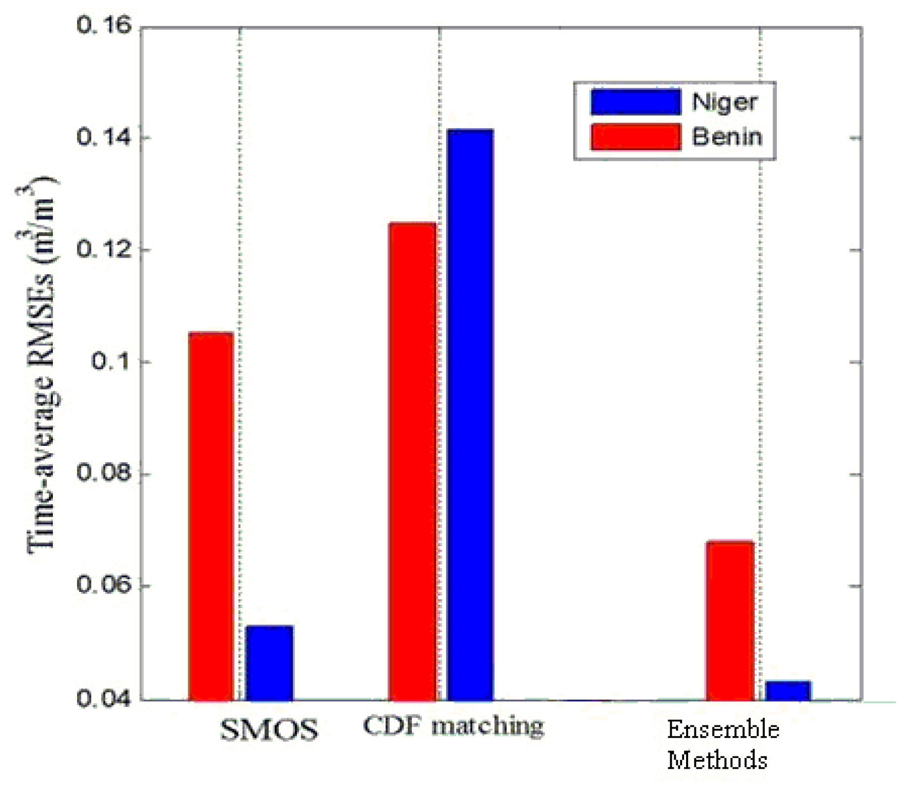
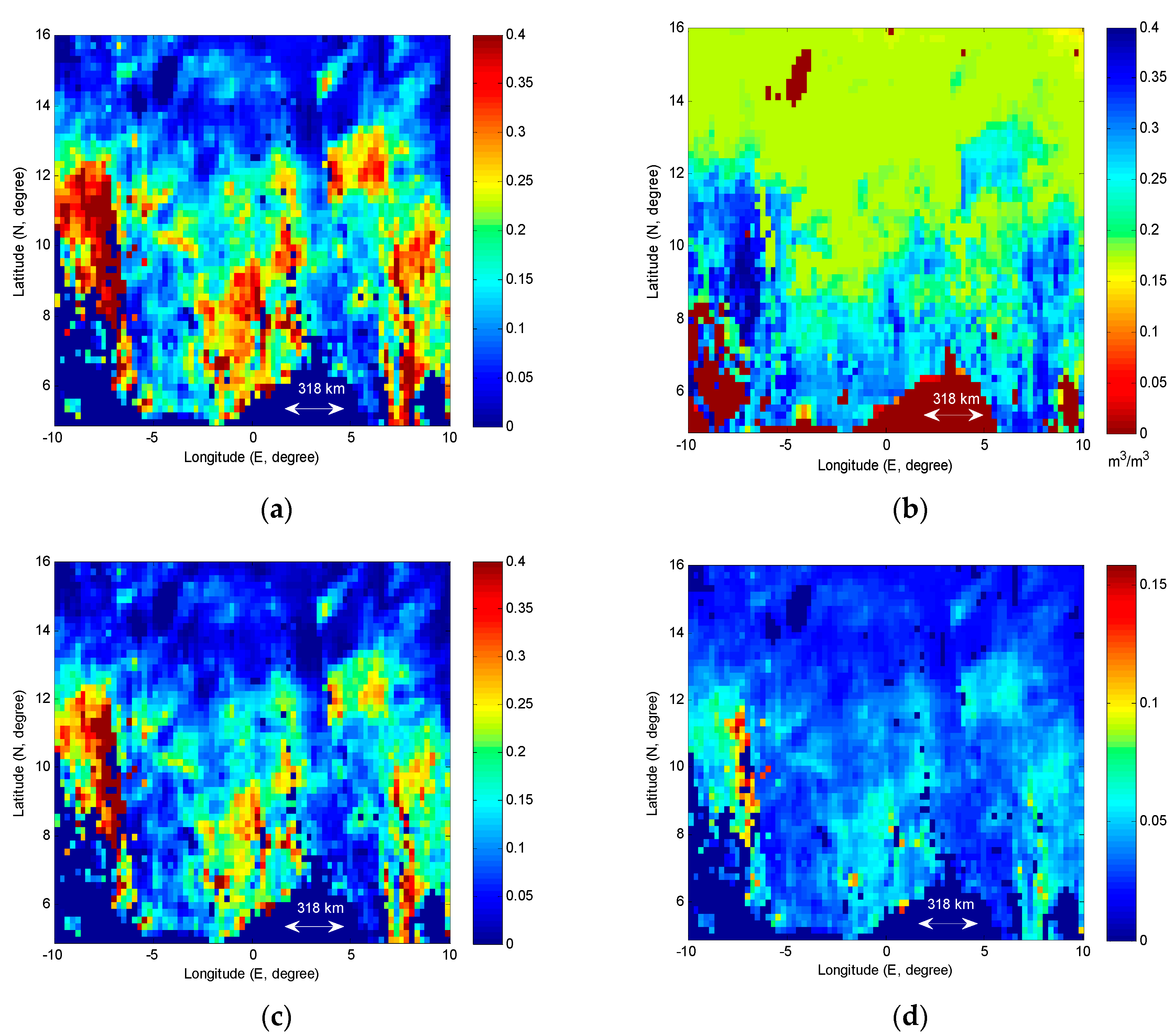
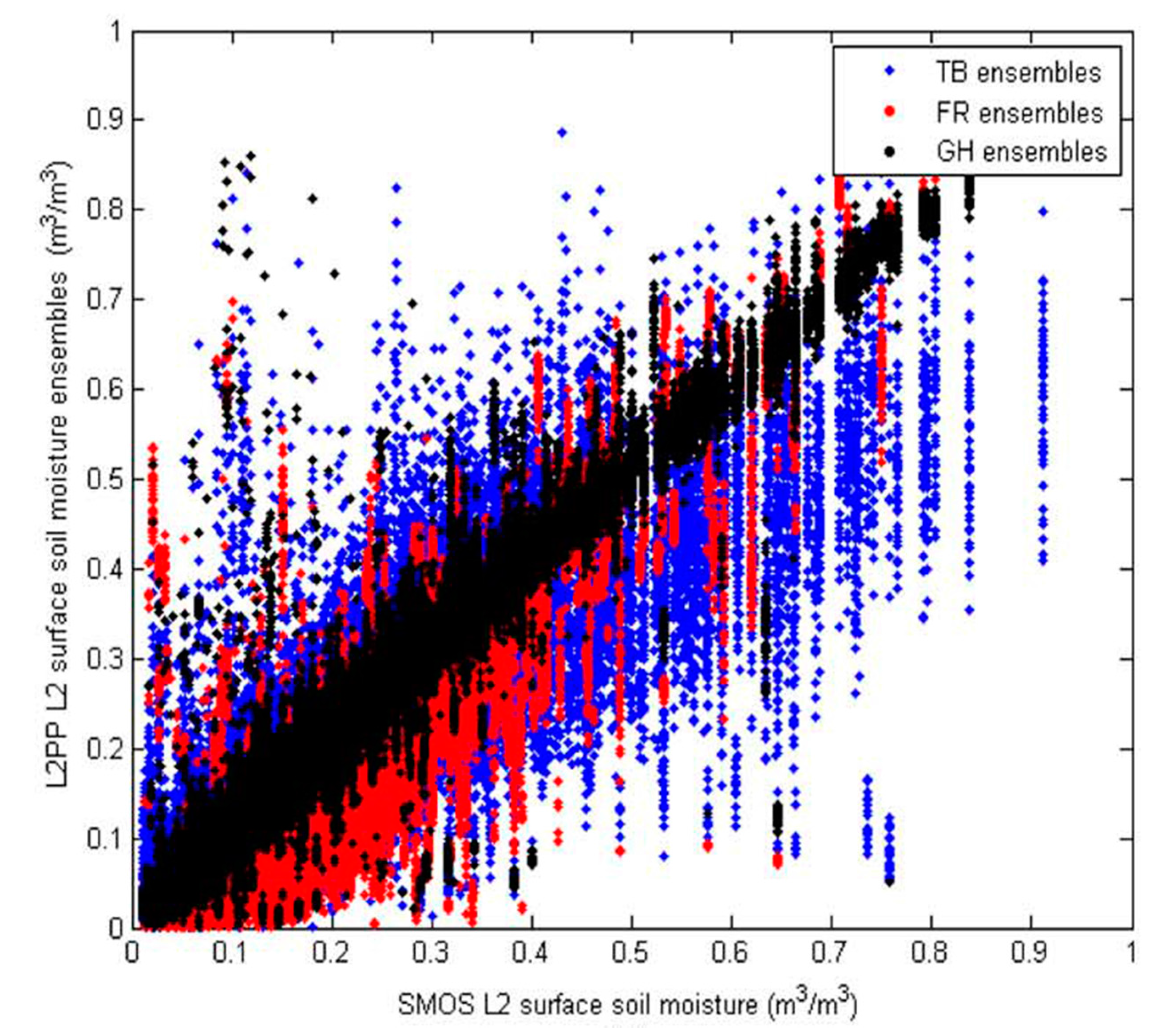
Table 1.
Error sources to consider for ensemble generation.
| Error Sources | Details | Error Range | Reference |
|---|---|---|---|
| Instrument measurements (backscattering/brightness temperature) | calibration error, incidence angle, interpolation error, RFI, instrument noise, topography, rainfall events, surface conditions | 20~30 K (e.g., ±10 K) | Lee et al. [30], de Rosnay [69], Lee and Im [52], Muñoz-Sabater [54] |
| 0.3~2.5 K | Crow et al. [59], Parinussa et al. [36] | ||
| 0.5~2 dB | Mattia et al. [70] | ||
| Geo-physical parameters | soil roughness, optical density, soil property, single scattering, albedo, surface temperature, vegetation coefficients, soil temperature | 6~10% | Verhoest et al. [16], Schmugge et al. [71] |
| 25~40 K | Holmes et al. [72] | ||
| −5~18 K | Schlenz et al. [73] | ||
| 20~30 K | Crow et al. [59] | ||
| Sub-pixel soil/land cover | land cover, mixing regime, soil map or vegetation fraction misclassification | 22~60% | Leroux et al. [45], Panciera et al. [74] |
© 2017 by the authors. Licensee MDPI, Basel, Switzerland. This article is an open access article distributed under the terms and conditions of the Creative Commons Attribution (CC BY) license (http://creativecommons.org/licenses/by/4.0/).
Share and Cite
MDPI and ACS Style
Lee, J.H.; Zhao, C.; Kerr, Y. Stochastic Bias Correction and Uncertainty Estimation of Satellite-Retrieved Soil Moisture Products. Remote Sens. 2017, 9, 847. https://0-doi-org.brum.beds.ac.uk/10.3390/rs9080847
AMA Style
Lee JH, Zhao C, Kerr Y. Stochastic Bias Correction and Uncertainty Estimation of Satellite-Retrieved Soil Moisture Products. Remote Sensing. 2017; 9(8):847. https://0-doi-org.brum.beds.ac.uk/10.3390/rs9080847
Chicago/Turabian StyleLee, Ju Hyoung, Chuanfeng Zhao, and Yann Kerr. 2017. "Stochastic Bias Correction and Uncertainty Estimation of Satellite-Retrieved Soil Moisture Products" Remote Sensing 9, no. 8: 847. https://0-doi-org.brum.beds.ac.uk/10.3390/rs9080847
Note that from the first issue of 2016, this journal uses article numbers instead of page numbers. See further details here.