Detection of Asian Dust Storm Using MODIS Measurements


1
School of Geography and Remote Sensing, Nanjing University of Information Science & Technology, Nanjing 210044, China
2
Institute of Remote Sensing and digital Earth, Chinese Academy of Sciences, Beijing 100101, China
3
Environmental Science and Technology Center (ESTC) and Department of Geography and GeoInformation Science (GGS), George Mason University, Fairfax, VA 22030, USA
*
Author to whom correspondence should be addressed.
Remote Sens. 2017, 9(8), 869; https://0-doi-org.brum.beds.ac.uk/10.3390/rs9080869
Submission received: 30 June 2017
/
Revised: 17 August 2017
/
Accepted: 19 August 2017
/
Published: 22 August 2017
(This article belongs to the Section Atmospheric Remote Sensing)
Abstract
:Every year, a large number of aerosols are released from dust storms into the atmosphere, which may have potential impacts on the climate, environment, and air quality. Detecting dust aerosols and monitoring their movements and evolutions in a timely manner is a very significant task. Satellite remote sensing has been demonstrated as an effective means for observing dust aerosols. In this paper, an algorithm based on the multi-spectral technique for detecting dust aerosols was developed by combining measurements of moderate resolution imaging spectroradiometer (MODIS) reflective solar bands and thermal emissive bands. Data from dust events that occurred during the past several years were collected as training data for spectral and statistical analyses. According to the spectral curves of various scene types, a series of spectral bands was selected individually or jointly, and corresponding thresholds were defined for step-by-step scene classification. The multi-spectral algorithm was applied mainly to detect dust storms in Asia. The detection results were validated not only visually with MODIS true color images, but also quantitatively with products of Ozone Monitoring Instrument (OMI) and Cloud Aerosol Lidar with Orthogonal Polarization (CALIOP). The validations showed that this multi-spectral detection algorithm was suitable to monitor dust aerosols in the selected study areas.

1. Introduction
The study of atmospheric aerosols has become a very interesting topic in recent years due to evidence showing their impact on climate change [1]. Aerosols, deserving of the same consideration as greenhouse gases, play important roles in atmospheric chemistry, cloud microphysics, temperature, and radiation balance in the lower atmosphere [2]. Dust storms are one kind of frequently occurring natural phenomena over the continents, which may have potential impacts on the climate, environment, and air quality. Dust storms, usually occurring in arid and semi-arid regions, can carry large quantities of dust and move forward like an overwhelming tide to destroy crop plants, ruin mining and communication facilities, weather vestiges, damage small villages, reduce visibility, and hinder human daily activities, as well as impact aircraft and road transportation. It pollutes the atmosphere and air quality, influences cloud formation [3], obscures sunlight, and alters temperature. Some dust storms can remain suspended in the air for several days and travel by wind far from where they originated. Recently, several studies have observed that heavy dust storms can impact the formation and evolution of hurricanes [4,5].
The detection of dust storms in a timely manner can serve as warnings for people to avoid economic loss and even loss of life. The detection results are also very useful for atmospheric modeling and simulation. Due to the large coverage of each dust storm, satellite remote sensing technology has been applied to detect and monitor dust storms. Color imagery techniques have been the primary tools used for dust storm monitoring in the past, where early researchers used the visible spectrum to monitor dust outbreaks as well as to estimate dust optical depth over oceanic regions [6,7]. Dust was detected and its evolution followed by its yellow color on Sea-viewing Wide Field-of-view Sensor (SeaWiFS) satellite images. Miller [8] applied color enhancement techniques to differentiate dust, ocean surfaces, and clouds. Several studies have also shown that it is possible to detect Saharan dust over land using brightness temperature (BT) in thermal infrared spectra [9,10,11,12]. A correlation of the BT between 11 µm and 3.7 µm bands for dust outbreaks was proposed by Ackerman [13], who developed a further tri-spectral (8, 11, and 12 µm) technique for detecting dust over water and for distinguishing dust plumes from water/ice clouds [14].
Currently, several approaches have been developed for dust storm detection using MODIS measurements given its good spectral, spatial, and temporal resolutions. Qu et al. [15] used the Normalized Difference Dust Index (NDDI), a normalized ratio of the 2.1 µm band and blue band, to detect dust storms and monitor the moisture change of the dust storm. NDDI has advantages due to the high sensitivity of the MODIS 2.1 µm band to moisture content. Hao et al. [16] proposed a thermal infrared index to detect Saharan dust storms by combining four moderate resolution Imaging Spectroradiometer (MODIS) thermal emissive bands (TEBs). An automatic multi-spectral approach for detecting dust storms in Northwest China was developed by Han et al. [17], where a set of indices was used to separate the dust from cloud, snow, and land with several Reflective Solar Band (RSBs) measurements.
However, most of abovementioned methods detect dust storms only with measurements of either RSBs or TEBs. Furthermore, the cloud mask product [18] is used directly, which may misclassify partial dust as clouds under some conditions, hence decreasing detection quality. In this paper, an algorithm based on the multi-spectral technique was developed, combining measurements of six MODIS RSBs and TEBs. The bands were selected according to the spectral analysis and the thresholds of each test were decided with the statistical analysis. Several dust storm events were selected as case studies to test the algorithm. Additionally, the results were validated not only with MODIS true color images, but also quantitatively with OMI and CALIOP measurements.
2. Data and Methods
2.1. Data
2.1.1. Moderate Resolution Imaging Spectroradiometer (MODIS)
MODIS, one of the key sensors of the NASA Earth Observing System (EOS), was launched onboard the Terra spacecraft on 18 December 1999 and the Aqua spacecraft on 4 May 2002 [19,20]. Both Terra and Aqua MODIS operate in a sun-synchronous orbit at an altitude of 705 km. Terra descends southwards with the local equatorial crossing time 10:30 a.m. and Aqua ascends northwards with the local equatorial crossing time 1:30 p.m. respectively. The MODIS makes Earth observations using 36 bands, including 20 RSBs and 16 TEBs with a wavelength range from 0.4 to 14.2 μm. Three different spatial resolutions have been designed based on the band specifications and science applications: 250 m (bands 1–2), 500 m (bands 3–7), and 1 km (bands 8–36). Among these bands, band 1 (red), band 4 (green), and band 3 (blue) are usually used for constructing RGB (Red Green Blue) true color images. The MODIS is a cross-track scanning radiometer with a two-sided scan mirror which rotates over a scan angle range of ±55°, producing a swath of 2330 km in scan direction and 10 km in track direction with each scan [21].
The MODIS L1A geolocation and L1B calibrated radiance dataset were used for detecting dust aerosols. The Aerosol Optical Depth (AOD) used in this paper was a level-2 C006 aerosol product, with a resolution of 10 km (at nadir), obtained from the Level 1 and Atmosphere Archive and Distribution System (LAADS) server https://ladsweb.modaps.eosdis.nasa.gov/. Table 1 shows the spectral bands of MODIS (Source: http://modis.gsfc.nasa.gov/about/specifications.php).
To accurately decide the bands and thresholds in the dust storm detection algorithm, more than fifty dust storm events in China that occurred during 2001–2007 (2001–2007 for Terra MODIS and 2002–2007 for Aqua MODIS) were collected as training data for spectral analysis. Detailed information of each selected dust storm event is listed in Table 2, including the sensor, year, day, and UTC (Coordinated Universal Time) time. Cloud pixels and clear pixels were also collected, and are presented in Table 3 and Table 4, based on the MODIS cloud mask product.
2.1.2. Ozone Monitoring Instrument (OMI)
OMI was also onboard Aura. OMI views the Earth with a wide view angle of ±57° relative to the nadir. The large swath (up to 2600 km in scan direction) enables OMI to achieve almost daily global coverage in 14 orbits [22,23]. OMI was designed for monitoring the ozone and other atmospheric species including aerosols, and is a hyperspectral sensor that observes solar backscatter radiation in the ultraviolet (UV) and visible spectrum (range from 270 nm to 500 nm) at a spectral resolution of about 0.5 nm [23,24].
The wavelengths and algorithms used for retrieving OMI aerosol parameters are significantly different from those of MODIS. These differences do produce some advantages, such as the high sensitivity of the OMI UV retrieval algorithm to aerosol absorption and the ability to retrieve aerosol information over bright surfaces and clouds [25]. The OMI Ultra Violet Aerosol Index (UVAI) is an effective index to reflect the presence of absorbing aerosols. Therefore, a UVAI product was adopted for the quantitative validation of dust detection derived from MODIS measurements. The UVAI product can be obtained from Goddard Earth Sciences Data and Information Services Center (GES DISC) server at http://disc.sci.gsfc. nasa.gov/SSW/.
2.1.3. Cloud-Aerosol Lidar with Orthogonal Polarization (CALIOP)
CALIOP, on board Cloud-Aerosol Lidar and Infrared Pathfinder Satellite Observation (CALIPSO), was launched on 28 April 2006. It flies along the same orbit as the Aqua spacecraft and is 1 min and 15 s behind. CALIOP is a two-wavelength polarization-sensitive Lidar that is designed to acquire the vertical profiles of aerosols with a backscatter signal at 532 nm and 1064 nm both day and night, as well as profiles of linear depolarization at 532 nm [26]. The Vertical Feature Mask (VFM)—one of the CALIOP level 2 products—provides scene classification in a 16-bit integer for each altitude resolution element. The VFM classifies various scene features into several types such as clear air, cloud, aerosol, surface, and so on. Based on these types, it can separate airborne dust from ground dust with the vertical information of aerosol and cloud layers. Therefore, the CALIOP VFM was used to validate the dust detection derived with MODIS measurements, and can be obtained from the Atmospheric Science Data Center (ASDC) server at https://eosweb.larc.nasa.gov/JORDER/ceres.html.
2.2. Methodology
2.2.1. Algorithm Development
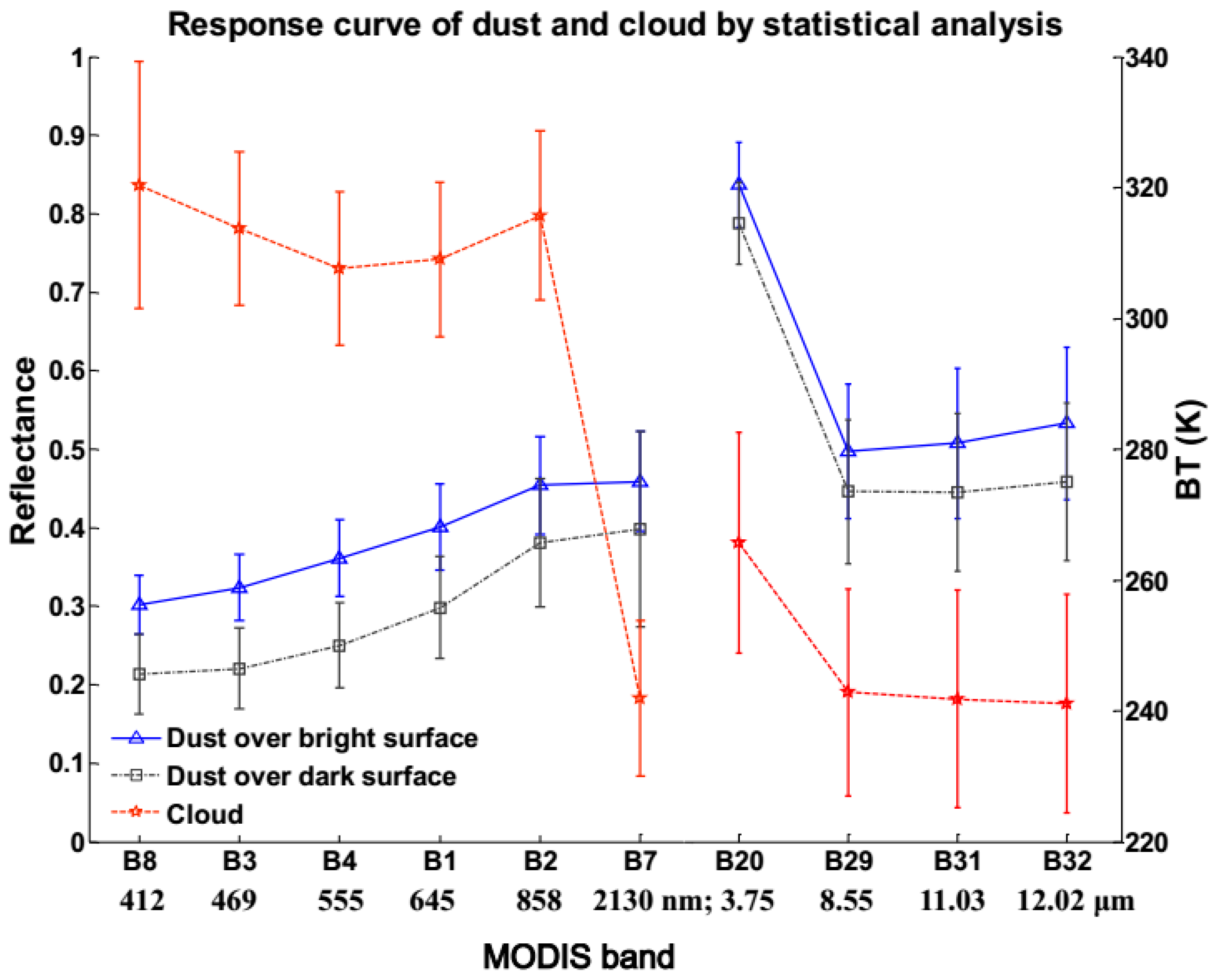
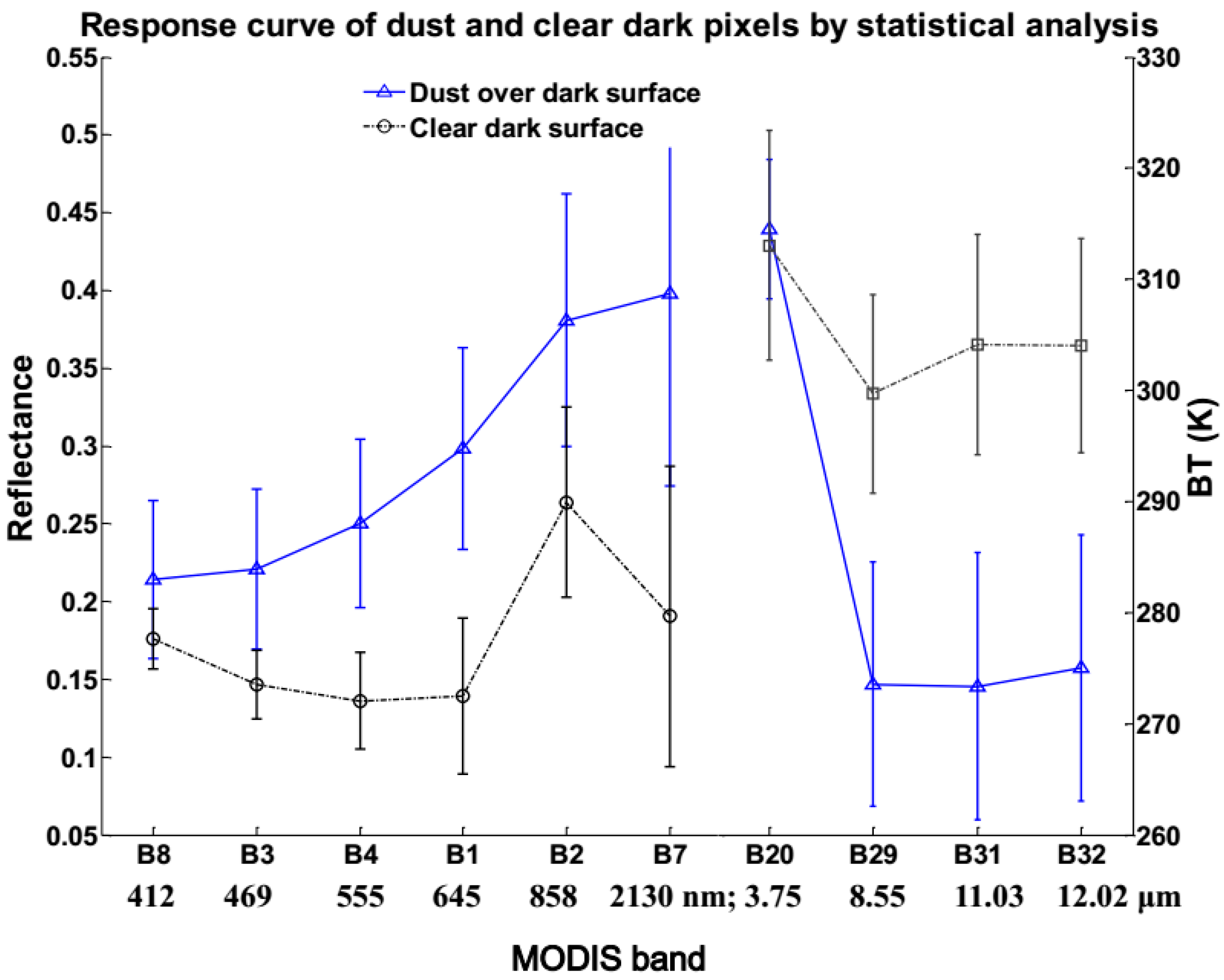
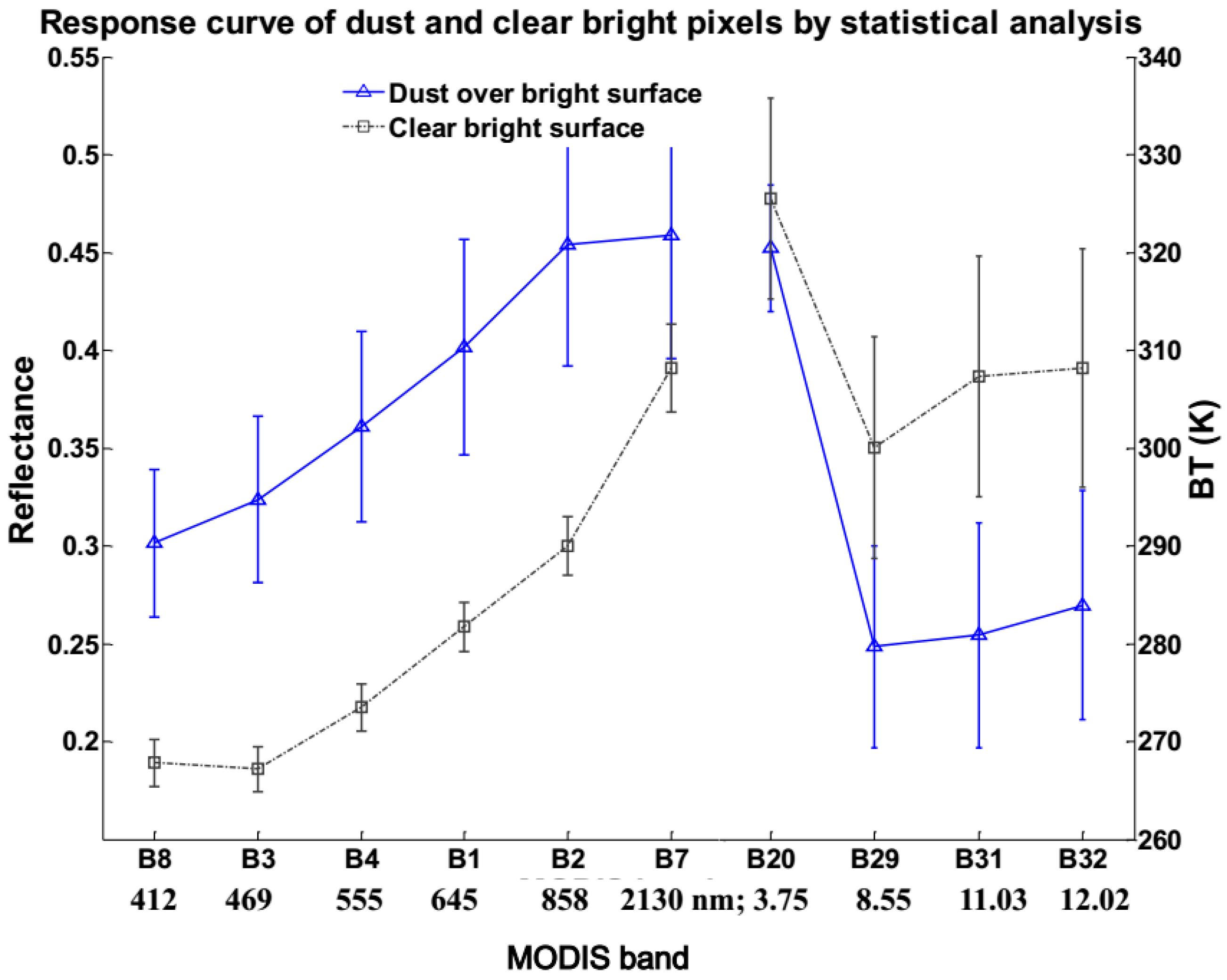
According to selected cases, most Asian dust storms originate and dissipate within inland areas. Therefore, the training data of dust events (shown in Table 2) can be roughly divided into two categories by underlying land surface type: dust storm over bright surface, or over dark surface. The spectral curves of these two categories of dust storms are shown in Figure 1, as well as clouds. Figure 2 and Figure 3 represent the spectral curve comparisons between dust and clear conditions over dark and bright surfaces separately. The spectral response at each band is the statistical mean value of all training data, as well as the standard deviation.
In Figure 1, cloud shows a high reflectivity in band 3 (469 nm) and a low reflectivity in band 7 (2130 nm), while dust displays a reverse trend. In the thermal spectrum, cloud had a much lower brightness temperature than dust. This difference assists their separation significantly. In Figure 2 and Figure 3, the relatively large response difference between the dust and clear scenes over both dark and bright surfaces was found at band 1 (red band 645 nm). Additionally, the Bright Temperature Difference (BTD) (3.7, 11) value of dust was larger than that of clear scenes.
In Figure 1, the brightness temperature in the thermal spectrum between dust and cloud was obviously different. Ackerman [14] proposed an IR split windows technique to discriminate the dust storm layer from cloud using the brightness temperature difference between the 11 and the 12 μm regions of the spectrum. Based on Ackerman’s conclusion, the BTD (12, 11) value was negative for cloud and positive for dust. Meanwhile, the spectral curves in Figure 1 exhibited the same characteristics. Furthermore, dust had a high reflectivity at band 7, but a low reflectivity at band 3 (blue band 469 nm). In contrast, the blue band was sensitive to cloud, but band 7 was insensitive to cloud. These inverse spectral features greatly helped to distinguish between dust and cloud.
Qu et al. [15] raised a Normalized Difference Dust Index (NDDI) to detect dust, with the formula NDDI = (R3 − R7)/(R3 + R7), and the BTD (3.7, 11) was selected to separate dust from surface scenes. From Figure 2 and Figure 3, we can see that both dust and surface scenes had a similar BT at band 20 (3.7 μm), but dust had a much lower BT at the thermal spectrum than surface scenes. Additionally, the BTD of band 31 (11 μm) relative to band 20 had the largest statistical difference between dust and surface scenes. Moreover, in a reflective solar spectrum, the relative large reflectance difference between the dust and surface scenes (both bright and dark surfaces) was found at band 1. Therefore, the single reflectance of band 1 was picked up to differentiate dust from surface scenes.
Overall, the BTD (12, 11) and NDDI were chosen to discriminate between dust and cloud, while the BTD (3.7, 11) and the single reflectance of band 1 were chosen to identify dust over both dark and bright surfaces.
2.2.2. Training Process and Flowchart
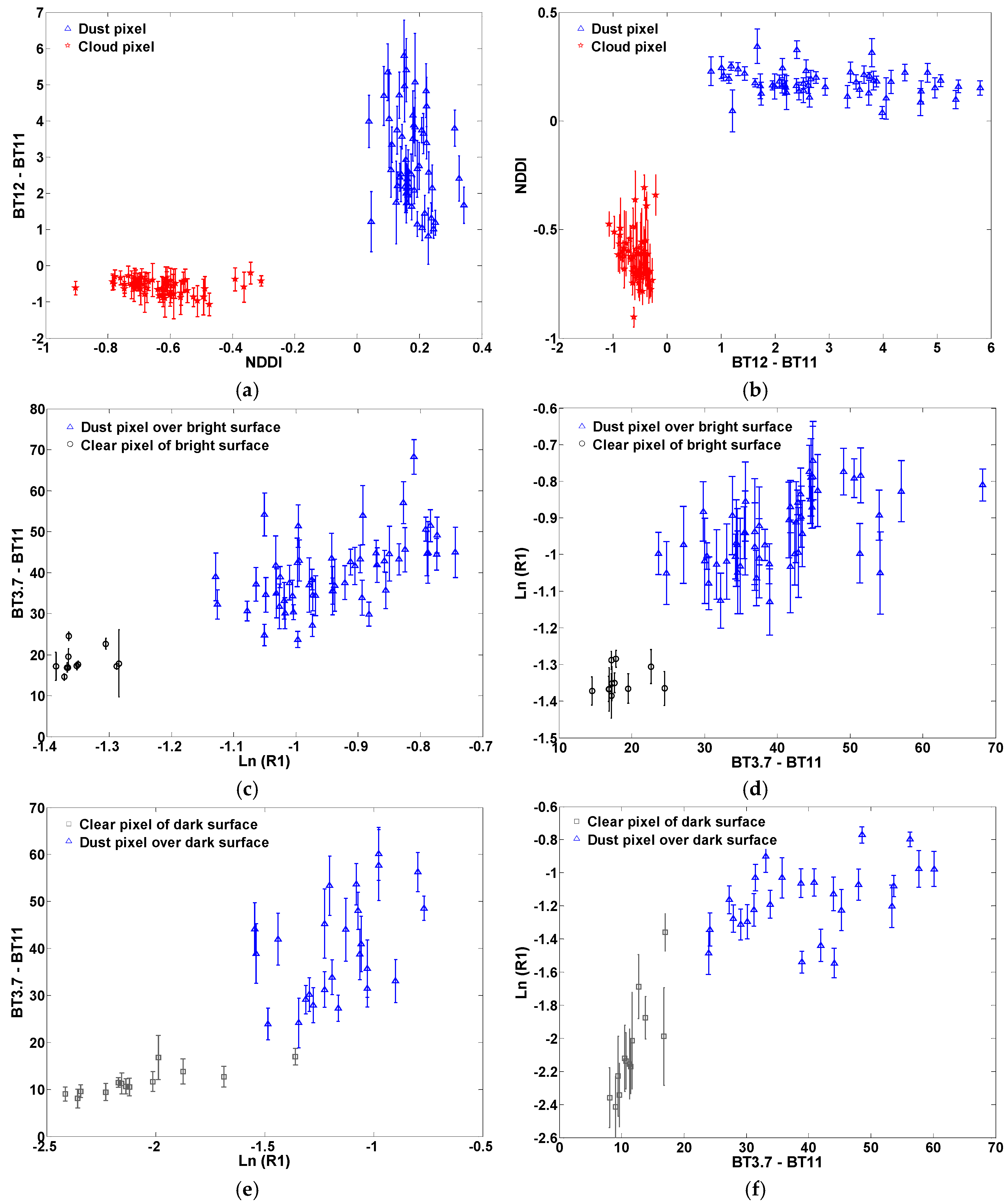
Based on the above analysis, we chose four indices to detect dust: NDDI, BTD (12, 11), BTD (3.7, 11), and the logarithm of the single reflectance of band 1. To determine the thresholds of the four indices, we calculated and tested all training data. Figure 4 shows the scatterplot of the four indices separately, in which each data point was the average value of one dust storm event, along with the standard deviation.
Figure 4a,b show a large difference in the NDDI and BTD (12, 11) values between cloud and dust. Clearly, cloud had negative BTD (12, 11) and NDDI values, while in contrast, dust had positive values of these two indices. Meanwhile, dust had larger BTD (3.7, 11) values than clear bright surfaces (Figure 4c) and clear dark surfaces (Figure 4e). Among them, the BTD (3.7, 11) values of the dark surface was smallest, generally less than 20 K. In Figure 4d,f, the logarithm of the single reflectance of the red band was introduced to separate dust from surface scenes. This indicated that using logarithm could enhance the resolving power of this index, especially in a small reflectance range. Obviously, the Ln (R1) of most dust pixels was larger than −1.2 over bright surfaces, and −1.6 over dark surfaces.
The detailed thresholds of each index are summarized in the Table 5. It should be noted that the errors listed in Table 5 represent (when using the corresponding thresholds to determine dust or cloud) the percentage of misclassified pixels. The largest error appeared at the separation of dust from cloud over dark surfaces in the reflective solar spectrum, which was up to 12.5%. This large error was possibly caused by light dust pixels suspended over water. Considering that some pixels could be counted repeatedly, the total errors of both over bright and dark surfaces were not equal to the summation of the errors from each test.
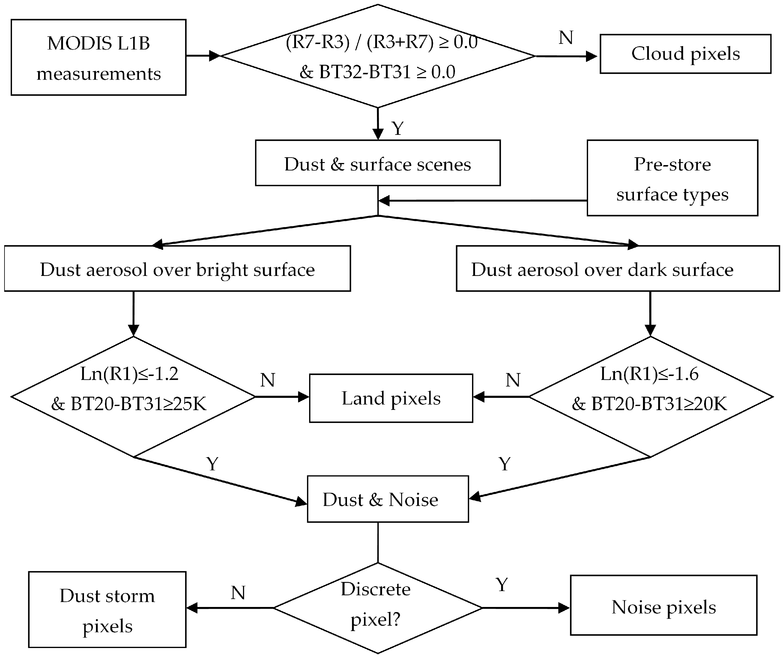
Based on the above analysis and the thresholds listed in Table 5, an algorithm based on the multi-spectral technique for detecting dust aerosol was developed. The flowchart of this dust detection algorithm is shown in Figure 5. First, the MODIS L1B measurements were input into the cloud module to filter out cloud by employing BTD (12, 11) and NDDI. Next, the remaining pixels were divided into two branches based on pre-stored surface type information: dust over bright surfaces and over dark surfaces. Third, the BTD (3.7, 11) and the logarithm of reflectance at band 1 were applied in both branches with respective thresholds. At the end of the process, an additional test was executed to further filter out discrete pixels. In view of the dust continuity, if a pixel was identified as a dust pixel but was not close to other dust pixels, this pixel was considered as noise and deleted from the dust images. It should be noted that since dust aerosol detection is based on the MODIS measurements pixel by pixel, the spatial resolution of dust aerosol detection results was up to 1 km.
3. Results and Discussion
In this section, we conducted the dust storm detection test with MODIS RSB and TEB measurements based on the algorithm shown in Figure 5. Furthermore, the quantitative validation of the dust detection results with OMI and CALIOP was also executed.
3.1. Algorithm Test Cases
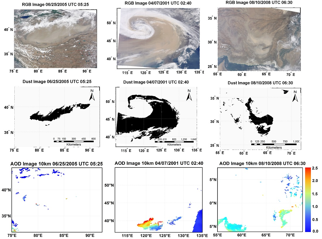
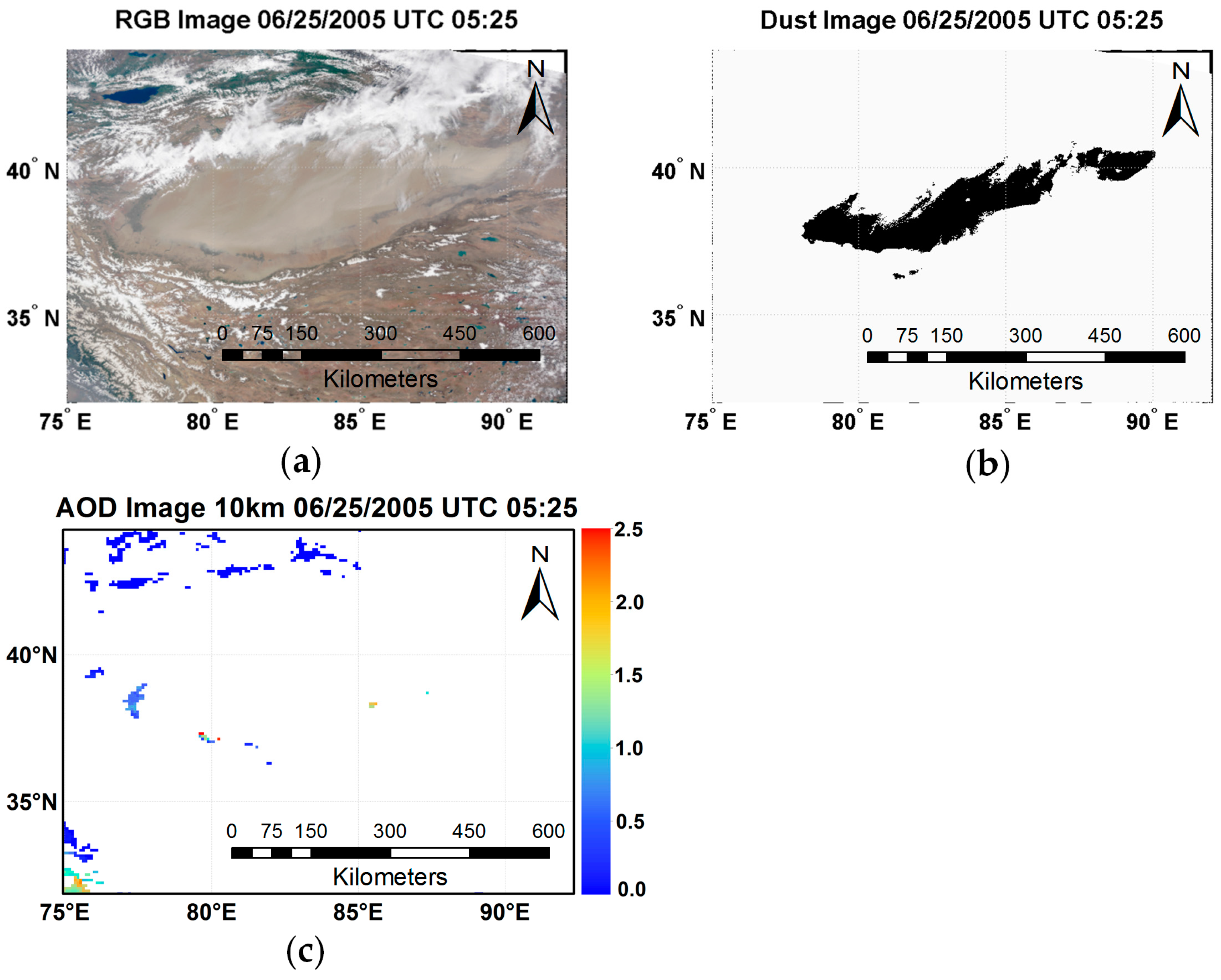
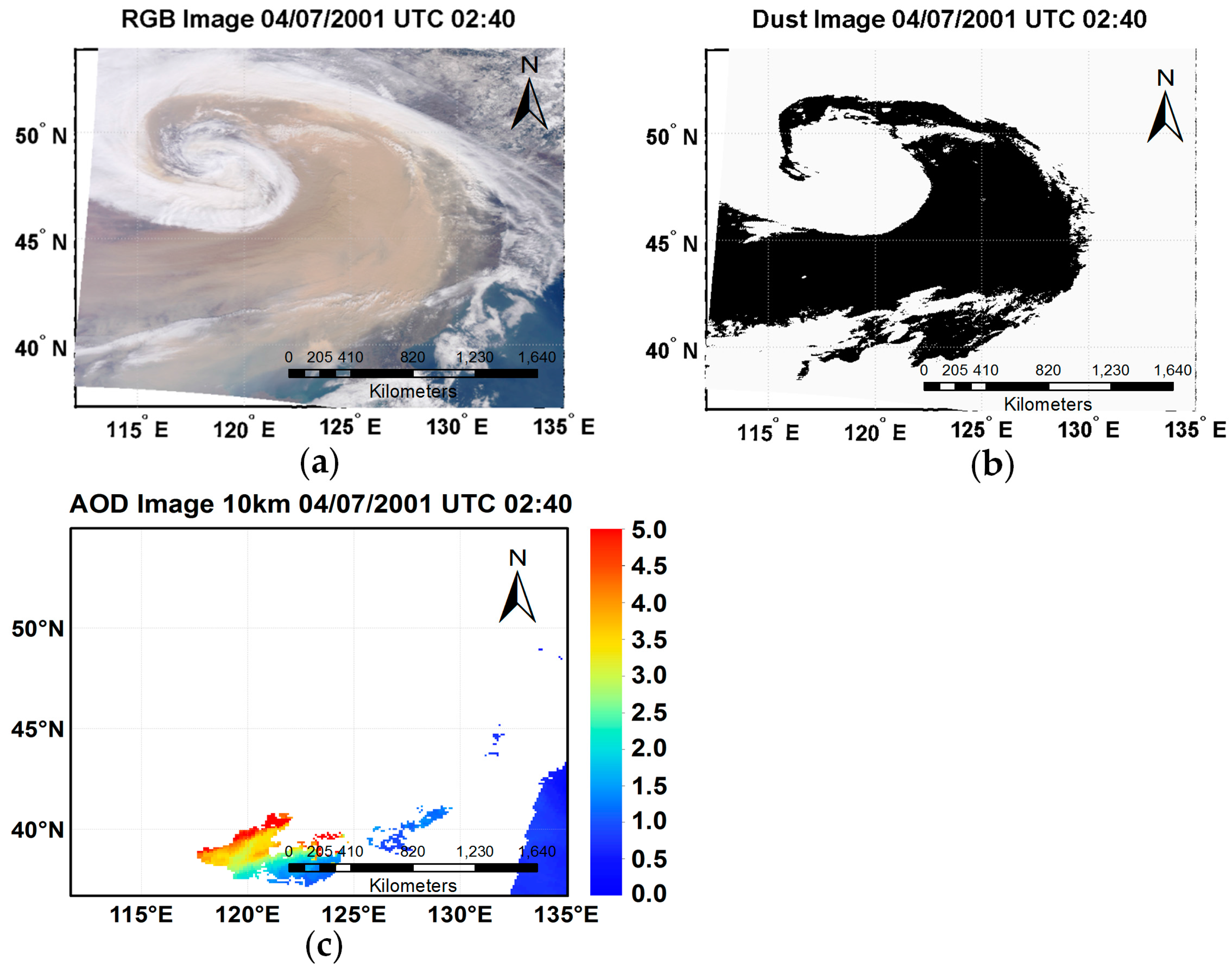
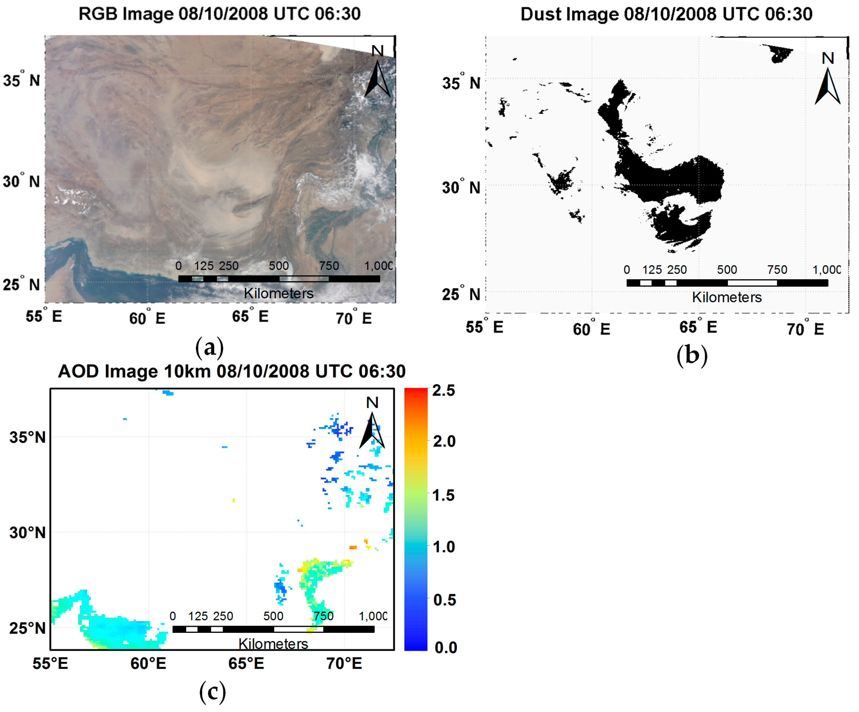
We selected three MODIS measurements to represent the dust events occurring in different locations, the results of which are shown in Figure 6, Figure 7 and Figure 8, respectively. Figure 6 represents the dust storm above the Taklimakan Desert, captured by Terra MODIS on 25 June 2005. From Figure 6a (MODIS true color image), we can see that the dust storm was blown in a long, narrow shape, while in Figure 6b the detected dusts were marked with a black color, which had good agreement with the MODIS true color image. The dust in Figure 7 was a large dust storm that covered most of Northeastern China, captured by Terra MODIS on 7 April 2001. It is worth noting that the dust storm was mixed with cloud, clearly shown in Figure 7a. Nevertheless, in Figure 7b, the dust pixels were obviously separated from the cloud through a comparison with the MODIS true color image. This indicated that our multi-spectral dust detection technique could distinguish between dust and cloud extremely well. Only a small part of dust aerosol pixels over the ocean (left bottom corner) was missed as the algorithm mainly focuses on the land area. In Figure 8, the dust storm spread across two countries, Pakistan and Afghanistan, on 10 August 2008. Two strings of dust plumes in the middle of the image were identified successfully, and another small dust storm in the right upper corner was also detected.
The MODIS Aerosol Optical Depth (AOD) images in the same region were displayed for comparison, as shown in Figure 6c, Figure 7c, and Figure 8c. In the AOD images, the AOD was not accurately retrieved for the areas with heavy dust loading as the aerosol inversion algorithm taken by the MODIS usually failed to retrieve AOD when there was a high concentration of aerosols [27]. Therefore, in this condition, the detecting results of the algorithm described in Figure 5 could provide more accurate information about the dust aerosols than the MODIS AOD product.
3.2. Validation of Dust Storm Detection with OMI
The OMI instrument can distinguish between aerosol types such as smoke, dust, and sulfates. The UVAI is an index to measure how much the wavelength depends on the backscattered UV radiation as an atmosphere containing aerosols (Mie scattering, Rayleigh scattering, and absorption) differs from that of a pure molecular atmosphere (pure Rayleigh scattering). It is a qualitative indicator of the presence of the absorbing aerosols, defined as UVAI = −100 log10 (I360Meas/I360Calc), where I360Meas is the measured 360 nm OMI radiance and I360Calc is the calculated 360 nm OMI radiance for a Rayleigh atmosphere [27,28]. Since the UVAI is only sensitive to absorbing aerosols, it is able to identify absorbing aerosols (such as dust) from weakly or non-absorbing particles. Usually, aerosols that absorb in the UV range yield positive UVAI values. Near-zero UVAI values appear when the sky is clear or there are large non-absorbing aerosols and clouds which have a nearly zero Angstrom coefficient. The non-absorbing small particle aerosols are the main source of negative UVAI values due to their non-zero Angstrom coefficients [29]. Hence, in this section the dust detection result was validated by OMI UVAI.
The Aqua MODIS measurements on 23 October 2007 at UTC time 04:55 were selected to conduct dust detection based on the multi-spectral dust detection technique illustrated in Section 2 (Figure 5). Figure 9a represents the MODIS true color image, which shows that a dust storm was raging in central China. Figure 9b shows the dust detection results. The UVAI values associated with dust aerosol are usually larger than 1.2, according to the procedure of aerosol selection in the OMAERUV README file. Therefore, only areas with UVAI values larger than 1.2 in the OMI UVAI image are shown in Figure 9c.
Validation was executed by matching pixels from two sensors (MODIS and OMI) with their geolocation measurements in the overlapping region. Table 6 shows the statistics of the difference between the dust detection results and the UVAI. With comparison, a total of about 187,472 pixels were labeled as dust with the OMI UVAI product. Among these pixels, 137,554 pixels (70.77%) were labeled as dust in the MODIS dust image, but 49,918 pixels (25.68%) were undetected. Furthermore, 6871 pixels (3.55%) were identified as dust in the MODIS dust image, but labeled as non-dust pixels in the OMI UVAI image. Figure 9d gives the spatial distribution of all identified, unidentified, and misidentified pixels and also shows that the center part of the dust storm was detected by both images (Figure 9b,c). The major difference existed at the edge of the dust storm, where many pixels were labeled as dust aerosol in the OMI UVAI image. This difference may be attributed to the different spatial resolutions between the two sensors. However, due to the different spatial resolutions, the number of dust pixels in the MODIS dust image (1 km) was not enough to aggregate a corresponding pixel in the OMI UVAI image (10 km). In other words, some dust pixels in the OMI UVAI image were not filled with dust pixels in the MODIS dust image. Statistically, at the margin area, more than 5% difference could be attributed to the spatial resolution differences between two sensors. Moreover, the small clouds that floated above the dust storm contributed another 3% of errors, which were too small to be detected by the OMI sensor.
3.3. Validation of Dust Storm Detection with CALIOP
CALIOP can separate airborne dust from ground dust with the vertical information of aerosol and cloud layers. The CALIOP VFM classifies various scene features into seven types: invalid (bad or missing data), clear air, cloud, aerosol, stratospheric feature (polar stratospheric cloud or stratospheric aerosol), surface, and no signal. These types can be used for the quantitative validation of dust detection results.
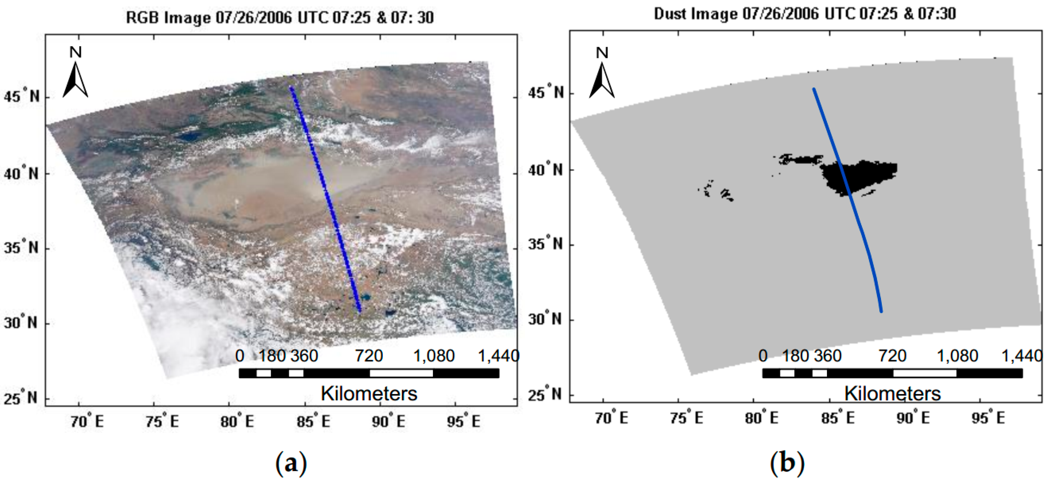
Aqua MODIS measurements over the Taklimakan Desert on 26 July 2006 were selected to conduct dust detection, based on the multi-spectral dust detection technique illustrated in Section 2 (Figure 5). Figure 10a shows the MODIS true color image, which was generated with measurements extracted from two swaths at the UTC times of 7:25 and 7:30. The dust aerosol was located in the eastern part of the desert. Meanwhile, the blue dash line represented the footprint of CALIOP in this area. Figure 10b shows the dust detection result and the footprint of CALIOP in the blue dash line. The VFM product of the region marked by the blue dash line is shown in Figure 11.
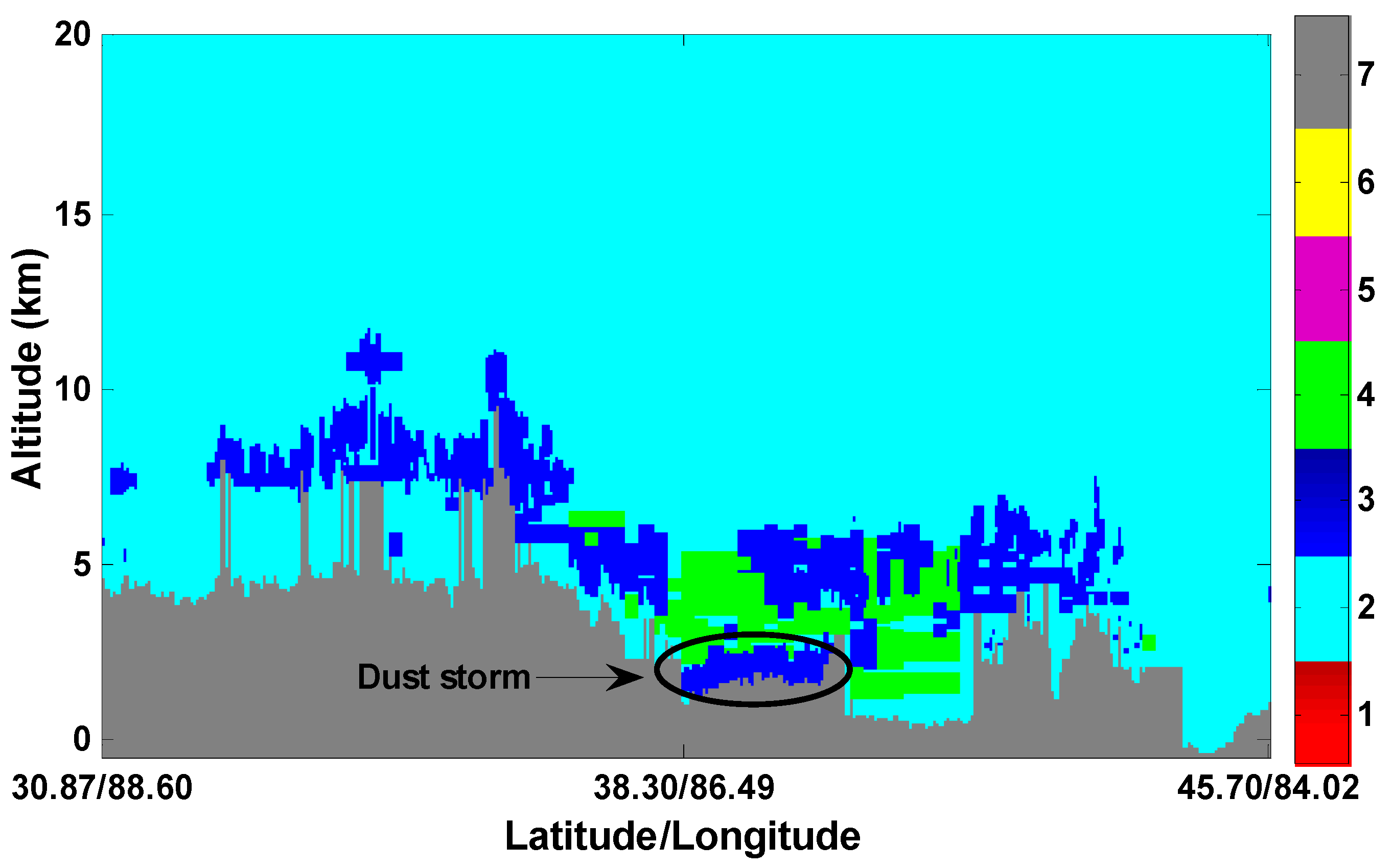
It is worth noting that the CALIOP VFM may misclassify dust aerosols as cloud, which is observed in Figure 11. The black circle represents the dust aerosol layer misclassified as cloud. To avoid the impact of misclassification (while considering the difference between VFM’s more than one vertical layer and MODIS’s single layer), we redefined the VFM types so that when dust was marked in one layer, the whole layer was recognized as dust. After the types were redefined, the pixels of CALIOP and MODIS were matched based on their geolocation.
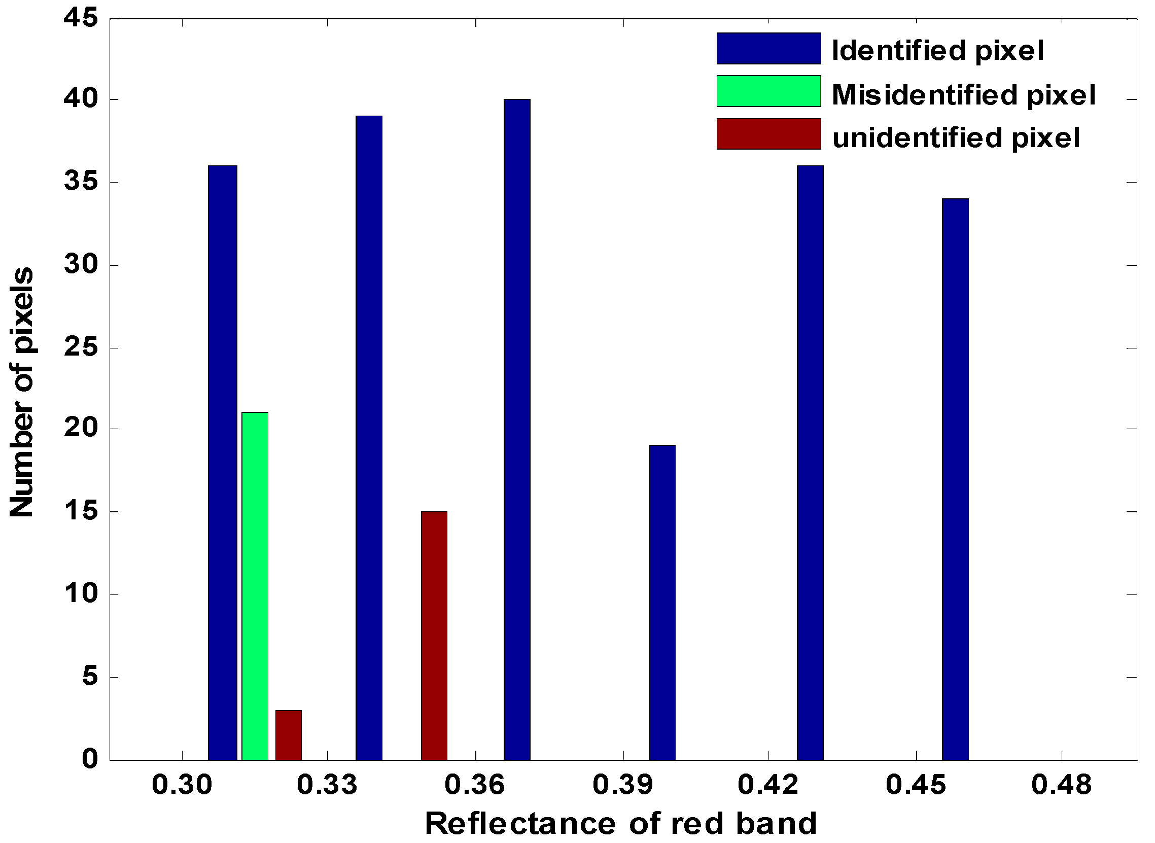
Error analysis was performed to count the number of pixels identified (pixels labeled as dust aerosols with both sensors), unidentified (pixels labeled as dust aerosols with only CALIOP, but undetected with MODIS), and misidentified (pixels labeled as non-dust aerosol pixels with CALIOP, but detected with MODIS). Generally, the stronger the dust storm, the higher reflectance in the red band. Therefore, the dust aerosol pixels were sorted into several categories according to their reflectance at the red band, as seen in Figure 12. There were 204 pixels identified and only 18 pixels unidentified. Approximately 91.89% of the dust aerosol pixels obtained from the proposed multi-spectral detection algorithm were correctly identified in a comparison with the CALIOP VFM data product. Additionally, there were 21 pixels misidentified. In reality, the statistical analysis showed that most of the heavy dust aerosol pixels were identified. Unidentified and misidentified dust aerosol pixels were mostly concentrated in the low reflectance range at the red band, namely low dust aerosol loading. Figure 13 displays the profile of the dust storm in the sensor motion direction using the reflectance at the red band. In Figure 13, the errors (unidentified or misidentified) were located only at the margin of the dust storm with light aerosol loading. Consequently, the multi-spectral algorithm of MODIS could be used for dust aerosol detection over a bright surface.
4. Conclusions
In this paper, a multi-spectral algorithm for observing and monitoring dust aerosols over both bright and dark surfaces was developed by combining measurements of the MODIS solar (RSB) and thermal bands (TEB).
The spectral curves of several major scene types, such as dust, cloud, vegetated surface, and non-vegetated surface, were derived statistically from a large quantity of training data. According to spectral analysis, the algorithm was divided into bright surface and dark surface branches for dust detection. In the algorithm, the thermal bands were mainly used for filtering out cloud, as well as a water vapor band, while the RSBs were selected for separating dust aerosols from other scene types. Well-developed indices from other previous studies were adopted directly, and some tests were proposed for the first time, including the reflectance of the red band used for dust detection. By comparing the MODIS true color image, the core part of the dust pixels was correctly identified, except for some missing pixels that had relatively low intensity. Meanwhile, OMI UVAI and CALIOP were selected for quantitative validation. The validation by OMI UVAI showed that most plumes (more than 70%) were detected. One main factor that impacted the accuracy of the algorithm may be attributed to the spatial resolution difference between the two sensors. The validation by CALIOP VFM showed that more than 90% of dust aerosol pixels were identified correctly in the selected case. Although there were some misclassified pixels, most of them were concentrated at the edge of the dust storm with light dust aerosol loading. Statistical analysis of the training data was the primary method used in this research to achieve the desired spectral features of the dust. Although the statistical analysis provided reasonable results, its accuracy was dependent on the number of training data. Moreover, the thresholds used in the algorithm were usually site-specific, which limited the application of the algorithm.
This approach for detecting dust aerosols with satellite remote sensing could be enhanced with further studies such as adding more precise site-specific information. Currently, the surface has only been separated into dark and bright surfaces for dust storm monitoring, thus a stricter classification of surface features and site-specific thresholds could enhance the accuracy of the algorithm significantly. It would be of great value to build a lookup table to store the site-specific thresholds for the entire global dataset. On the other hand, some useful research aims to be implemented based on this dissertation in the near future include: (1) tentative retrieving of the AOD based on the detection results; and (2) gathering dust information over a long time range. With long-term aerosol information, it is feasible to analyze their distribution, as well as their motion, height, width, and even seasonal variation.
Acknowledgments
This paper was supported by National Natural Science Foundation of China (No. 41501404); National Natural Science Foundation of China (No. 41671345); National Key Research Program of China (No. 2016YFB0502500); Scientific Research Foundation for the talent, Nanjing University of Information Science & Technology. The authors acknowledge data support from NASA and NOAA.
Author Contributions
Yong Xie designed the research, carried out the modeling, and prepared the manuscript. All authors contributed to the scientific content, the interpretation of the results, and manuscript revisions.
Conflicts of Interest
The authors declare no conflict of interest.
References
- Estellés, V.; Martínez-Lozano, J.A.; Utrillas, M.P.; Campanelli, M. Columnar aerosol properties in Valencia (Spain) by ground-based Sun photometry. J. Geophys. Res. Atmos. 2007. [Google Scholar] [CrossRef]
- Li, Z.; Khananian, A.; Fraser, R.H.; Cihlar, J. Automatic detection of fire smoke using artificial neural networks and threshold approaches applied to AVHRR imagery. IEEE Trans. Geosci. Remote Sens. 2001, 39, 1859–1870. [Google Scholar] [CrossRef]
- Kelly, J.T.; Chuang, C.C.; Wexler, A.S. Influence of dust composition on cloud droplet formation. Atmos. Environ. 2007, 41, 2904–2916. [Google Scholar] [CrossRef]
- Dunion, J.P.; Velden, C.S. The impact of the Saharan Air Layer on Atlantic tropical cyclone activity. Bull. Am. Meteorol. Soc. 2004, 85, 353–365. [Google Scholar] [CrossRef]
- Wu, L.; Braun, S.A.; Qu, J.J.; Hao, X. Simulating the formation of Hurricane Isabel (2003) with AIRS data. Geophys. Res. Lett. 2006. [Google Scholar] [CrossRef]
- Carlson, T.N. Atmospheric Turbidity in Saharan Dust Outbreaks as Determined by Analyses of Satellite Brightness Data. Mon. Weather Rev. 1979, 107, 322–335. [Google Scholar] [CrossRef]
- Norton, C.C.; Mosher, F.R.; Hinton, B.; Martin, D.W.; Santek, D.; Kuhlow, W. A model for calculating desert aerosol turbidity over the oceans from geostationary satellite data. J. Appl. Meteorol. 1980, 19, 633–644. [Google Scholar] [CrossRef]
- Miller, S.D. A consolidated technique for enhancing desert dust storms with MODIS. Geophys. Res. Lett. 2003. [Google Scholar] [CrossRef]
- Legrand, M.; Cautenet, G.; Buriez, J.C. Thermal impact of Saharan Dust over land. Part II: Application to Satellite IR Remote Sensing. J. Appl. Meteorol. 1992, 31, 181–193. [Google Scholar] [CrossRef]
- Legrand, M.; Desbois, M.; Vovor, K. Satellite Detection of Saharan Dust: Optimized Imaging during Nighttime. J. Clim. 1988, 1, 256–264. [Google Scholar] [CrossRef]
- Legrand, M.; Bertrand, J.J.; Desbois, M.; Menenger, L.; Fouquart, Y. The potential of infrared satellite data for the retrieval of Saharan-dust optical depth over Africa. J. Appl. Meteorol. 1989, 28, 309–318. [Google Scholar] [CrossRef]
- Legrand, M.; Plana-Fattori, A.; N’doumé, C. Satellite detection of dust using the IR imagery of Meteosat: 1. Infrared difference dust index. J. Geophys. Res. 2001, 106, 18251. [Google Scholar] [CrossRef]
- Ackerman, S.A. Using the radiative temperature difference at 3.7 and 11 μm to tract dust outbreaks. Remote Sens. Environ. 1989, 27, 129–133. [Google Scholar] [CrossRef]
- Ackerman, S. A Remote sensing aerosols using satellite infrared observations. J. Geophys. Res. Atmos. 1997, 102, 17069–17079. [Google Scholar] [CrossRef]
- Qu, J.J.; Hao, X.; Kafatos, M.; Wang, L. Asian dust storm monitoring combining terra and aqua MODIS SRB measurements. IEEE Geosci. Remote Sens. Lett. 2006, 3, 484–486. [Google Scholar] [CrossRef]
- Hao, X. Saharan dust storm detection using moderate resolution imaging spectroradiometer thermal infrared bands. J. Appl. Remote Sens. 2007, 1, 13510. [Google Scholar] [CrossRef]
- Han, T.; Li, Y.; Han, H.; Zhang, Y.; Wang, Y. Automatic detection of dust storm in the Northwest of China using decision tree classifier based on MODIS visible bands data. In Proceedings of the 2005 IEEE International Geoscience and Remote Sensing Symposium, Seoul, Korea, 29 July 2005; pp. 3603–3606. [Google Scholar]
- Ackerman, S.; Strabala, K.; Menzel, P.; Frey, R.; Moeller, C.; Gumley, L.; Baum, B.; Seemann, S.W.; Zhang, H. Discriminating Clear-Sky from Cloud with MODIS Algorithm Theoretical Basis Document (MOD35). Available online: http://citeseerx.ist.psu.edu/viewdoc/summary?doi=10.1.1.385.4885 (accessed on 30 June 2017).
- Barnes, W.L.; Xiong, X.; Salomonson, V.V. Status of Terra MODIS and Aqua MODIS. Adv. Space Res. 2003, 32, 2099–2106. [Google Scholar] [CrossRef]
- Salomonson, V.V.; Barnes, W.; Xiong, J.; Kempler, S.; Masuoka, E. An overview of the Earth Observing System MODIS instrument and associated data systems performance. In Proceedings of the 2002 IEEE International Geoscience and Remote Sensing Symposium, Toronto, ON, Canada, 24–28 June 2002; pp. 1174–1176. [Google Scholar]
- Xiong, X.; Chiang, K.; Esposito, J.; Guenther, B.; Barnes, W. MODIS on-orbit calibration and characterization. Metrologia 2003, 40, S89–S92. [Google Scholar] [CrossRef]
- Zhang, W.; Gu, X.; Xu, H.; Yu, T.; Zheng, F. Assessment of OMI near-UV aerosol optical depth over Central and East Asia. J. Geophys. Res. Atmos. 2016, 121, 382–398. [Google Scholar] [CrossRef]
- Levelt, P.F.; van Den Oord, G.H.J.; Dobber, M.R.; Malkki, A.; Visser, H.; de Vries, J.; Stammes, P.; Lundell, J.O.V.; Saari, H. The ozone monitoring instrument. IEEE Trans. Geosci. Remote Sens. 2006, 44, 1093–1101. [Google Scholar] [CrossRef]
- Ahmad, S.P.; Levelt, P.F.; Bhartia, P.K.; Hilsenrath, E.; Leppelmeier, G.W.; Johnson, J.E. Atmospheric products from the ozone monitoring instrument (OMI). Soc. Photo-Opt. Instrum. Eng. Conf. Ser. 2003, 5151, 619–630. [Google Scholar] [CrossRef]
- Redemann, J.; Livingston, J.; Russell, P.; Johnson, R. Comparison of Airborne Sunphotometer and Satellite Sensor Retrievals of Aerosol Optical Depth during MILAGRO/INTEX-B. Available online: http://adsabs.harvard.edu/abs/2007AGUFM.A12A..01L (accessed on 30 June 2017).
- Winker, D.M.; Hunt, W.H.; McGill, M.J. Initial performance assessment of CALIOP. Geophys. Res. Lett. 2007, 34, 1–5. [Google Scholar] [CrossRef]
- Li, S.; Chen, L.; Xiong, X.; Tao, J.; Su, L.; Han, D.; Liu, Y. Retrieval of the haze optical thickness in North China Plain using MODIS data. IEEE Trans. Geosci. Remote Sens. 2013, 51, 2528–2540. [Google Scholar] [CrossRef]
- Herman, J.R.; Bhartia, P.K.; Torres, O.; Hsu, C.; Seftor, C.; Celarier, E. Global distribution of UV—Absorbing aerosols from Nimbus 7/TOMS data. J. Geophys. Res. 1997, 102, 16911–16922. [Google Scholar] [CrossRef]
- Torres, O.; Tanskanen, A.; Veihelmann, B.; Ahn, C.; Braak, R.; Bhartia, P.K.; Veefkind, P.; Levelt, P. Aerosols and surface UV products form Ozone Monitoring Instrument observations: An overview. J. Geophys. Res. Atmos. 2007, 112, D24S47. [Google Scholar] [CrossRef]
Figure 1.
Response curves of dust and cloud (left y-axis corresponds to B8, B3, B4, B1, B2, and B7; right y-axis corresponds to B20, B29, B31, and B32). Red line: the reflectance/bright temperature of the cloud.
Figure 1.
Response curves of dust and cloud (left y-axis corresponds to B8, B3, B4, B1, B2, and B7; right y-axis corresponds to B20, B29, B31, and B32). Red line: the reflectance/bright temperature of the cloud.

Figure 2.
Response curves of dust and clear dark pixels.

Figure 3.
Response curves of dust and clear bright pixels.

Figure 4.
Statistical analyses of training data for deciding thresholds. (a) Bright Temperature Difference (BTD) (12, 11) values for dust and cloud; (b) Normalized Difference Dust Index (NDDI) values for dust and cloud; (c) BTD (3.7, 11) values for dust and clear pixels over bright surfaces; (d) Ln (R1) values for dust and clear pixels over bright surfaces; (e) BTD (3.7, 11) values for dust and clear pixels over dark surfaces; and (f) Ln (R1) values for dust and dark pixels over dark surfaces.

Figure 5.
The flowchart of the multi-spectral dust storm detection technique.

Figure 6.
Dust storm over Taklimakan Desert on 25 June 2005. (a) MODIS true color image; (b) dust image; and (c) Aerosol Optical Depth (AOD) image.
Figure 6.
Dust storm over Taklimakan Desert on 25 June 2005. (a) MODIS true color image; (b) dust image; and (c) Aerosol Optical Depth (AOD) image.

Figure 7.
Dust storm in the Northeastern China on 7 April 2001. (a) MODIS true color image; (b) dust image; and (c) Aerosol Optical Depth (AOD) image.
Figure 7.
Dust storm in the Northeastern China on 7 April 2001. (a) MODIS true color image; (b) dust image; and (c) Aerosol Optical Depth (AOD) image.

Figure 8.
Dust storm cross Pakistan and Afghanistan on 10 August 2008. (a) MODIS true color image; (b) dust image; and (c) Aerosol Optical Depth (AOD) image.
Figure 8.
Dust storm cross Pakistan and Afghanistan on 10 August 2008. (a) MODIS true color image; (b) dust image; and (c) Aerosol Optical Depth (AOD) image.

Figure 9.
Validation of dust image with OMI UVAI (ultraviolet Aerosol Index) on 23 October 2007 at UTC time 04:55. (a) RGB (Red Green Blue) image; (b) dust image; (c) OMI UVAI image; and (d) the difference between UVAI and dust image.
Figure 9.
Validation of dust image with OMI UVAI (ultraviolet Aerosol Index) on 23 October 2007 at UTC time 04:55. (a) RGB (Red Green Blue) image; (b) dust image; (c) OMI UVAI image; and (d) the difference between UVAI and dust image.

Figure 10.
(a) The MODIS true color image of the dust storm over the Taklimakan Desert on 26 July 2006. The blue solid line is the footprint of CALIOP (Cloud-Aerosol Lidar with Orthogonal Polarization); (b) The dust image of the dust storm in the Taklimakan Desert on 26 July 2006.
Figure 10.
(a) The MODIS true color image of the dust storm over the Taklimakan Desert on 26 July 2006. The blue solid line is the footprint of CALIOP (Cloud-Aerosol Lidar with Orthogonal Polarization); (b) The dust image of the dust storm in the Taklimakan Desert on 26 July 2006.

Figure 11.
The CALIOP Vertical Feature Mask (VFM) data product on 26 July 2006 at UTC time 07:30. The colors stand for different scene features listed as follows: 1 = invalid (bad or missing data); 2 = clear air; 3 = cloud; 4 = aerosol; 5 = stratospheric feature; polar stratospheric cloud or stratospheric aerosol; 6 = surface; and 7 = no signal.

Figure 12.
The error statistics of validating MODIS dust aerosol detection results with CALIOP Vertical Feature Mask (VFM) data product.
Figure 12.
The error statistics of validating MODIS dust aerosol detection results with CALIOP Vertical Feature Mask (VFM) data product.

Figure 13.
The profile of dust storm in the CALIOP motion direction shown in Figure 10.
Figure 13.
The profile of dust storm in the CALIOP motion direction shown in Figure 10.


Table 1.
Specifications of moderate resolution imaging spectroradiometer (MODIS) spectral bands.
| FPA 1 | Band | CW 2 | Bandwidth 3 | Ltyp 4 | Primary Use |
|---|---|---|---|---|---|
| RSB | 1 | 645 nm | 620–670 | 21.8 | Land/Cloud/Aerosols Boundaries |
| 2 | 858 nm | 841–876 | 24.7 | Land/Cloud/Aerosols Boundaries | |
| 3 | 469 nm | 459–479 | 35.3 | Land/Cloud/Aerosols Boundaries | |
| 4 | 555 nm | 545–565 | 29.0 | Land/Cloud/Aerosols Boundaries | |
| 5 | 1240 nm | 1230–1250 | 5.4 | Land/Cloud/Aerosols Boundaries | |
| 6 | 1640 nm | 1628–1652 | 7.3 | Land/Cloud/Aerosols Boundaries | |
| 7 | 2130 nm | 2105–2155 | 1.0 | Land/Cloud/Aerosols Boundaries | |
| 8 | 412 nm | 405–420 | 44.9 | Ocean Color/Phytoplankton/Biogeochemistry | |
| 9 | 443 nm | 438–448 | 41.9 | Ocean Color/Phytoplankton/Biogeochemistry | |
| 10 | 488 nm | 483–493 | 32.1 | Ocean Color/Phytoplankton/Biogeochemistry | |
| 11 | 531 nm | 526–536 | 27.9 | Ocean Color/Phytoplankton/Biogeochemistry | |
| 12 | 551 nm | 546–556 | 21.0 | Ocean Color/Phytoplankton/Biogeochemistry | |
| 13 | 667 nm | 662–672 | 9.5 | Ocean Color/Phytoplankton/Biogeochemistry | |
| 14 | 678 nm | 673–683 | 8.7 | Ocean Color/Phytoplankton/Biogeochemistry | |
| 15 | 748 nm | 743–753 | 10.2 | Ocean Color/Phytoplankton/Biogeochemistry | |
| 16 | 869 nm | 862–877 | 6.2 | Ocean Color/Phytoplankton/Biogeochemistry | |
| 17 | 905 nm | 890–920 | 10.0 | Atmospheric Water Vapor | |
| 18 | 936 nm | 931–941 | 3.6 | Atmospheric Water Vapor | |
| 19 | 940 nm | 915–965 | 15.0 | Atmospheric Water Vapor | |
| 26 | 1375 nm | 1360–1390 | 6.0 | Cirrus Clouds Water Vapor | |
| TEB | 20 | 3.75 μm | 3.660–3.840 | 300 | Surface/Cloud Temperature |
| 21 | 3.96 μm | 3.929–3.989 | 335 | Surface/Cloud Temperature | |
| 22 | 3.96 μm | 3.929–3.989 | 300 | Surface/Cloud Temperature | |
| 23 | 4.05 μm | 4.020–4.080 | 300 | Surface/Cloud Temperature | |
| 24 | 4.47 μm | 4.433–4.498 | 250 | Atmospheric Temperature | |
| 25 | 4.52 μm | 4.482–4.549 | 275 | Atmospheric Temperature | |
| 27 | 6.72 μm | 6.535–6.895 | 240 | Water Vapor | |
| 28 | 7.33 μm | 7.175–7.475 | 250 | Water Vapor | |
| 29 | 8.55 μm | 8.400–8.700 | 300 | Water Vapor | |
| 30 | 9.73 μm | 9.580–9.880 | 250 | Ozone | |
| 31 | 11.03 μm | 10.78–11.28 | 300 | Surface/Cloud Temperature | |
| 32 | 12.02 μm | 11.77–12.27 | 300 | Surface/Cloud Temperature | |
| 33 | 13.34 μm | 13.18–13.48 | 260 | Cloud Top Altitude | |
| 34 | 13.64 μm | 13.48–13.78 | 250 | Cloud Top Altitude | |
| 35 | 13.94 μm | 13.78–14.08 | 240 | Cloud Top Altitude | |
| 36 | 14.24 μm | 14.08–14.38 | 220 | Cloud Top Altitude |
1 FPA: Focal Plane Assemblies; 2 CW: Central Wavelength; 3 The unit of bandwidth in this table for Reflective Solar Band (RSB) is nm and for Thermal Emissive Band (TEB) is μm; 4 Ltyp is the typical value for Thermal Emissive Band (RSB) in the unit of W/m2/sr/μ and for TEB in the unit of K.
Table 2.
Dust storm events selected as training data for spectral and statistical analyses.
| MODIS | Year | Julian/Calendar | Time | MODIS | Year | Julian/Calendar | Time |
|---|---|---|---|---|---|---|---|
| Aqua | 2002 | 234-08/22 | 06:50 | Terra | 2001 | 096-04/06 | 03:40 |
| Aqua | 2002 | 239-08/27 | 07:10 | Terra | 2001 | 098-04/08 | 05:05 |
| Aqua | 2002 | 290-10/17 | 07:40 | Terra | 2001 | 100-04/10 | 06:30 |
| Aqua | 2002 | 299-10/26 | 07:50 | Terra | 2002 | 106-04/16 | 05:15 |
| Aqua | 2003 | 107-04/17 | 07:00 | Terra | 2002 | 113-04/23 | 05:20 |
| Aqua | 2003 | 108-04/18 | 07:45 | Terra | 2002 | 114-04/24 | 06:05 |
| Aqua | 2004 | 120-04/30 | 07:40 | Terra | 2003 | 107-04/17 | 05:25 |
| Aqua | 2005 | 030-01/30 | 07:15 | Terra | 2004 | 329-11/24 | 05:05 |
| Aqua | 2005 | 118-04/28 | 06:25 | Terra | 2004 | 330-11/25 | 05:45 |
| Aqua | 2005 | 173-06/22 | 06:30 | Terra | 2005 | 030-01/30 | 05:35 |
| Aqua | 2005 | 176-06/25 | 07:00 | Terra | 2005 | 155-06/04 | 05:05 |
| Aqua | 2006 | 100-04/10 | 06:05 | Terra | 2005 | 17606/25 | 05:25 |
| Aqua | 2006 | 101-04/11 | 06:50 | Terra | 2006 | 045-02/14 | 05:05 |
| Aqua | 2006 | 103-04/13 | 06:40 | Terra | 2006 | 100-04/10 | 04:30 |
| Aqua | 2006 | 113-04/23 | 07:15 | Terra | 2006 | 101-04/11 | 05:10 |
| Aqua | 2006 | 207-07/26 | 07:30 | Terra | 2006 | 102-04/12 | 04:15 |
| Aqua | 2007 | 089-03/30 | 06:00 | Terra | 2006 | 105-04/15 | 04:45 |
| Aqua | 2007 | 090-03/31 | 05:00 | Terra | 2006 | 120-04/30 | 05:40 |
| Aqua | 2007 | 106-04/16 | 08:20 | Terra | 2006 | 124-05/04 | 05:20 |
| Aqua | 2007 | 113-04/23 | 06:45 | Terra | 2007 | 090-03/31 | 03:20 |
| Aqua | 2007 | 113-04/23 | 08:25 | Terra | 2007 | 091-04/01 | 05:45 |
| Aqua | 2007 | 130-05/10 | 07:30 | Terra | 2007 | 092-04/02 | 04:50 |
| Aqua | 2007 | 131-05/11 | 08:10 | Terra | 2007 | 106-04/16 | 05:00 |
| Terra | 2001 | 061-03/02 | 06:25 | Terra | 2007 | 113-04/23 | 05:05 |
| Terra | 2001 | 064-03/05 | 03:40 | Terra | 2007 | 120-04/30 | 03:30 |
| Terra | 2001 | 094-04/04 | 05:30 | Terra | 2007 | 130-05/10 | 05:50 |
| Terra | 2001 | 096-04/06 | 03:35 | Terra | 2007 | 131-05/11 | 04:55 |
Table 3.
Cloud events selected as training data for spectral and statistical analyses.
| MODIS | Year | Julian/Calendar | Time | MODIS | Year | Julian/Calendar | Time |
|---|---|---|---|---|---|---|---|
| Aqua | 2002 | 239-08/27 | 07:10 | Terra | 2001 | 064-03/05 | 03:40 |
| Aqua | 2003 | 107-04/17 | 07:00 | Terra | 2001 | 094-04/04 | 05:30 |
| Aqua | 2003 | 108-04/18 | 07:45 | Terra | 2001 | 096-04/06 | 03:35 |
| Aqua | 2004 | 070-03/10 | 04:35 | Terra | 2001 | 096-04/06 | 03:40 |
| Aqua | 2004 | 087-03/27 | 05:15 | Terra | 2001 | 09704/07 | 02:40 |
| Aqua | 2004 | 087-03/27 | 05:20 | Terra | 2001 | 098-04/-8 | 03:25 |
| Aqua | 2004 | 119-04/28 | 05:20 | Terra | 2001 | 238-08/26 | 05:25 |
| Aqua | 2004 | 120-04/29 | 07:40 | Terra | 2002 | 006-01/06 | 05:40 |
| Aqua | 2005 | 118-04/28 | 04:45 | Terra | 2002 | 097-04/07 | 02:00 |
| Aqua | 2005 | 118-04/28 | 06:25 | Terra | 2002 | 097-04/07 | 03:40 |
| Aqua | 2005 | 119-04/29 | 03:50 | Terra | 2002 | 113-04/23 | 05:20 |
| Aqua | 2005 | 119-04/29 | 05:20 | Terra | 2002 | 120-04/30 | 05:25 |
| Aqua | 2005 | 120-04/30 | 02:55 | Terra | 2004 | 330-11/25 | 04:10 |
| Aqua | 2005 | 121-05/01 | 03:35 | Terra | 2004 | 330-11/25 | 05:45 |
| Aqua | 2005 | 173-06/22 | 04:55 | Terra | 2005 | 118-04/28 | 04:45 |
| Aqua | 2006 | 043-02/12 | 06:10 | Terra | 2005 | 119-04/29 | 02:10 |
| Aqua | 2006 | 096-04/06 | 04:45 | Terra | 2005 | 119-04/29 | 03:50 |
| Aqua | 2006 | 100-04/10 | 06:05 | Terra | 2005 | 120-04/30 | 01:15 |
| Aqua | 2006 | 102-04/12 | 04:15 | Terra | 2005 | 120-04/30 | 02:25 |
| Aqua | 2006 | 107-04/17 | 04:35 | Terra | 2005 | 173-06/22 | 03:15 |
| Aqua | 2006 | 108-04/18 | 05:15 | Terra | 2005 | 177-06/26 | 06:05 |
| Aqua | 2006 | 109-04/19 | 04:20 | Terra | 2005 | 198-07/17 | 04:45 |
| Aqua | 2006 | 113-04/23 | 07:15 | Terra | 2005 | 310-11/06 | 03:05 |
| Aqua | 2006 | 149-05/29 | 05:10 | Terra | 2006 | 091-04/01 | 03:00 |
| Aqua | 2006 | 149-05/29 | 05:15 | Terra | 2006 | 097-04/07 | 02:15 |
| Aqua | 2007 | 083-03/24 | 04:55 | Terra | 2006 | 102-04/12 | 04:15 |
| Aqua | 2007 | 089-03/30 | 05:55 | Terra | 2006 | 107-04/17 | 02:55 |
| Aqua | 2007 | 089-03/30 | 06:00 | Terra | 2006 | 120-04/30 | 05:40 |
| Aqua | 2007 | 090-03/31 | 05:00 | Terra | 2006 | 124-05/04 | 05:20 |
| Aqua | 2007 | 106-03/16 | 08:20 | Terra | 2007 | 090-03/31 | 03:20 |
| Aqua | 2007 | 113-03/23 | 06:45 | Terra | 2007 | 091-04/01 | 05:45 |
| Terra | 2001 | 106-03/16 | 06:25 | Terra | 2007 | 120-04/30 | 01:55 |
| Terra | 2001 | 061-03/02 | 03:40 | Terra | 2007 | 120-04/30 | 03:30 |
Table 4.
Clear scenes selected as training data for spectral and statistical analyses.
| Dark Clear Pixels | Bright Clear Pixels | ||||||
|---|---|---|---|---|---|---|---|
| MODIS | Year | Julian/Calendar | Time | MODIS | Year | Julian/Calendar | Time |
| Aqua | 2004 | 087-03/27 | 05:15 | Aqua | 2002 | 239-08/27 | 07:10 |
| Aqua | 2004 | 119-04/28 | 05:10 | Terra | 2001 | 238-08/26 | 05:25 |
| Aqua | 2006 | 097-04/07 | 05:35 | Terra | 2001 | 298-10/25 | 05:50 |
| Aqua | 2006 | 098-04/08 | 04:40 | Terra | 2001 | 300-10/27 | 05:35 |
| Aqua | 2006 | 149-05/29 | 05:10 | Terra | 2002 | 006-01/06 | 05:40 |
| Terra | 2001 | 079-03/20 | 02:55 | Terra | 2002 | 120-04/30 | 05:25 |
| Terra | 2001 | 107-04/17 | 03:20 | Terra | 2006 | 119-04/29 | 05:00 |
| Terra | 2002 | 091-04/01 | 02:40 | Terra | 2006 | 124-05/04 | 05:20 |
| Terra | 2005 | 118-04/18 | 03:10 | Terra | 2006 | 133-05/13 | 05:10 |
| Terra | 2005 | 119-04/19 | 02:10 | Terra | 2007 | 113-04/23 | 05:05 |
| Terra | 2005 | 173-06/22 | 03:15 | Terra | 2007 | 130-05/10 | 0550 |
| Terra | 2005 | 310-11/06 | 03:05 | Terra | 2007 | 131-05/11 | 04:55 |
| Terra | 2007 | 120-04/30 | 03:30 | ||||
Table 5.
The tests and thresholds used for detecting dust storms; and the sensitivity analysis based on the selected dust storm events in China during the period of 2001–2007.
Table 5.
The tests and thresholds used for detecting dust storms; and the sensitivity analysis based on the selected dust storm events in China during the period of 2001–2007.
| Class Type | Threshold Test | Bright Surfaces | Dark Surfaces | ||
|---|---|---|---|---|---|
| Value | Error (%) | Value | Error (%) | ||
| Dust over land | BT 3.7–BT 11 | 25 K | 2.8 | 20 K | 2.6 |
| Ln (R1) | −1.2 | 2.3 | −1.6 | 4.4 | |
| Cloud | BT 12–BT 11 | 0 K | 0.31.9 | 0 K | 0.8 |
| (R7 − R3)/(R3 + R7) | 0.0 | 1.9 | 0.0 | 12.5 | |
| Total 1 | 1 6.0 | 1 17.7 | |||
1 The total errors of both over bright and dark surfaces were not equal to the summation of errors from each test because an overlap existed among the tests.
Table 6.
The error analysis in the comparisons between MODIS dust image and OMI UVAI images with different UVAI values.
Table 6.
The error analysis in the comparisons between MODIS dust image and OMI UVAI images with different UVAI values.
| MODIS Dust Image | |||
|---|---|---|---|
| Non-Dust Pixels | Dust Pixels | ||
| OMI UVAI image | Non-dust pixels (UVAI ≤ 1.2) | 6871 | |
| Dust pixels (UVAI > 1.2) | 49,918 | 137,554 | |
© 2017 by the authors. Licensee MDPI, Basel, Switzerland. This article is an open access article distributed under the terms and conditions of the Creative Commons Attribution (CC BY) license (http://creativecommons.org/licenses/by/4.0/).
Share and Cite
MDPI and ACS Style
Xie, Y.; Zhang, W.; Qu, J.J. Detection of Asian Dust Storm Using MODIS Measurements. Remote Sens. 2017, 9, 869. https://0-doi-org.brum.beds.ac.uk/10.3390/rs9080869
AMA Style
Xie Y, Zhang W, Qu JJ. Detection of Asian Dust Storm Using MODIS Measurements. Remote Sensing. 2017; 9(8):869. https://0-doi-org.brum.beds.ac.uk/10.3390/rs9080869
Chicago/Turabian StyleXie, Yong, Wenhao Zhang, and John J. Qu. 2017. "Detection of Asian Dust Storm Using MODIS Measurements" Remote Sensing 9, no. 8: 869. https://0-doi-org.brum.beds.ac.uk/10.3390/rs9080869
Note that from the first issue of 2016, this journal uses article numbers instead of page numbers. See further details here.