Prediction of Arctic Sea Ice Concentration Using a Fully Data Driven Deep Neural Network


Unit of Arctic Sea-Ice Prediction, Korea Polar Research Institute, Incheon 21990, Korea
*
Author to whom correspondence should be addressed.
Remote Sens. 2017, 9(12), 1305; https://0-doi-org.brum.beds.ac.uk/10.3390/rs9121305
Submission received: 29 November 2017
/
Revised: 9 December 2017
/
Accepted: 11 December 2017
/
Published: 12 December 2017
(This article belongs to the Section Ocean Remote Sensing)
Abstract
:The Arctic sea ice is an important indicator of the progress of global warming and climate change. Prediction of Arctic sea ice concentration has been investigated by many disciplines and predictions have been made using a variety of methods. Deep learning (DL) using large training datasets, also known as deep neural network, is a fast-growing area in machine learning that promises improved results when compared to traditional neural network methods. Arctic sea ice data, gathered since 1978 by passive microwave sensors, may be an appropriate input for training DL models. In this study, a large Arctic sea ice dataset was employed to train a deep neural network and this was then used to predict Arctic sea ice concentration, without incorporating any physical data. We compared the results of our methods quantitatively and qualitatively to results obtained using a traditional autoregressive (AR) model, and to a compilation of results from the Sea Ice Prediction Network, collected using a diverse set of approaches. Our DL-based prediction methods outperformed the AR model and yielded results comparable to those obtained with other models.
1. Introduction
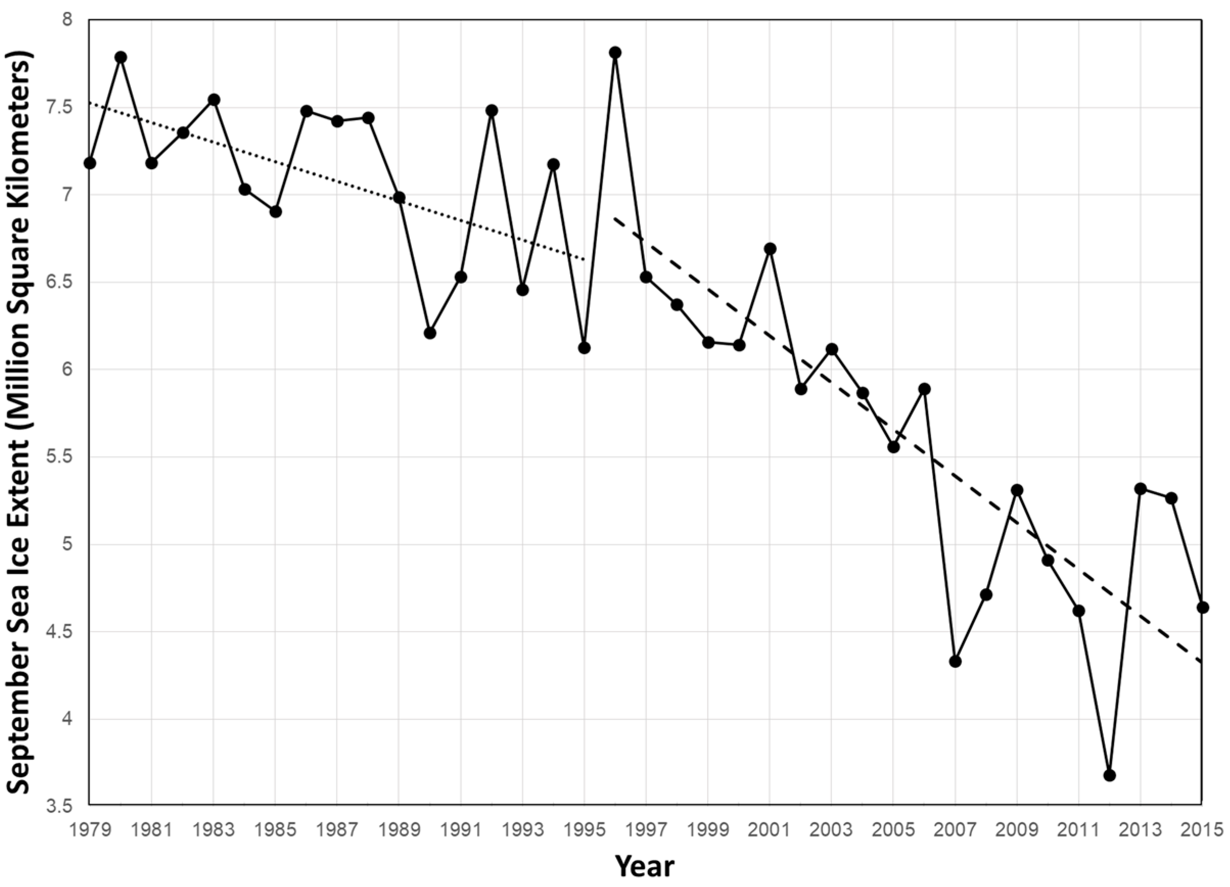
Global warming and climate change are terms that refer to increases in global temperatures primarily caused by increases in greenhouse gases such as carbon dioxide. A warming world thus leads to climate change, which can affect weather in various ways [1]. Changes in Arctic sea ice extent (SIE) are an important proxy for global warming because temperatures in the Arctic have increased at twice the rate of the rest of the world [2]. While the overall Antarctic SIE has increased slightly, SIE in the Arctic has exhibited a long-term decline [3,4]. In Figure 1 and Vihma [2], approximately half of the SIE values in September have decreased typically early in the period from 1979 to 1995. The nine lowest September SIEs have all been recorded during the past nine years, i.e., 2007–2015. The National Snow and Ice Data Center (NSIDC) reported that “Monthly September SIE for 1979 to 2015 shows a decline of 13.4% per decade relative to the 1981–2010 average” [5]. Predicting both sea ice concentrations (SICs) and SIEs is important for understanding the impacts of climate change, and developing ship navigation techniques and new Arctic shipping routes.
Information on sea ice can be obtained using: (1) remote sensing-based acquisition methods (e.g., airborne or spaceborne sensors); and (2) in situ sources, such as visual observations by citizen scientists. Passive microwave satellite data collection has been widely used because of its extended coverage and temporal resolution, despite its low spatial resolution [6,7]. Satellite data is often processed using sea ice retrieval algorithms to determine the values of various sea ice parameters, such as age, concentration, extent, thickness, and others [8]. Most sea ice data products are publicly available online.
Many approaches based on statistical or numerical models have been proposed in efforts to predict sea ice properties. Statistical models for the prediction of Arctic sea ice are constructed from historical observations and relationships among atmospheric conditions (e.g., temperature, sea level pressure, and cloud), oceanic conditions (e.g., sea surface temperature), and sea ice variables (e.g., concentration, extent, ice type, and thickness) [9,10,11]. However, statistical methods cannot take into account interactions between sea ice and the atmosphere [12]. Numerical models for ice–atmosphere interaction, ice–ocean interaction, and ice–ocean–atmosphere interaction are based on physical equations governing the system dynamics and thermodynamics; they use ice, atmosphere, and ocean properties as input variables [12,13]. Numerical models typically outperform statistical models in short-term forecasting [10]. Unfortunately, although inputs such as atmosphere, ocean and ice parameters can be obtained from remote sensing data, they must be calibrated and validated with spatially and temporarily well distributed in situ observations, which is both difficult and costly.
Machine learning is a field of study in computer science and a type of artificial intelligence that provides the capability to learn or to predict data using computational methods. Machine learning has been used extensively in diverse applications such as biology, computer vision, economics, and remote sensing [14,15]. With recent advances in hardware, techniques, optimization skills, and data collection, deep learning (DL), which is rooted in artificial neural network theory, has recently become a major area of focus in the machine learning community because of its potential for better learning representations of data using multiple layers instead of a shallow architecture [16]. In the 2000s, solutions were derived to the problems of overfitting and high computational demand that are typical of neural networks, permitting much larger and much deeper neural networks to be developed. DL has become a fast-growing subfield of machine learning. In the geosciences, the acquisition of large volumes of remote sensing data is accelerating because of the proliferation of sensing techniques and sources. These large volumes or quantities of data are often referred to as “big data”. For example, massive daily SIC images are the representative of big data that can be obtained in the Polar Regions. In the Arctic, more than 13,000 daily SIC images have been acquired since 1978 and images will continue to be collected. Furthermore, historical datasets contain seasonal SIC signals numbering in the tens of millions. Analysis of big data consisting of remote sensing images poses a problem in that it may be impossible to find an optimal balance between discriminability and robustness. DL techniques have proven to be effective in addressing this situation. In remote sensing fields, therefore, various studies have been undertaken using DL architectures for image pre-processing, classification, target recognition, and scene understanding [17].
In this study, we use a DL framework that has received considerable attention in various industries and multidisciplinary studies. This framework involves the use of high-temporal-frequency remote sensing images to forecast monthly Arctic SICs. Unlike traditional numerical or statistical models that couple atmospheric, ice, and ocean states to predict sea ice, the DL framework employed in this study uses only monthly SIC data acquired by passive microwave sensors as input data to a DL-based fitting model. While obtaining data on the physical parameters of the atmosphere, sea ice, and the ocean is costly, remote sensing data are easy to obtain over extended areas and to archive historically. In this study, we address: (1) the reconstruction of future SIC images using the proposed DL-based methods, and (2) a quantitative and qualitative comparisons of the new technique with existing methods. This paper is organized as follows. In the materials and methods section, we discuss time series forecasting, the DL framework used in this study, including hyperparameter tuning for the most appropriate DL models, as well as data description. In the results and discussions sections, the experiments that were conducted using the proposed framework and the results obtained are presented and discussed. The conclusions section summarizes the contributions of this study and outlines possible directions for future research.
2. Materials and Methods
2.1. Time Series Forecasting as Supervised Learning
“A time series is a sequence of observations taken sequentially in time [18]”. A time series is characterized by an explicit order between observations that is referred to as the “time dimension”. There are two goals in exploiting time series: (1) understanding or describing a dataset, which is referred to as “time series analysis”, and (2) making predictions, which is referred to as “time series forecasting”. While time series analysis improves the understanding of the underlying problems in observations by identifying seasonal patterns, trends, external factors, and other characteristics of the observations, time series forecasting makes predictions about the future using models that are fitted to historical data [18,19]. The SIC data used in this study is also time series data. SIC data have been generated daily since 1978 from data collected by passive microwave sensors and will be generated continuously in the future. The SIC data collected daily at each geographical location reveal seasonal patterns and trends in the sea ice dynamics of the Arctic and Antarctic oceans.
Supervised learning, which has been widely used in practical machine learning applications, employs an algorithm to map input variables to outputs by developing learning functions. Supervised learning consists of two components and can be framed as a time series problem: (1) training the data using known inputs and outputs for the best fitted model, which is equivalent to “time series analysis”, and (2) predicting output variables for unknown observations, which is equivalent to “time series forecasting”. For example, Table 1 lists sample values for monthly Arctic SIC data collected from April to December. Given the SIC value for the current month , we predict the SIC value for the next month by phrasing a time series forecasting problem as a regression problem when the output variable is a real value rather than a categorical value. As Table 2 shows, we can develop a simple supervised learning function , which is either a linear or nonlinear function , to map input data to output (predicted) data . If is a linear function with one input variable, for example, it can be expressed as , where is the SIC value at time , and are coefficients found by minimizing fitting errors of . This prediction problem can also be phased using multiple time steps as shown in Table 3. For instance, if we have three input variables, the current month as well as two prior time steps and , the learning function can be written as . In this way, time series problems can be explained in a supervised manner, but finding the optimal coefficients while satisfying all training data is complicated and difficult.
2.2. Deep Learning
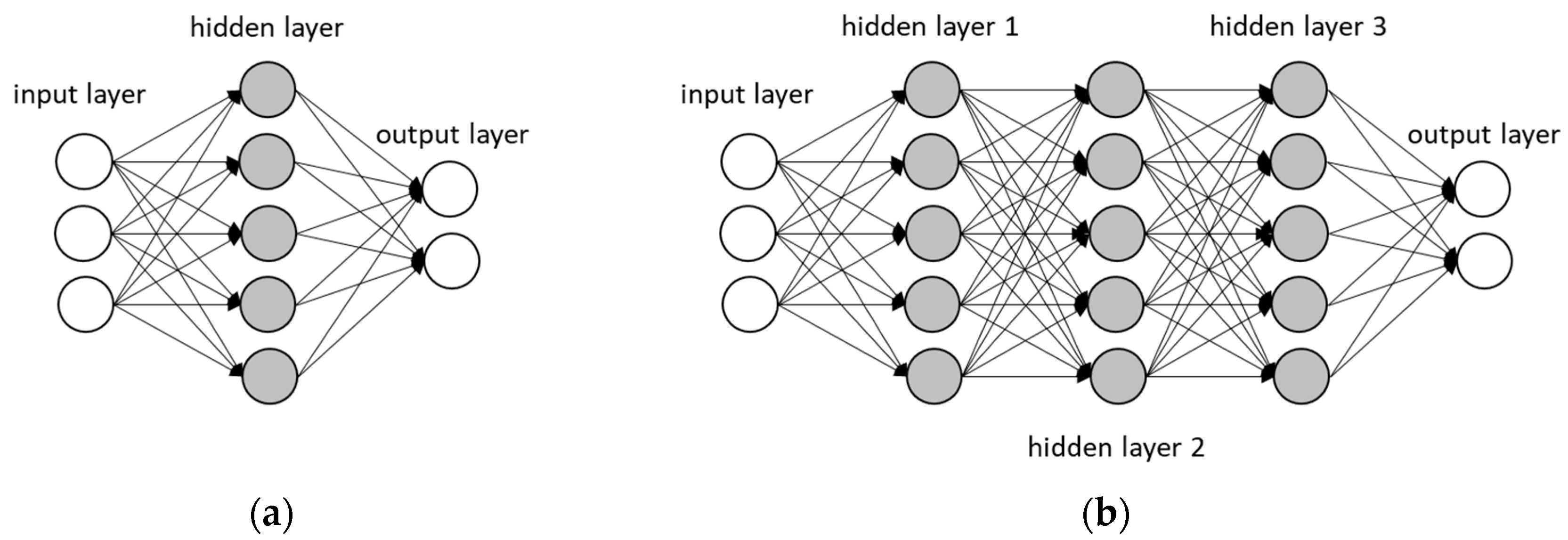
Deep learning is a relatively new subfield of machine learning that was inspired by artificial neural networks that were developed in the late 1980s. The development of faster computers and the growing availability of large datasets to train large neural networks, accompanied by increased investment in the technology, has resulted in an exponential growth into DL research [16,17,20]. As Figure 2 shows, perceptrons or neurons (the grey circles in Figure 2) in hidden layers, which are simple computational units, inter-connect weighted input (or visible) layers to output layers using an activation function [16,17]. The primary difference between deep neural networks and traditional neural networks is that deep neural networks (Figure 2b) have more than two hidden layers in the network, while the latter (Figure 2a) have only one hidden layer. In a deep network architecture, neurons in the first hidden layer make simple decisions, such as the weighting of the input variables, and neurons in the second hidden layer then make more complex and more abstract decisions than the neurons in the first hidden layer [16]. In this way, a network with multiple hidden layers can technically engage in more complicated decision making.
In this study, we used two deep learning approaches: (1) a multilayer perceptron (MLP) and (2) a long and short-term memory (LSTM) to predict monthly Arctic SIC values in a supervised manner.
An MLP, also known as a “feedforward neural network”, is the most useful type of neural network. In an MLP, the outputs predicted by training the network with given inputs may not be equal to the desired values. Since there may be errors between the actual and desired outputs, the training algorithm uses the errors to iteratively adjust the weights in the network. Therefore, the network can eventually obtain the optimal results via an iterative process. The steps involved in implementation of an MLP can be described as follows [21]:
- Initialize network weights.
- Pass the weighted inputs through an activation function.
- Calculate an error between the output of the network and the expected output.
- Propagate the error in Step 3 back through the network.
- Update the weights to minimize the overall error.
- Repeat Steps 2–5 until the error is smaller than a user-specified threshold or until the maximum number of iterations (epochs) is reached.
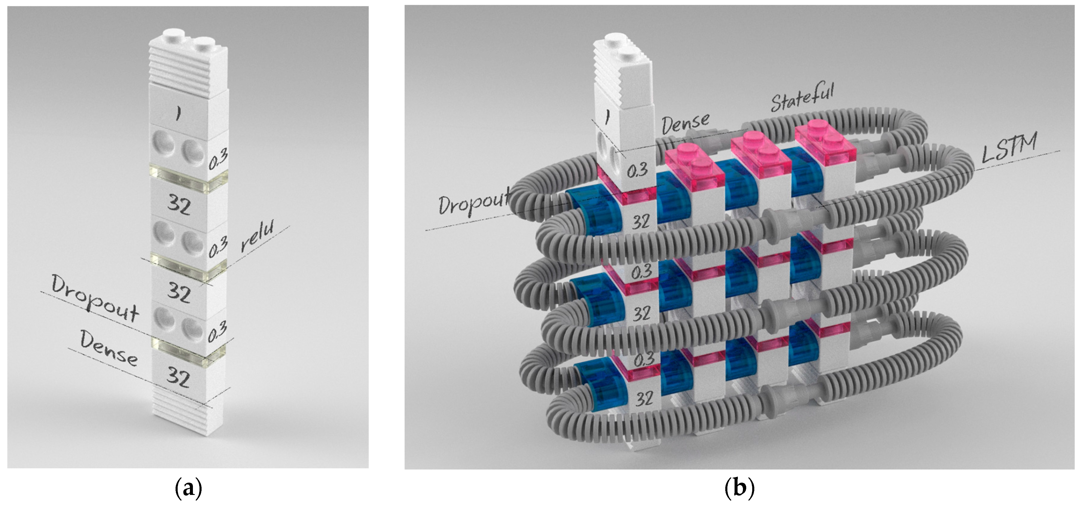
Although an MLP can be applied to sequence prediction problems, there are some limitations of having to specify the scope of temporal dependence between observations. The LSTM is a type of recurrent neural network, which is a special type of neural network designed for sequence problems, and has promise for the analysis of time series data. The LSTM contains loops that feed the network states from a previous time step as inputs to the network to influence predictions at the current time step. Since each unit of the LSTM consists of cells with gates that contain input/forget/output information, it can hold long-term temporal sequence better than a standard feedforward MLP network [22]. The basic steps of the LSTM are similar to the MLP, but as shown in Figure 3, the LSTM has an additional recurrent process (i.e., blue blocks and grey pipelines in Figure 3b) to deliver learning status to the next learning step. Although the LSTM generally outperforms the MLP for long-term sequence predictions, the high computational overhead is problematic.
The configuration of the parameters used in DL models is critical to obtaining good performance [23]. Neural networks require many parameters whose values need to be set before models are developed, and they are quite difficult to optimize. There are preferred configurations in practice for choosing some algorithms and options. For example, small random numbers for weight initialization, a rectifier activation function, and an Adam (Adaptive Moment Estimation) gradient descent optimization algorithm with a logarithmic loss function typically perform well in practice [24]. However, in iterative gradient descent, the batch size (the number of patterns shown to the network before updating of the weights), the number of epochs (the number of iterations of showing the entire training data set to the network during training), and the numbers of layers and neurons (or memory cells) used to determine network topology should be tuned for each dataset, because they depend greatly on which dataset is used [25]. To find the optimal combination of parameter values that maximize model scores, all combinations of parameters should be tested using a grid search, which is the traditional and common approach to performing parameter optimization [26]. Since grid searching may be notoriously time-consuming, parallel processing is used to identify the best parameter value combinations.
Once both DL models have been trained, they can be used to test or validate the model using a dataset other than the original training set, prior to the MLP being used in practice. This will provide a statistical measure of the performance of the model and an estimate of its performance on unseen data. The network topology can then be used to continuously and operationally make predictions of future output values.
2.3. Data Description and Preprocessing
Since 1978, multiple spaceborne remote sensing instruments (e.g., the Scanning Multi-channel Microwave Radio-meter (SMMR) on the Nimbus 7 satellite, Special Sensor Microwave/Imagers (SSM/Is) on the Defense Meteorological Satellite Program (DMSP)-F8, -F11, and -F13 satellites, and the Special Sensor Microwave Imager/Sounder (SSMIS) on the DMSP-F17 satellites) have collected daily images. These have been used to generate SIC images by applying the NASA (National Aeronautics and Space Administration) Team algorithm [6]. Due to long-term observations from different sensors, several techniques (e.g., mapping data onto a common grid, addressing instrument drift, adjusting land-to-ocean spill over, replacement of bad data) are employed to solve or reduce inter-sensor corrections [6]. The NSIDC provides gridded SIC data at a 25-km spatial resolution in the polar stereographic projection.
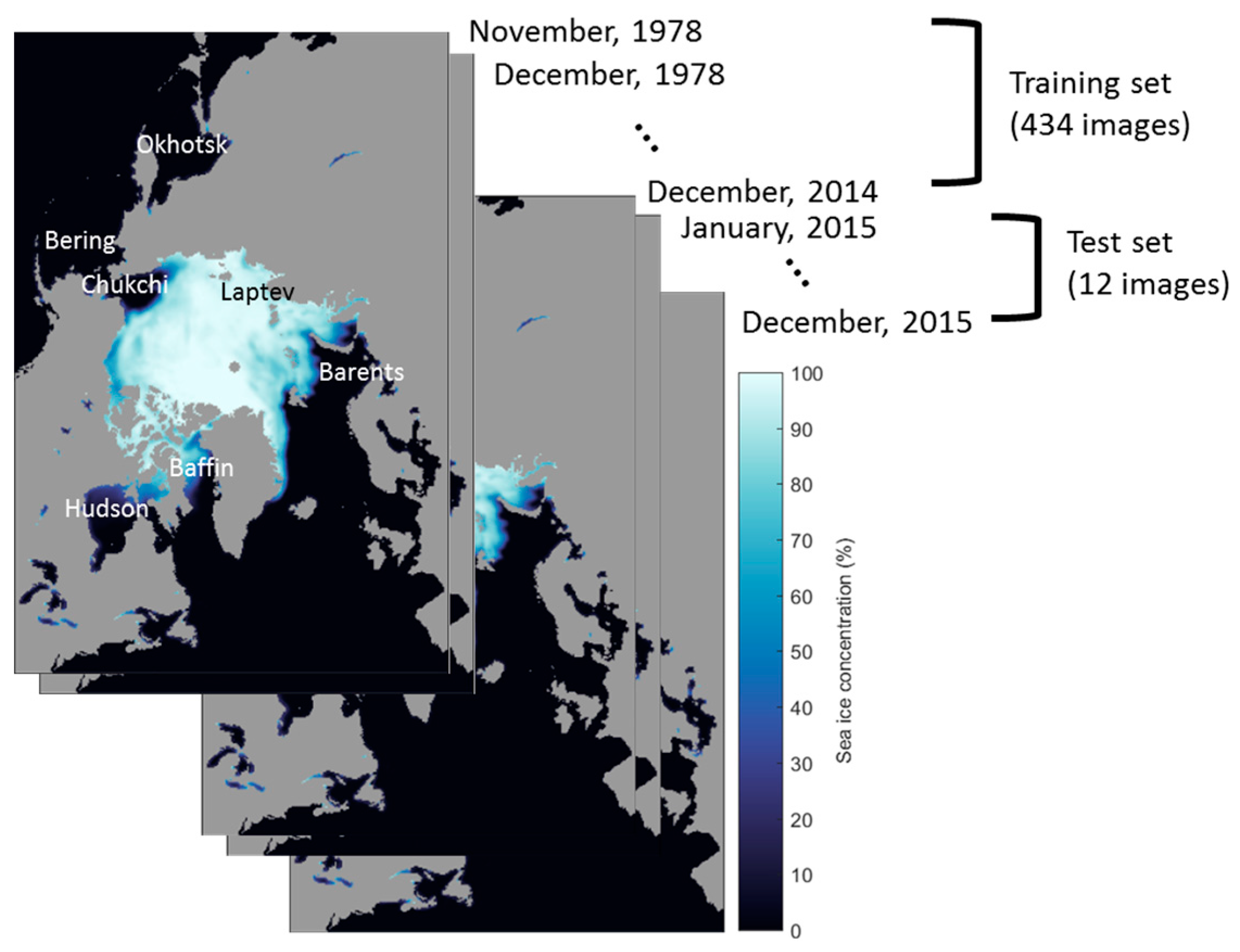
In this study, we used monthly Arctic SIC data that was generated from daily data provided by the NSIDC (available at www.nsidc.org). Because of instrument errors, low spatial resolution, and sea ice movements in daily images, near-real-time (daily) data is limited for operational use, although it is useful for monitoring subtle changes in sea ice coverage or day-to-day shipping operations. Simple averaging over an entire month helps to reduce some day-to-day noise inherent in daily sea ice measurements. In this study, a total of 446 months of monthly Arctic SIC data, acquired from November 1978 to December 2015, was used. The data acquired from November 1978 to December 2014 was used as the training dataset, and the data acquired from January 2015 to December 2015 was used as the test dataset, as illustrated in Figure 4. Despite the use of monthly data instead of daily data, there are still more than 28 million monthly sequential time series. For example, if we used 12 previous observations, there are 422 sequential time series at each pixel location from the training images. Since the number of effective pixels in an image is 67,884 (i.e., we excluded land areas), there are 28,647,048 time series. However, some regions have identical time series, such as the open sea areas, so we removed these redundancies, leaving roughly 12 million unique data. This is sufficient to apply the DL architecture for model training.
3. Results
3.1. Predictions and Comparisons of Monthly Sea Ice Concentration
A measure of the performance of a time series model is its ability to produce good forecasts. This ability is often tested using split-sample experiments, in which the model is fitted to the first part of a known data sequence and forecasts are obtained for the latter part of the series. The predicted values are then compared with the known observations. The goal is to minimize the foresting errors so that the predicted future values are as close as possible to actual future values.
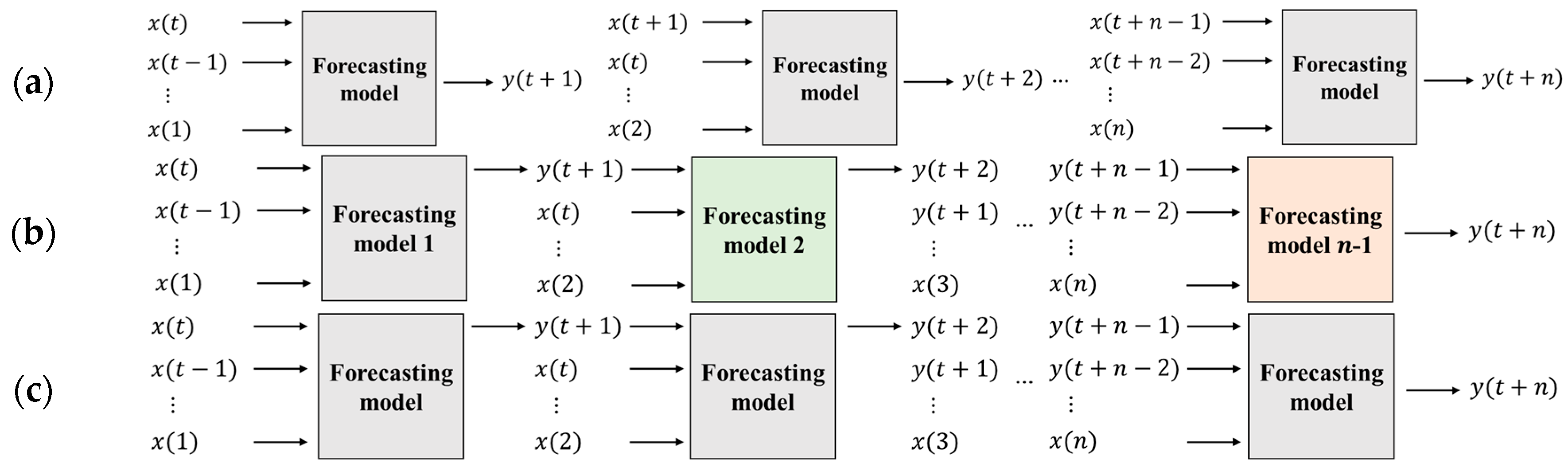
Time series forecasting is normally made only one-step prediction based on past observations, as shown in Table 3 and Figure 5a. To solve problems of multiple-step ahead prediction, two approaches are often considered: (1) a direct model re-training approach and (2) a recursive approach [29]. The re-training strategy re-trains the forecasting model when new predictions are made as shown in Figure 5b. In the case of predicting SIC for the next two months, for example, we would develop a model for the first month and a separate model for the second month. This approach may develop more fitted models and may produce unexpected results, but its extremely high computational overhead is problematic in practice, especially for training our massive sea ice data. The recursive approach uses a single prediction model multiple times. The predicted value for time step is used as an input for making a prediction at the following time step , as shown in Figure 5c. The recursive approach is not computationally intensive, because it does not require a re-training process when new predictions are entered. However, prediction errors may quickly increase and may be accumulated, because the prediction at is dependent on the prediction at .
Monthly forecasts for 2015 were made by fitting a model to the first 434 months of the time series and using this model to predict monthly SIC values for the last 12 months of the time series in two ways: (1) one-month (short-term) prediction and (2) one-year (long-term) prediction using a recursive approach. In one-month prediction, the sensitivity of the prediction model according to month can be obtained, but it can only predict one time step into the future. For long-term prediction, sequentially predicted SIC values are used as input values of the pre-trained single DL model.
3.1.1. Short-Term (One-Step Ahead) Predictions of Monthly Sea Ice Concentration
As mentioned in the previous section, we used the most popular initialization, activation and optimization algorithms and tuned the batch size, the numbers of epochs, the number of hidden layers, and the number of neurons (or memory cells for the LSTM) using a parallelized grid search to configure the hyperparameters for fitting the network topologies. However, if we used the network deep enough and had enough iterations, the DL models eventually converged to a high accuracy outcome. Therefore, we chose three hidden layers with 32 neurons (or memory cells for the LSTM) each. The batch size and the number of epochs were set to 12 and 200, respectively. Then we initialized the network weights using small random values from a uniform distribution and used the rectifier, also known as rectified linear unit (ReLU) activation function, which has shown improved performance in recent studies, on each layer. Dropout layers with a rate of 0.3 were added after each hidden layer to prevent overfitting. The Adam optimization algorithm, which is efficient in practice, was chosen. Detailed network topologies for MLP and LSTM are described in Figure 3. To quantitatively and qualitatively evaluate the performance of the proposed DL-based prediction models, we used an autoregressive (AR) model, which is a simple and traditional statistics-based time series model. An AR model also uses observations from previous time steps as inputs to a regression equation to predict the value at the next time step [30,31,32]. Because an AR model can be used to solve various types of time series problems [32], it is a good baseline model for evaluating the performance of our proposed DL-based models. Both AR and DL-based models require that the number of past observations be known. Because SIC data often exhibit annual patterns, 12 previous observations were employed to develop all prediction models.
We first evaluated quantitative accuracies of the models by calculating root mean square errors (RMSEs) between the actual and predicted values as listed in Table 4. To prevent the overall RMSE decreasing because of the effect on very small error values over open sea or melted areas in summer, we used pixels that actually contained sea ice in either observed or predicted data for RMSE computations. Over the course of the year, both MLP and LSTM DL-based predictions typically exhibited better agreement with the observed values than the AR-based predictions. The monthly mean RMSE of the LSTM slightly outperformed the MLP.
RMSE values in the summer melting season, especially from July to October, were much larger than those in other seasons. As shown in Figure 6, which illustrates the 10-year moving mean (blue solid line) and variability (orange solid line) of sea ice anomalies (blue dotted line) from 1979 to 2015, winter and spring variability were small and did not significantly change from 1979 to 2015, but summer and fall variability dramatically increased in the 2000s. Therefore, it should be noted that there is a relationship between the high RMSE values of recent sea ice predictions and the high variability of sea ice anomalies in summer. The seasonal average comparisons summarized in Table 5 show that the DL models also outperformed AR model for both freezing and melting seasons. The average RMSE difference between the results of the AR and DL approaches for melting season (3.64% for MLP; 3.94% for LSTM) was relatively large compared to the difference for freezing season (2.68% for MLP; 2.99% for LSTM).
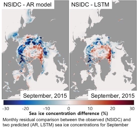
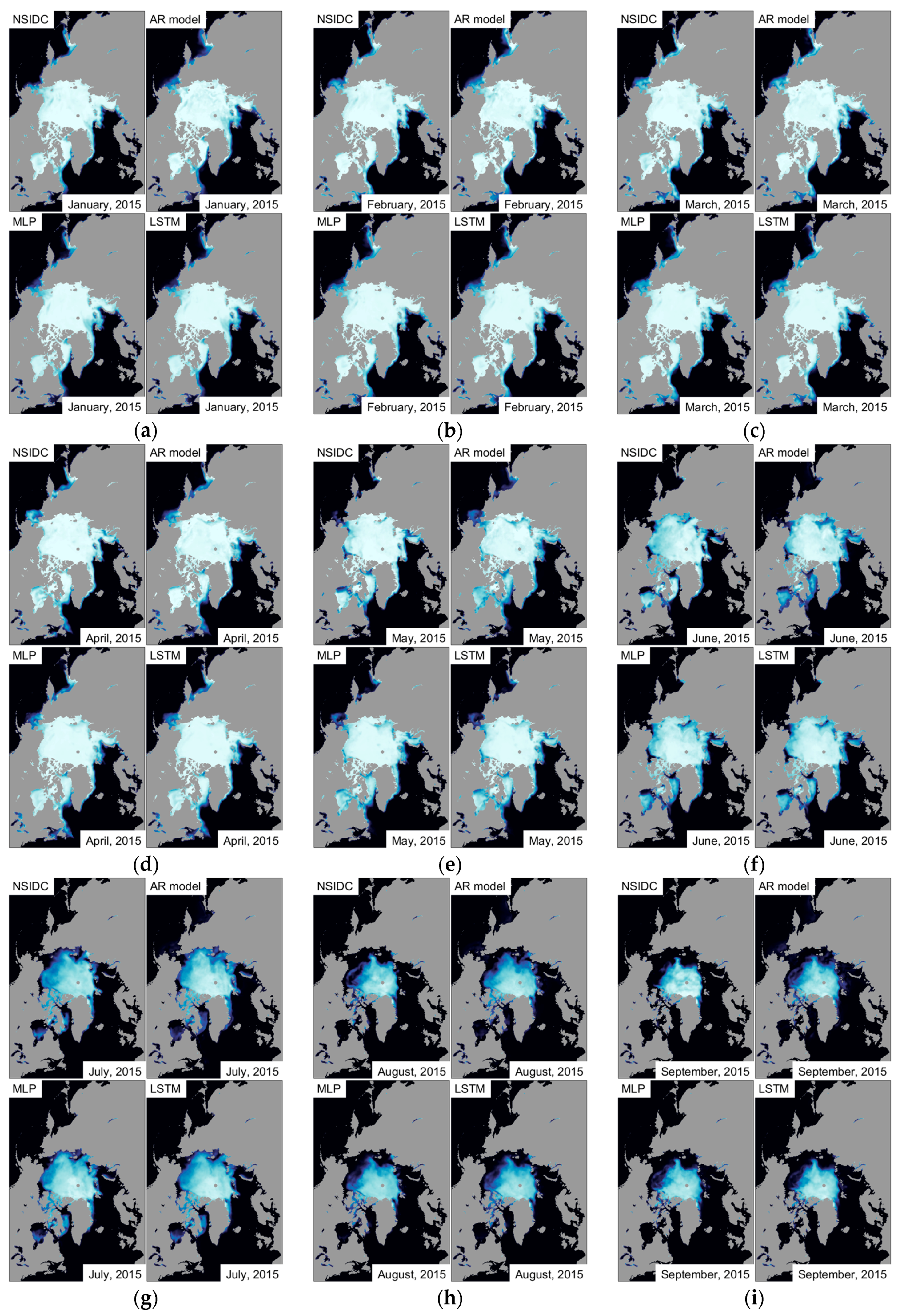
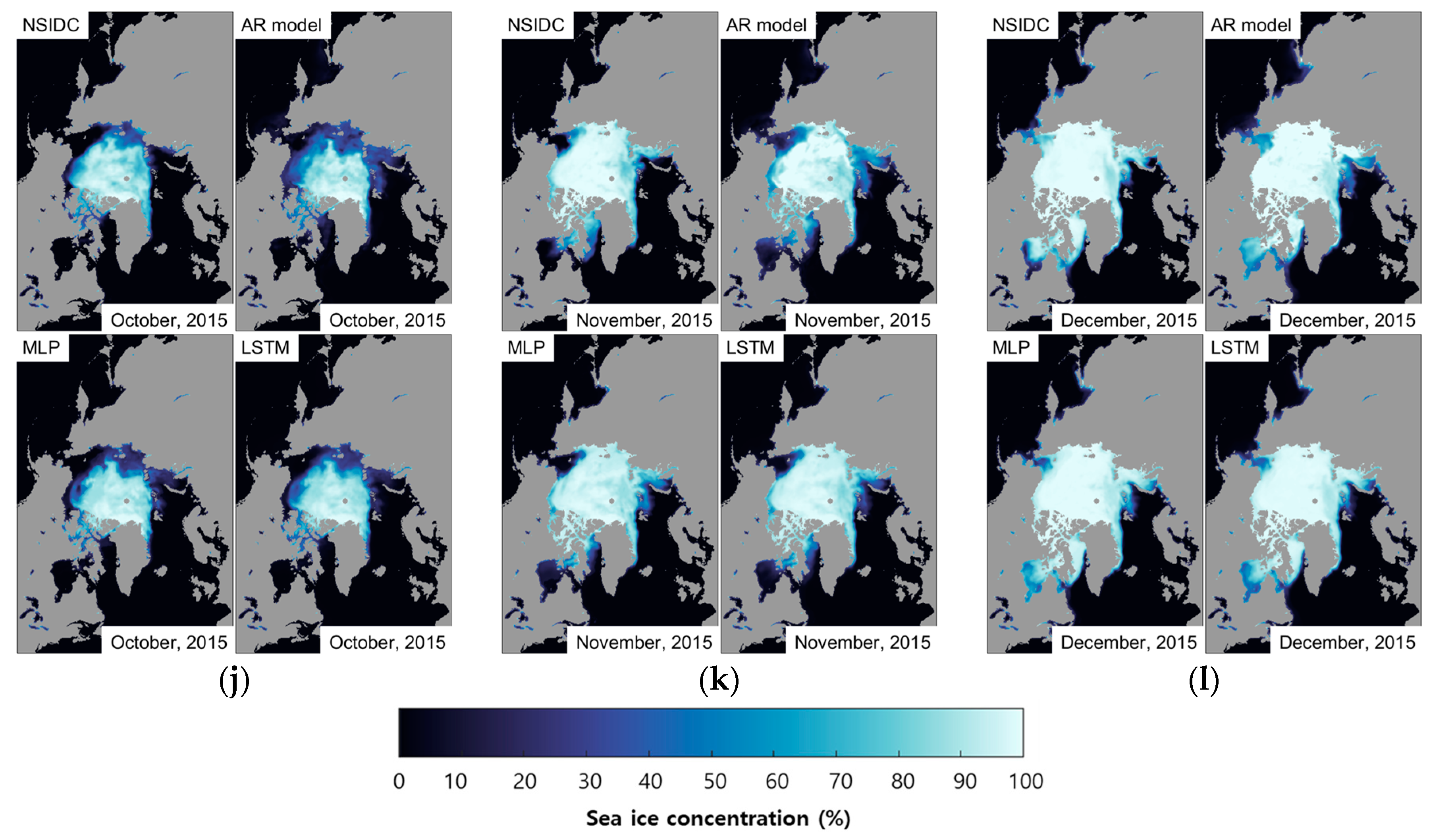
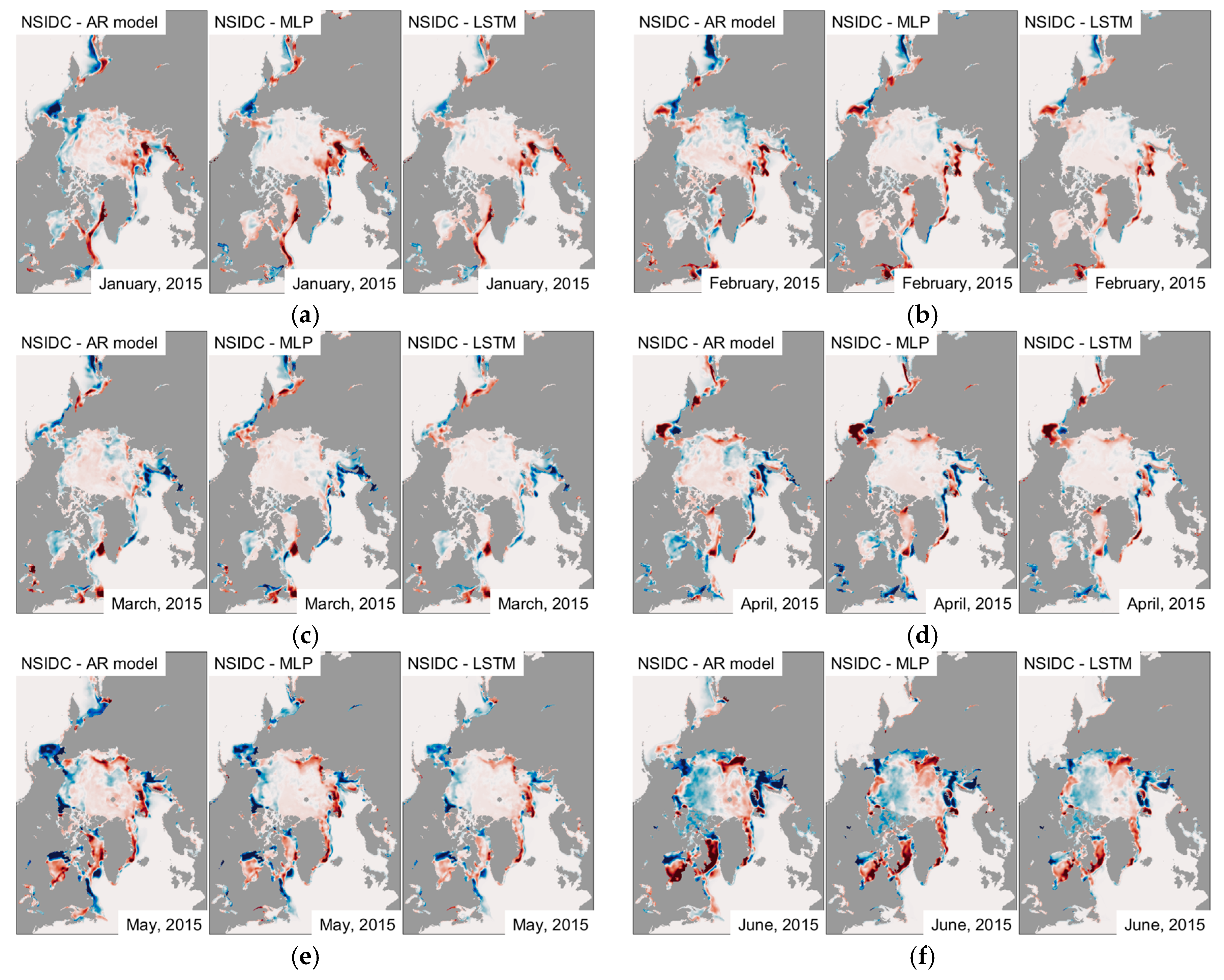
As a qualitative evaluation of the models, we performed a visual inspection of the monthly predicted SICs by comparison with the observed images, to assess how well the forecasting models predicted future SICs. Figure 7 illustrates 12-month SIC sets for 2015. Each monthly set consists of four images: (1) the observed SIC (upper left); (2) the predicted SIC obtained using the AR model (upper right); (3) the predicted SIC obtained using the MLP-DL model (lower left), and; (4) the predicted SIC obtained using the LSTM-DL model (lower right). Brighter pixels are associated with higher SIC values; the grey circle centered on the North Pole indicates where the central Arctic is invisible to the satellite instruments used to generate these images. Figure 8 shows the spatial patterns of monthly residual images, highlighting the differences between the observed and predicted values. The image on the left in each monthly set represents the AR model error, the image on the middle represents the MLP-DL model error, and the image on the right represents the LSTM-DL model error. In Figure 8, areas with predicted ice concentration greater than the observed ice concentration (overestimated areas) are indicated in blue, and areas with predicted ice concentration less than the observed ice concentration (underestimated areas) are indicated in red. Overall, as both Figure 7 and Figure 8 show, the errors in the predicted winter ice cover over the central Arctic Ocean were small. Most of the anomalies in the predicted SIC occurred in the North Atlantic and North Pacific Oceans, as a result of fluctuations in the ice edge. Greater variations occurred in the predicted summer sea ice over the central Arctic Ocean. Evaluation of the prediction model performance showed that the AR model often generated more overestimated and underestimated pixels than the DL model-based images. While both DL models generated quantitatively and qualitatively similar outputs, the SIC images predicted by the LSTM model showed slightly better agreements with the observed images than the MLP model-based images (i.e., geographical locations of overestimated and underestimated regions are similar, but the amount of the LSTM errors is slightly smaller than the MLP). A brief qualitative explanation for each month is presented below. The names of the locations are shown in Figure 4.
The January and February images show that both models yielded very accurate predictions over the central Arctic, but some discrepancies were present on the Pacific and Atlantic margins. The AR model overestimated sea ice in the Sea of Okhotsk and the Bering Sea, while sea ice in the Barents Sea was underestimated by the AR model in comparison to the DL-based models. For March, the AR model predicted more sea ice areas in both the Sea of Okhotsk and the Barents Sea than the proposed model. The April image predicted by the AR model contained more inaccurately predicted SIC values in both the Atlantic and Pacific Oceans than the DL models. From January to April, both prediction images over the central Arctic, where SIC values are high, exhibited better agreement with the observed images, whereas errors were typically observed near the ice edge. For May and June, when sea ice melting begins, much higher residuals were observed in multiple areas (e.g., the Bering Sea, the Chukchi Sea, the Laptev Sea, the Barents Sea, the Baffin Bay, and the Hudson Bay) in the AR-based prediction images than in the DL model-based images. Sea ice residuals that were often present near the ice edge in winter move to the central Arctic as melting progresses. For the summer melt season (July to September), both models predicted higher-than-observed SICs in the Arctic Ocean. The total amount of sea ice predicted for the Northern Hemisphere by the AR model was much larger than that predicted by the DL models. As mentioned in the introduction, Arctic SIE has declined, and the summer rate of decline has accelerated, in recent years. Large overestimations for the summer months were obtained with both the AR and DL models, especially in the AR-predicted images. This indicates that the AR model may not capture this unusual trend as well as the DL models. The AR predictions for October, when sea ice is freezing, exhibited large underestimations along the ice margin in the Chukchi, Laptev, and Barents Seas. The DL models yielded similar underestimates, but the underestimated areas are much smaller than those resulting from use of the AR model. Mid-September is the sea ice minima and late-September is the onset of the freezing season. In the last few years, however, late-September sea ice growth has slowed down resulting in an increased October growth rate. In October 2015, the average SIE increased by roughly 67% compared to September (i.e., 4.63 million square kilometers in September; 7.72 million square kilometers in October as reported by the NSIDC [33]). Similar to summer predictions, the prediction models, especially the AR model, could not properly capture this quick change. The DL models also could not capture the change, but they were better than the AR model. This indicates that the DL models, which can make more complicated decisions, may respond better to this rapid increase in sea ice than the AR model. Similar to other winter SIC images, for the period from November to December, the predicted images showed visually similar error patterns, but the images predicted by the AR model contained more dark blue and dark red pixels, as Figure 8 shows, indicating more significantly overestimated and underestimated sea ice areas, respectively, in the central Arctic area, in comparison to the DL model predictions.
3.1.2. Long-Term (Multi-Step Ahead) Predictions of Monthly Sea Ice Concentration
To evaluate the performance of our DL-based model for multiple-step ahead predictions, additional experiments were conducted using a recursive approach. The same single DL model that was used in the one-step ahead predictions (trained using data from 1978 to 2014) was used here; the predicted values were used as inputs multiple times for the long-term predictions (see Figure 5c). Table 6 lists the monthly prediction errors (RMSEs) of the one-year predictions with the differences from the results of one-step predictions in the previous section. For example, the RMSE values of the last column of the table indicate the December 2015 predictions, made using observations from December 2014, and prediction results from January to November 2015 as inputs (12-month lead time). For the September SIC prediction, while the RMSEs of the one-step ahead prediction using the MLP and the LSTM were 9.69 and 9.41, respectively, the RMSE values predicted eight months in advance were 17.47 and 12.44, respectively. We trained the model using data from 1978 to 2014 and predicted SIC values to make further predictions over the course of one year, which may have exacerbated errors in the long-term predictions. While both MLP and LSTM models resulted in statistically and visually similar outcomes for the short-term predictions as shown in the previous section, for the long-term prediction, the LSTM generated small and consistent prediction errors regardless of the lead time compared to the MLP predictions (i.e., 2.14–8.75% for MLP; 1.08–3.03% for LSTM).
3.2. Predictions and Comparisons of Monthly Sea Ice Extent
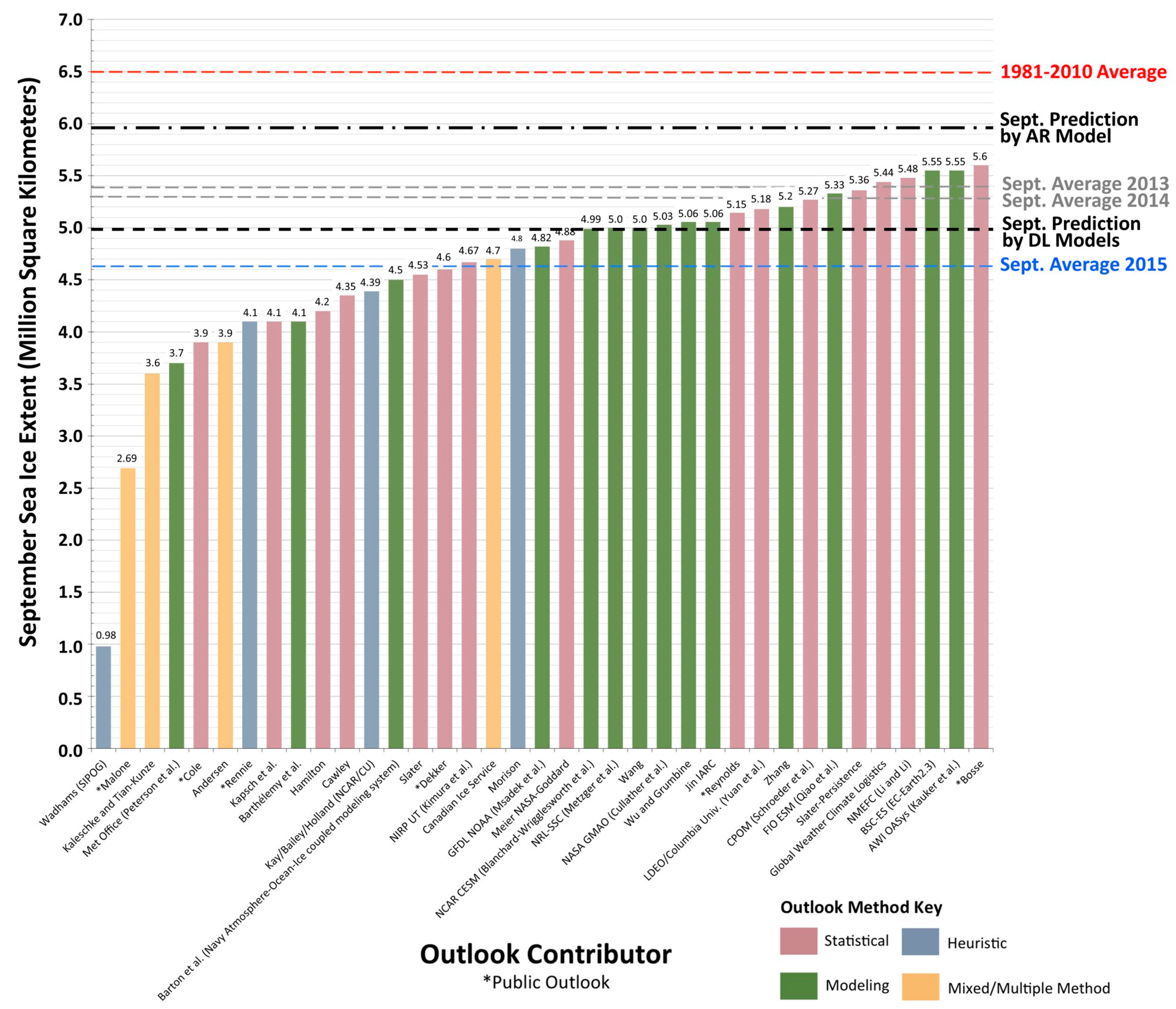
The Sea Ice Outlook (SIO) is an open process that has been available since 2008 for those interested in Arctic sea ice to share their predictions of the September SIE. September SIE predictions have been published in June, July, and August of each year since 2008, based on a variety of perspectives, including modelling, statistical, and heuristic approaches [11]. According to all SIO contributions, the median SIO predictions were close to the SIE observed before 2011. However, prediction errors have increased since 2012. In 2012, the observed SIE was much lower than predicted, whereas in 2013, it was much higher. These observations show that the prediction of Arctic sea ice has become more difficult as global warming has progressed.
The SIE is defined as the regions with ice concentrations exceeding a 15% threshold [34]. Monthly SIEs from SICs predicted using AR and DL approaches in Section 3.1.1 are calculated using this criterion, and we compared the observed SIEs with the predicted values. The SIE differences between the actual observations and the AR- and DL-based predictions are tabulated in Table 7. The SIE results obtained using the DL-based prediction, like the SIC results, exhibited better agreement with the passive microwave data throughout the year, although both approaches overestimated SIEs for every month. The observed increase in SIE prediction errors could be attributed to acceleration of the rate of decline of Arctic sea ice. The mean differences for the AR-, the MLP- and the LSTM-based models for the 12-month period were 7.94%, 3.12% and 2.80%, respectively. While all models predicted easy-to-forecast winter SIEs well, the summer predictions by the DL models outperformed the AR model predictions. For the most interesting September SIE prediction, the mean error of the DL predictions was 7.87%, whereas the error of the AR prediction was 28.66%. A comparison of the November and December SIEs, which may include long-term prediction noise, showed that the proposed DL model resulted in more accurate outcomes than the AR model.
To evaluate the accuracy of our results, we compared 37 SIO contributions for the September SIE predictions reported for August 2015 as shown in Figure 9. The observed September 2015 Arctic SIE was 4.63 million square kilometers (reported by the Sea Ice Prediction Network, SIPN; https://www.arcus.org/sipn). However, this number varies slightly depending on the processing algorithm. We calculated 4.64 million square kilometers, which is the fourth lowest record since 1979. The September SIEs submitted by the 37 SIO contributors were predicted using statistical, dynamic, and heuristic methods. The median September estimate, based on the 37 contributions, was 4.8 million square kilometers, with a quartile range of 4.2 to 5.2 million square kilometers. As Table 7 shows, our predictions using the MLP and the LSTM models were 5.02 and 4.99 million square kilometers, respectively, whereas the AR model estimate was 5.97 million square kilometers for the September 2015 Arctic SIE.
4. Discussion
In short-term (one-step ahead) predictions, both MLP and LSTM DL-based models generated statistically and visually improved prediction results compared to a traditional statistics-based model. The predictions in the freezing season were generally accurate, but during the summer months the predictions were less accurate. These results may be explained by the facts that sea ice variations during the freezing season are more stable and more predictable than in other seasons and that the AR model predicted sea ice in winter relatively well, compared to that in the melting season, although the volume of sea ice is highest in winter. We anticipate that accurate prediction of summer sea ice may be difficult because of high sea ice variability in melting zones and unexpectedly faster summer ice melting than in the past. This is a topic of interest to many researchers. As Table 4 and Table 5 show, high RMSE values were obtained with both approaches for summer, which supports this premise. Additionally, as Figure 7 and Figure 8 show, the visual inspection results obtained are similar to the statistical results; errors increased as the melting progressed and the DL methods outperformed the AR model. As mentioned in the results section, large overestimations and underestimations near the marginal ice zones occurred in both approaches at the onsets of the melting and freezing, respectively. A possible explanation for this overestimation and underestimation might be that all statistical prediction models may have a weakness for predicting dramatic or unusual changes in the volume of sea ice since sea ice decline has accelerated and growth has slowed down in the last few years. In long-term (multi-step ahead) predictions, the LSTM yielded smaller and more consistent prediction errors than the MLP as shown in Table 6. This should be noted that the LSTM was able to remember past states of the time series by minimizing the impact of degradation, compared to the MLP.
Finally, we obtained a reasonable prediction result for the September SIE by comparing the 37 predicted September SIEs submitted to SIPN. The proposed prediction models slightly overestimated the September SIE in comparison to the median of the SIO contributions. Considering the difficulty associated with accurately predicting the September SIE because of the rapid melting rate, our estimate within the quartile range of 4.2 to 5.2 million square kilometers (see Figure 9) can be considered reasonable. There are several possible explanations for this result. First, our monthly SIEs were generated using monthly data, whereas the reference data produced by NSIDC and the data of most of the contributors were calculated on a daily basis. Second and more importantly, SIO contributions reflect many other factors, such as physical parameters and subjective information, whereas only monthly passive microwave data were used as inputs for the proposed prediction method. We also developed a prediction model using SIC datasets collected until 2014. Other contributors may or may not use data from January to August in developing their prediction models, but these predictions have typically been reported mostly in August. Thus, their models could reflect more recent environmental conditions in the Arctic. Considering all these factors, our SIE estimate using the DL model produced reasonable results compared to other models.
All experiments were conducted on an Intel Xeon E5-2699 (2.20 GHz, 22 cores) with a NVIDIA Titan X (3584 CUDA cores). The high computational demand, which is a major limitation of neural network models, can now be more easily handled with such advanced machines. However, this approach still requires a high computational overhead compared to the AR model, which is based on a linear combination problem. As a result, while the AR model required roughly 1.5 h, as expected, deep learning models spent much more time on training. The MLP and LSTM required roughly 7 h and 38 h, respectively. Although DL, especially LSTM is much slower than the AR model as well as the MLP, it developed better predictive models. Additionally, since it is not necessary to re-train the prediction model every day, these limitations are somewhat alleviated, and it is certainly worthwhile to develop these predictive DL techniques.
5. Conclusions
The purpose of the present study was to use a deep neural network to predict Arctic SIC, an actively researched method in the machine learning community. Unlike traditional models that exploit various environmental or physical datasets, this study used only observed sea ice data by remote sensing sensors as an input. The study results show that DL-based prediction models can be employed successfully to fit long-term Arctic SIC datasets and to forecast monthly SICs throughout a year, although the prediction quality deteriorated slightly as recent summer month sea ice melting rates have accelerated.
This study makes several noteworthy contributions to Arctic sea ice prediction by combining historical data with a state-of-the-art technique. Our proposed method statistically and visually outperformed a traditional AR model, especially for the summer months, for which errors in sea ice images predicted by the DL models were significantly lower than those predicted by the AR model. We could not directly reproduce predictions based on many other approaches, such as statistical and numerical models that rely on numerous external factors for predictions. We were, however, able to compare our prediction results, obtained using only remote sensing image data, with the September SIO reports published by SIPN, and we obtained comparable results. Both SIC and SIE were overestimated, because of the recent unexpected decline in Arctic sea ice. Although a fully image-data-driven approach that does not incorporate physical parameters may not properly capture this unusual trend as well as other approaches, the results of this study offer some insights into the prediction of Arctic sea ice.
Further research should be carried out in several topics related to this research. (1) Although we assumed that the SIC data provided by NSIDC has a guaranteed data quality, it does contain uncertainties. Calibration with higher resolution datasets such as MODIS (Moderate Resolution Imaging Spectroradiometer) or use of other sensors such as the advanced microwave scanning radiometers (AMSRs) with various retrieval algorithms will provide improved predictive models. (2) The LSTM delivered on the promise of providing robust long-term predictions, but it is computational intensive. More intelligent approaches to remove and optimize redundant inputs would be worthwhile for future work. (3) Adding environmental or physical parameters to our model, or using our results as baseline data for other approaches, would be a fruitful area for further research. Finally, inclusion of our prediction results in the SIPN as a novel approach would be worthwhile.
Acknowledgments
This study was supported by the Korea Polar Research Institute (KOPRI) grant PE17120 (Research on analytical technique for satellite observation of arctic sea ice). The authors would like to thank Taeyoung Kim (InSpace Co., Ltd., Daejeon, Korea), who provided the graphics of Figure 3.
Author Contributions
Junhwa Chi conceived, designed and performed the experiments, analyzed the results, and wrote the paper. Hyun-Cheol Kim contributed to research design, and provided analysis tools and materials.
Conflicts of Interest
The authors declare no conflict of interest.
References
- Najafi, M.R.; Zwiers, F.W.; Gillett, N.P. Attribution of Arctic temperature change to greenhouse-gas and aerosol influences. Nat. Clim. Chang. 2015, 5, 246–249. [Google Scholar] [CrossRef]
- Vihma, T. Effects of Arctic Sea Ice Decline on Weather and Climate: A Review. Surv. Geophys. 2014, 35, 1175–1214. [Google Scholar] [CrossRef]
- Stroeve, J.; Holland, M.M.; Meier, W.; Scambos, T.; Serreze, M. Arctic sea ice decline: Faster than forecast. Geophys. Res. Lett. 2007, 34. [Google Scholar] [CrossRef]
- Parkinson, C.L.; Cavalieri, D.J. Antarctic sea ice variability and trends, 1979–2010. Cryosphere 2012, 8, 871–880. [Google Scholar] [CrossRef]
- Steele, M.; Dickinson, S.; Zhang, J.; Lindsay, R. Seasonal ice loss in the Beaufort Sea: Toward synchrony and prediction. J. Geophys. 2015, 120, 1118–1132. [Google Scholar] [CrossRef]
- Cavalieri, D.J.; Parkinson, C.L.; Gloersen, P.; Zwally, H. Sea Ice Concentrations from Nimbus-7 SSMR and DMSP SSM/I-SSMIS Passive Microwave Data; Version 1; NASA DAAC at the National Snow and Ice Data Center: Boulder, CO, USA, 1996; Available online: http://0-dx-doi-org.brum.beds.ac.uk/10.5067/8GQ8LZQVL0VL (accessed on 4 September 2017).
- Spreen, G.; Kaleschke, L.; Heygster, G. Sea ice remote sensing using AMSR-E 89-GHz channels. J. Geophys. Res. 2008, 113. [Google Scholar] [CrossRef]
- Ivanova, N.; Johannessen, O.M.; Pedersen, L.T.; Tonboe, R.T. Retrieval of Arctic Sea Ice Parameters by Satellite Passive Microwave Sensors: A Comparison of Eleven Sea Ice Concentration Algorithms. IEEE Trans. Geosci. Remote Sens. 2014, 52, 7233–7246. [Google Scholar] [CrossRef]
- Lindsay, R.W.; Zhang, J.; Schweiger, A.J.; Steele, M.A. Seasonal predictions of ice extent in the Arctic Ocean. J. Geophys. Res. 2008, 113. [Google Scholar] [CrossRef]
- Guemas, V.; Blanchard-Wrigglesworth, E.; Chevallier, M.; Day, J.J.; Déqué, M.; Doblas-Reyes, F.J.; Fučkar, N.S.; Germe, A.; Hawkins, E.; Keeley, S.; et al. A review on Arctic sea-ice predictability and prediction on seasonal to decadal time-scales. Q. J. R. Meteorol. Soc. 2014, 142, 546–561. [Google Scholar] [CrossRef]
- Stroeve, J.; Hamilton, L.C.; Bitz, C.M.; Blanchard-Wrigglesworth, E. Predicting September sea ice: Ensemble skill of the SEARCH Sea Ice Outlook 2008–2013. Geophys. Res. Lett. 2014, 41, 2411–2418. [Google Scholar] [CrossRef]
- Wang, W.; Chen, M.; Kumar, A. Seasonal Prediction of Arctic Sea Ice Extent from a Coupled Dynamical Forecast System. Mon. Weather Rev. 2013, 141, 1375–1394. [Google Scholar] [CrossRef]
- Sigmond, M.; Fyfe, J.C.; Flato, G.M.; Kharin, V.V.; Merryfield, W.J. Seasonal forecast skill of Arctic sea ice area in a dynamical forecast system. Geophys. Res. Lett. 2013, 40, 529–534. [Google Scholar] [CrossRef]
- Mountrakis, G.; Im, J.; Ogole, C. Support vector machines in remote sensing: A review. ISPRS J. Photogramm. Remote Sens. 2011, 66, 247–259. [Google Scholar] [CrossRef]
- Pedregosa, F.; Varoquaux, G.; Gramfort, A.; Michel, V.; Thirion, B.; Grisel, O.; Blondel, M.; Prettenhofer, P.; Weiss, R.; Dubourg, V.; et al. Scikit-learn: Machine Learning in Python. J. Mach. Learn. Res. 2011, 12, 2825–2830. [Google Scholar]
- LeCun, Y.; Bengio, Y.; Hinton, G. Deep learning. Nature 2015, 521, 436–444. [Google Scholar] [CrossRef] [PubMed]
- Zhang, L.; Zhang, L.; Du, B. Deep learning for remote sensing data. IEEE Geosci. Remote Sens. Mag. 2016, 4, 22–40. [Google Scholar] [CrossRef]
- Box, G.E.; Jenkins, G.M.; Reinsel, G.C.; Ljung, G.M. Time Series Analysis: Forecasting and Control, 5th ed.; John Wiley & Sons: Hoboken, NJ, USA, 2016. [Google Scholar]
- Zhang, G.P. Time series forecasting using a hybrid ARIMA and neural network model. Neurocomputing 2003, 50, 159–175. [Google Scholar] [CrossRef]
- Schmidhuber, J. Deep learning in neural networks: An overview. Neural Netw. 2015, 61, 85–117. [Google Scholar] [CrossRef] [PubMed]
- Gardner, M.W.; Dorling, S.R. Artificial neural networks (the multilayer perceptron)—A review of applications in the atmospheric sciences. Atmos. Environ. 1998, 32, 2627–2636. [Google Scholar] [CrossRef]
- Sak, H.; Senior, A.; Beaufays, F. Long short-term memory recurrent neural network architectures for large scale acoustic modelling. In Proceedings of the Fifteenth Annual Conference of the International Speech Communication Association, Singapore, 14–18 September 2014. [Google Scholar]
- Bashiri, M.; Geranmayeh, A.F. Tuning the parameters of an artificial neural network using central composite design and genetic algorithm. Sci. Iran. 2011, 18, 1600–1608. [Google Scholar] [CrossRef]
- Kingma, D.P.; Ba, J.L. Adam: A Method for Stochastic Optimization. In Proceedings of the 3rd International Conference for Learning Representations, San Diego, CA, USA, 7–9 May 2015. [Google Scholar]
- Le, Q.V.; Ngiam, J.; Coates, A.; Lahiri, A.; Prochnow, B.; Ng, A.Y. On Optimization Methods for Deep Learning. In Proceedings of the 28th International Conference on Machine Learning, Bellevue, WA, USA, 28 June–2 July 2011. [Google Scholar]
- Bergstra, J.; Bengio, Y. Random Search for Hyper-Parameter Optimization. J. Mach. Learn. Res. 2012, 13, 281–305. [Google Scholar]
- Comiso, J.C.; Cavalieri, D.J.; Parkinson, C.L.; Gloersen, P. Passive microwave algorithms for sea ice concentration: A comparison of two techniques. Remote Sens. Environ. 1997, 60, 357–384. [Google Scholar] [CrossRef]
- Markus, T.; Cavalieri, D.J. An Enhancement of the NASA Team Sea Ice Algorithm. IEEE Trans. Geosci. Remote Sens. 2000, 38, 1387–1398. [Google Scholar] [CrossRef]
- Bontempi, G.; Taieb, S.B.; Borgne, Y.L. Machine learning strategies for time series forecasting. In Business Intelligence; Springer: Berlin/Heidelberg, Germany, 2013; pp. 62–77. [Google Scholar]
- Hipel, K.W.; McLeod, A.I. Time Series Modelling of Water Resources and Environmental Systems; Elsevier: Amsterdam, The Netherlands, 1994. [Google Scholar]
- Piwowar, J.M.; Ledrew, E.F. ARMA time series modelling of remote sensing imagery: A new approach for climate change studies. Int. J. Remote Sens. 2010, 23, 5225–5248. [Google Scholar] [CrossRef]
- Lesage, P.; Glangeaud, F.; Mars, J. Applications of autoregressive models and time–frequency analysis to the study of volcanic tremor and long-period events. J. Volcanol. Geotherm. Res. 2002, 114, 391–417. [Google Scholar] [CrossRef]
- Arctic Sea Ice News and Analysis. Available online: http://nsidc.org/arcticseaicenews (accessed on 15 November 2017).
- Vinnikov, K.Y.; Robock, A.; Stouffer, R.J.; Walsh, J.E.; Parkinson, C.L.; Cavalieri, D.J.; Mitchell, J.; Garrett, D.; Zakharov, V.F. Global warming and Northern Hemisphere sea ice extent. Science 1999, 286, 1934–1937. [Google Scholar] [CrossRef] [PubMed]
Figure 1.
September Arctic sea ice extent (SIE) change from 1979 to 2015.

Figure 2.
Network topology difference between (a) a traditional neural network and (b) a deep neural network.
Figure 2.
Network topology difference between (a) a traditional neural network and (b) a deep neural network.

Figure 3.
Network topology difference between (a) a multilayer perceptron (MLP) and (b) the long and short-term memory (LSTM) (e.g., four layers: three hidden layers with 32 neurons (or memory cells), one output).
Figure 3.
Network topology difference between (a) a multilayer perceptron (MLP) and (b) the long and short-term memory (LSTM) (e.g., four layers: three hidden layers with 32 neurons (or memory cells), one output).

Figure 4.
Description of SIC datasets for model training and forecasting.

Figure 5.
Architectures of forecasting approaches: (a) one-step ahead prediction, and (b) direct model re-training approach and (c) recursive approach for multi-step ahead prediction.
Figure 5.
Architectures of forecasting approaches: (a) one-step ahead prediction, and (b) direct model re-training approach and (c) recursive approach for multi-step ahead prediction.

Figure 6.
The 10-year moving mean (blue solid line) and variability (orange solid line) of sea ice anomalies (SIAs; blue dotted line) from 1979 to 2015.
Figure 6.
The 10-year moving mean (blue solid line) and variability (orange solid line) of sea ice anomalies (SIAs; blue dotted line) from 1979 to 2015.

Figure 7.
Monthly comparisons between the actual and three predicted SICs: (a) January; (b) February; (c) March; (d) April; (e) May; (f) June; (g) July; (h) August; (i) September; (j) October; (k) November; (l) December.
Figure 7.
Monthly comparisons between the actual and three predicted SICs: (a) January; (b) February; (c) March; (d) April; (e) May; (f) June; (g) July; (h) August; (i) September; (j) October; (k) November; (l) December.


Figure 8.
Monthly residual comparisons between the actual and three predicted SICs: (a) January; (b) February; (c) March; (d) April; (e) May; (f) June; (g) July; (h) August; (i) September; (j) October; (k) November; (l) December.
Figure 8.
Monthly residual comparisons between the actual and three predicted SICs: (a) January; (b) February; (c) March; (d) April; (e) May; (f) June; (g) July; (h) August; (i) September; (j) October; (k) November; (l) December.


Figure 9.
Distribution of Arctic Outlook values (August report) for September 2015 extent. (This figure is adapted from the Sea Ice Prediction Network (SIPN) and modified by adding our results.).
Figure 9.
Distribution of Arctic Outlook values (August report) for September 2015 extent. (This figure is adapted from the Sea Ice Prediction Network (SIPN) and modified by adding our results.).


Table 1.
Samples of monthly sea ice concentration (SIC) values.
| Time | April | May | June | July | August | September | October | November | December |
|---|---|---|---|---|---|---|---|---|---|
| SIC(%) | 95 | 93 | 83 | 43 | 21 | 0 | 48 | 91 | 99 |
Table 2.
Input and output values of a simple supervised learning function using one prior time step.
Table 2.
Input and output values of a simple supervised learning function using one prior time step.
| Training | Test | ||||||||
|---|---|---|---|---|---|---|---|---|---|
| 95 | 93 | 83 | 43 | 21 | 0 | 48 | 91 | 99 | |
| 93 | 83 | 43 | 21 | 0 | 48 | 91 | 99 | ? | |
Table 3.
Input and output values of supervised learning function using three prior time steps.
| Training | Test | ||||||
|---|---|---|---|---|---|---|---|
| 95 | 93 | 83 | 43 | 21 | 0 | 48 | |
| 93 | 83 | 43 | 21 | 0 | 48 | 91 | |
| 83 | 43 | 21 | 0 | 48 | 91 | 99 | |
| 43 | 21 | 0 | 48 | 91 | 99 | ? | |
Table 4.
Comparison of monthly root mean square errors (RMSE) values for the short-term predictions.
Table 4.
Comparison of monthly root mean square errors (RMSE) values for the short-term predictions.
| Model | January | February | March | April | May | June | July | August | September | October | November | December |
|---|---|---|---|---|---|---|---|---|---|---|---|---|
| AR | 8.95 | 8.66 | 8.95 | 9.67 | 12.39 | 15.82 | 15.77 | 16.97 | 11.78 | 15.16 | 12.50 | 11.58 |
| MLP | 6.45 | 6.16 | 6.82 | 6.21 | 8.97 | 11.89 | 12.74 | 10.80 | 9.69 | 11.98 | 7.69 | 10.89 |
| LSTM | 6.35 | 6.09 | 6.61 | 6.28 | 8.54 | 11.63 | 12.79 | 10.52 | 9.41 | 11.35 | 7.78 | 9.28 |
Table 5.
Comparison of seasonal and annual RMSE values for autoregressive (AR) and deep learning (DL) models.
Table 5.
Comparison of seasonal and annual RMSE values for autoregressive (AR) and deep learning (DL) models.
| Model | Freezing Season Avg. (November–April) | Melting Season Avg. (May–October) | Annual Avg. (January–December) |
|---|---|---|---|
| AR | 10.05 | 14.65 | 12.35 |
| MLP | 7.37 | 11.01 | 9.19 |
| Difference (AR-MLP) | 2.68 | 3.64 | 3.16 |
| LSTM | 7.07 | 10.71 | 8.89 |
| Difference (AR-LSTM) | 2.99 | 3.94 | 3.46 |
Table 6.
Comparison of monthly RMSE values for the long-term predictions.
| Model | January | February | March | April | May | June |
| MLP | 6.45 (+0.00) | 9.14 (+2.95) | 8.98 (+2.14) | 8.94 (+2.80) | 12.75 (+3.76) | 18.05 (+5.97) |
| LSTM | 6.35 (+0.00) | 7.18 (+1.09) | 7.69 (+1.08) | 7.86 (+1.58) | 10.98 (+2.44) | 14.01 (+2.38) |
| Model | July | August | September | October | November | December |
| MLP | 18.39 (+5.67) | 19.61 (+8.75) | 17.47 (+7.79) | 15.13 (+3.23) | 11.23 (+3.45) | 14.77 (+3.77) |
| LSTM | 15.58 (+2.79) | 13.27 (+2.75) | 12.44 (+3.03) | 13.58 (+2.23) | 10.37 (+2.59) | 11.66 (+2.38) |
Table 7.
Monthly Arctic SIE comparison between the actual observations and two prediction models in 2015.
Table 7.
Monthly Arctic SIE comparison between the actual observations and two prediction models in 2015.
| Model | January | February | March | April | May | June |
| NSIDC | 14.00 | 14.94 | 14.96 | 14.31 | 12.78 | 11.01 |
| AR | 14.55 (+3.93%) | 15.26 (+2.14%) | 15.28 (+2.14%) | 14.67 (+2.52%) | 13.70 (+7.20%) | 11.94 (+8.45%) |
| MLP | 14.13 (+0.93%) | 14.96 (+0.13%) | 15.29 (+2.21%) | 14.63 (+2.24%) | 13.27 (+3.83%) | 11.33 (+2.91%) |
| LSTM | 14.11 (+0.79%) | 15.03 (+0.60%) | 15.15 (+1.27%) | 14.58 (+1.89%) | 13.25 (+3.68%) | 11.40 (+3.54%) |
| Model | July | August | September | October | November | December |
| NSIDC | 8.70 | 5.55 | 4.64 | 7.70 | 10.07 | 12.43 |
| AR | 9.68 (+11.26%) | 6.98 (+25.77%) | 5.97 (+28.66%) | 9.04 (+17.40%) | 11.24 (+11.62%) | 13.19 (+6.11%) |
| MLP | 9.13 (+4.94%) | 6.09 (+9.73%) | 5.02 (+8.19%) | 8.08 (+4.94%) | 10.57 (+4.97%) | 12.68 (+2.01%) |
| LSTM | 8.98 (+3.22%) | 6.10 (+9.91%) | 4.99 (+7.54%) | 8.10 (+5.19%) | 10.48 (+4.07%) | 12.59 (+1.54%) |
Unit: million square kilometers.
© 2017 by the authors. Licensee MDPI, Basel, Switzerland. This article is an open access article distributed under the terms and conditions of the Creative Commons Attribution (CC BY) license (http://creativecommons.org/licenses/by/4.0/).
Share and Cite
MDPI and ACS Style
Chi, J.; Kim, H.-c. Prediction of Arctic Sea Ice Concentration Using a Fully Data Driven Deep Neural Network. Remote Sens. 2017, 9, 1305. https://0-doi-org.brum.beds.ac.uk/10.3390/rs9121305
AMA Style
Chi J, Kim H-c. Prediction of Arctic Sea Ice Concentration Using a Fully Data Driven Deep Neural Network. Remote Sensing. 2017; 9(12):1305. https://0-doi-org.brum.beds.ac.uk/10.3390/rs9121305
Chicago/Turabian StyleChi, Junhwa, and Hyun-choel Kim. 2017. "Prediction of Arctic Sea Ice Concentration Using a Fully Data Driven Deep Neural Network" Remote Sensing 9, no. 12: 1305. https://0-doi-org.brum.beds.ac.uk/10.3390/rs9121305
Note that from the first issue of 2016, this journal uses article numbers instead of page numbers. See further details here.