
A Method for Improving the Pose Accuracy of a Robot Manipulator Based on Multi-Sensor Combined Measurement and Data Fusion


Abstract
: An improvement method for the pose accuracy of a robot manipulator by using a multiple-sensor combination measuring system (MCMS) is presented. It is composed of a visual sensor, an angle sensor and a series robot. The visual sensor is utilized to measure the position of the manipulator in real time, and the angle sensor is rigidly attached to the manipulator to obtain its orientation. Due to the higher accuracy of the multi-sensor, two efficient data fusion approaches, the Kalman filter (KF) and multi-sensor optimal information fusion algorithm (MOIFA), are used to fuse the position and orientation of the manipulator. The simulation and experimental results show that the pose accuracy of the robot manipulator is improved dramatically by 38%∼78% with the multi-sensor data fusion. Comparing with reported pose accuracy improvement methods, the primary advantage of this method is that it does not require the complex solution of the kinematics parameter equations, increase of the motion constraints and the complicated procedures of the traditional vision-based methods. It makes the robot processing more autonomous and accurate. To improve the reliability and accuracy of the pose measurements of MCMS, the visual sensor repeatability is experimentally studied. An optimal range of 1 × 0.8 × 1 ∼ 2 × 0.8 × 1 m in the field of view (FOV) is indicated by the experimental results.1. Introduction
Since the first demonstration by Devol et al. in 1956, robots have been widely exploited in many fields, such as spraying, painting, spot welding, sealing, parts picking and other operations [1]. A fine accuracy in terms of the robot manipulator pose is mostly required in recent applications of industrial robots. The pose accuracy is defined precisely by ISO 9283 (1998) [2] as the deviation that occurs between the required and attained poses and the variance of the attained poses in a number of repetitions [1].
Considerable research for many years has been done about the improvement of the pose accuracy of robots. The kinematics errors refer to the differences between the kinematics parameters of a robot and its nominal values because of the manufacturing and assembly tolerance. Cost restriction aside, the kinematics calibration is an effective method to improve the absolute accuracy of robots [3]. A number of research of the kinematics calibration has been presented, e.g., Denavit and Hartenberg (1957) proposed a D-Hmodel that provided the basis for the kinematics calibration. Further, Hayati (1983) presented a revised D-H model for proposing a linear model, which related the parameter errors to the end-effector positioning error of the serial robot directly. However, these methods have limitations. For example, due to both the geometric errors and non-geometric errors, the kinematics model used in the robot controller cannot accurately describe the kinematics transformation of the actual robot. This will result in a large positioning inaccuracy [2]. Moreover, the calibration is usually performed off line, but the kinematics parameter errors often change with the load or environment variation. Therefore, the online and independent measurement is indispensable to improve the pose accuracy.
To avoid these disadvantages, some researchers begun trying to improve the pose accuracy from the perspective of the robot external measurement. They obtain the robot pose through external sensors to directly monitor the tool, workpiece and manipulator instead of considering the kinematics parameters and the influence caused by the environment. Frank S. Cheng (2007) proposed a method of robot cell calibrations to recover the accuracy of the originally defined robot tool-center-point (TCP) positions by employing a precise external sensor measuring system [4]. Hans de Ruiter (2008) presented a 3D-model-based computer-vision method for tracking the full six DOF pose of a rigid body in real time via a combination of the textured model projection and the optical flow [5]. Kaijen Hsiao (2011) applied a robot hand with tactile sensors, to localize the object on a table and ultimately achieved a target placement [6]. Qu Weiwei (2011) presented a closed-loop tracking system based on a laser sensor to reduce the relative pose error of the robot to less than 0.2 mm and ±1″ in the robot-aided aircraft assembly drilling process [7]. Guanglong Du (2014) presented an online robot self-calibration method that utilized a position sensor to obtain the position of the manipulator and an inertial measurement unit (IMU) to obtain the orientation of the manipulator in real time [3]. However, these methods also have limitations. The traditional vision-based methods utilized to calibrate a robot require the special complex steps, such as the camera calibration, corner detection and laser alignment. The laser-based methods require a large and open-sided space, and the laser beam is easily sheltered during the motion of the robot manipulator. These procedures are inconvenient, time consuming and infeasible for some applications. Therefore, in this paper, we develop a novel and flexible pose measurement system of a robot based on a visual sensor and an angle sensor. This is a quick and efficient method to improve the pose accuracy through fusing the redundant data of the multi-sensor. Our method does not require the complex solution of the kinematics parameter equations and the complicated procedures of the traditional vision-based methods, such as the camera calibration, corner detection and laser alignment. Moreover, this method is not influenced by the load and environmental variations with the online measurement. Those characteristics make the robot processing more autonomous, efficient and accurate.
In this work, we construct the flexible pose measurement system by a dynamic three-dimensional photogrammetry system, a high precision digital inclinometer and a six DOF series robot, which is rarely seen in similar research, so far. It is generally known that the absolute pose accuracy of the robot is worse than its repeatability accuracy. Fortunately, the combination of the high-precision sensors can improve the absolute pose accuracy. In this paper, as a non-contact sensor, the photogrammetry is an accurate technique that is widely used in industrial settings, yielding a measurement precision up to 1:200,000 [8]. The angle sensor, the inclinometer, has a high sensitivity to minor variations of the angle as small as 0.01°. Together with the high-precision encoding of the robot itself, the combination of all three sensors could compensate for each other to achieve a higher pose accuracy ultimately. The multi-sensors will generate a mass of data. For fusing the redundant data, this paper presents two kinds of data fusion methods, the Kalman filter fusion method (KF) and multi-sensor optimal information fusion algorithm (MOIFA), which are modeled and applied in this research.
Besides the factor of the robot itself, the measuring error of the visual sensor also can cause the inaccuracy of results. Therefore, we take the repeatability error of the visual sensor as a research object, and we find an optimal field of view (FOV) of the photogrammetry system in which its repeatability accuracy is the best.
2. Method for the Improvement of the Pose Accuracy of the Robot
2.1. System Constitution
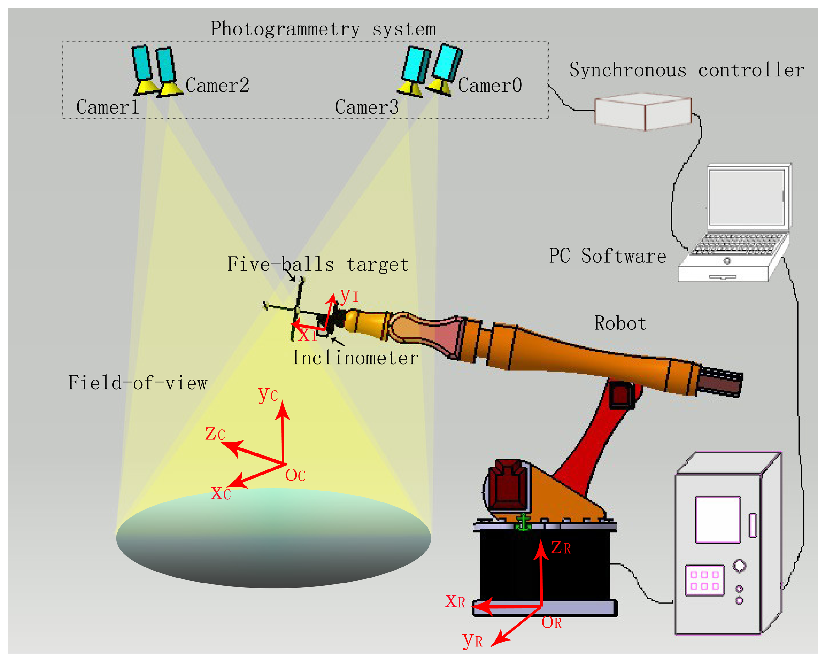
The conventional robot system cannot decrease the pose error at the control level due to the open-loop control architecture and simplified control laws. Instead of open-loop robot systems, the multiple-sensor combination measuring system (MCMS) presented in this paper sets up a closed-loop measurement system to improve the pose accuracy of the robot. As shown in Figure 1, the described system is made up of a series robot, an industrial photogrammetry system, a digital inclinometer and the PC software. As we know, the excellent measurement performance is achieved through the use of highly sophisticated components. In this paper we adopt a 6 DOF robot, whose repeatability accuracy is 10−3 mm. This robot is offered by KUKA Co., Ltd. (Shanghai, China) and its model is KP 5 arc. We also choose a high precision industrial three-dimensional photogrammetry system to dynamically track and measure the robot pose in real time. The photogrammetry system is composed of 4 motion-sensitive CCD cameras set on top of the robot. We also adopt a high accuracy digital inclinometer LE-30, whose accuracy is 0.01°. The inclinometer can rapidly measure both the angle of the pitch and yaw at a 20-ms frequency, and it can be set up on the robot manipulator to measure the attitude angle in real time. However, only possessing highly sophisticated instruments is not enough; the pose accuracy will be improved through fusing the redundant data of the sensors. These data should be converted by the coordinate transformation matrix previously.
2.2. Method of Data Fusion
As is well known, the primary aim of the sensor fusion is to improve the accuracy by using the redundant information gathered from multiple sources [9]. Since the construction of the MCMS, the sensor fusion is suitable to apply in this system. Currently, a number of different types of data fusion methods are being used in industry, such as the Wiener filter, constrained least squares filter, α-β filter, α-β-γ filter, Kalman filter [10], linear minimum variance fusion algorithm, etc. The Kalman filter (KF), first proposed in 1960 by Kalman [11], has been successfully used in the Apollo moon flight and C-5A aircraft navigation systems. Walker and Harries [12] improved the system robustness and adaptability in the mobile robot area through KF and multi-sensor fusion. The multi-sensor optimal information fusion algorithm in the linear minimum variance sense (MOIFA) is a geometric fusion method that was developed by Nakamura [13] and has been enhanced by Elliot et al. [14]. A demonstration of its use can be seen in [15], where the method was applied to an optical encoder and a camera sensor [16]. The two methods allow improving the fusion accuracy significantly, so we choose both of them as the methods of data fusion in this paper. We will summarize them respectively in Sections 2.2.1 and 2.2.2.
2.2.1. Kalman Filter
The Kalman filter solves the optimal linear filtering problems on the basis of a minimum mean square error method. The present value of the signal can be calculated according to the prior predicted value and the latest observation data. The Kalman filter predicts the value through a group of state equations and recursive methods. This recursive solution usually is expressed in the form of the predicted value. The following Equations (1)–(5) are the recursion formulas of the Kalman filter:
Substituting p(0) into Equation (4), we obtain p(1/0). Substituting p(1/0) into Equation (3), we obtain H (1). Substituting H (1) into Equation (1), we obtain X (1) in the condition of the minimum mean square error. At the same time, substituting p (1/0) into Equation (5), we obtain p (1). Then, we obtain p (2/1) by p (1), H (2) by p (2/1) and X (2) by H (2), the as same as above, and so on. Therefore, the predicted value at time k can be calculated.
In this paper, we only take into account the position accuracy of the robot. Two sensors, the photogrammetry system and the series robot, are utilized. Y1(k) is the observation value at time k of the photogrammetry system. Y2(k) is the observation value at time k of the robot, and X1(k) is the predicted value at time k of the photogrammetry system. X2(k) is the predicted value at time k of the robot. Xf(k) is fused by X1(k) and X2(k) with the weighting matrix W, which is determined by the typical accuracy values of the measuring instruments. Following is the principle of data fusion:
Xi is the three-dimensional coordinate of the predicted value with the i-th sensor. It usually can be expressed by means of a function of θ as Xi = f(θi), and θ is a multi-dimensional vector. A predicted value with additive noise can be represented as Xi = f(θi+δθi), where δθi represents the additive noise. Equation (6) is deduced by Taylor expanding Xi and neglecting the quadratic term.
Assuming a Gaussian distribution for the noise gives . Combining Equation (6), the mean and covariance of Xi are:
The weight matrix is defined as W = (W1W2…Wn), and n is the number of the sensors. The fusion value at time k combines multiple measurements by the weighted average:
Using Equations (6)–(11), the covariance matrix becomes:
Wi can be solved by means of Lagrange's method. The solving process is detailed in [13]. The weighting matrix is given to be:
In this paper, W1 and W2 represent the weighting matrices of the photogrammetry system and the series robot separately. According to Equation (9), the fused result at time k is:
2.2.2. Multi-Sensor Optimal Information Fusion Algorithm
The optimum fused value of the spatial coordinates for the robot position can be calculated as shown in Equation (15). “The optimum value” means the minimum variance unbiased estimate of the fused result X̂.
The covariance of Xi is given to be:
The fused covariance of X̂ is given below:
It obviously can be deduced from Equation (19) that V(X)−1 > Vi(X)−1; then V(X) < Vi(X). This proves that the fusion accuracy is better than the local accuracy.
3. Experiments and Discussion
To improve the accuracy of a robot manipulator, there are two steps in this paper. Firstly, the accuracy of a robot manipulator can be improved through the calibration for the kinematics parameters of the robot by the photogrammetry system. In addition, through calibrating the kinematics parameters of the robot, we can obtain a transformation relationship between the coordinate system of the photogrammetry system and robot. This makes the base coordinate system of the robot be a local unified coordinate system. Secondly, using the pose data of the calibrated robot and the online measurement of the multi-sensor combined measurement system (MCMS), three kinds of measurement data can be obtained. They are from the calibrated robot, photogrammetry system and inclinometer. The result can be improved by fusing these redundant data through KF and MOIFA. Therefore, four experiments are designed in this paper. Firstly, as an important part in MCMS, since the photogrammetry system directly monitors the robot pose, the accuracy of the photogrammetry system is crucial to the whole measurement system. The measurement errors of the photogrammetry system often appear to be due to the distortion on the edge of the FOV and the mistaken identity to the target. Therefore, it is necessary to research the repeatability accuracy of the photogrammetry system in its FOV, which is detailed in Section 3.1. Secondly, to improve the pose accuracy of the robot, the primary work is the calibration of the robot. Therefore, the experiment using the photogrammetry system to calibrate the robot is designed in Section 3.2. Thirdly, to observe the effect of the two data fusion methods, we design a simulation in Section 3.3. At last, in Section 3.4, a lab experiment is designed for verifying the result of the simulation. In this paper, all accuracy values (simulations and measurements) are given through the “three-sigma rule”, which is a method of eliminating the gross error by thrice the standard error in the theory of errors.
3.1. Repeatability Precision of Photogrammetry System
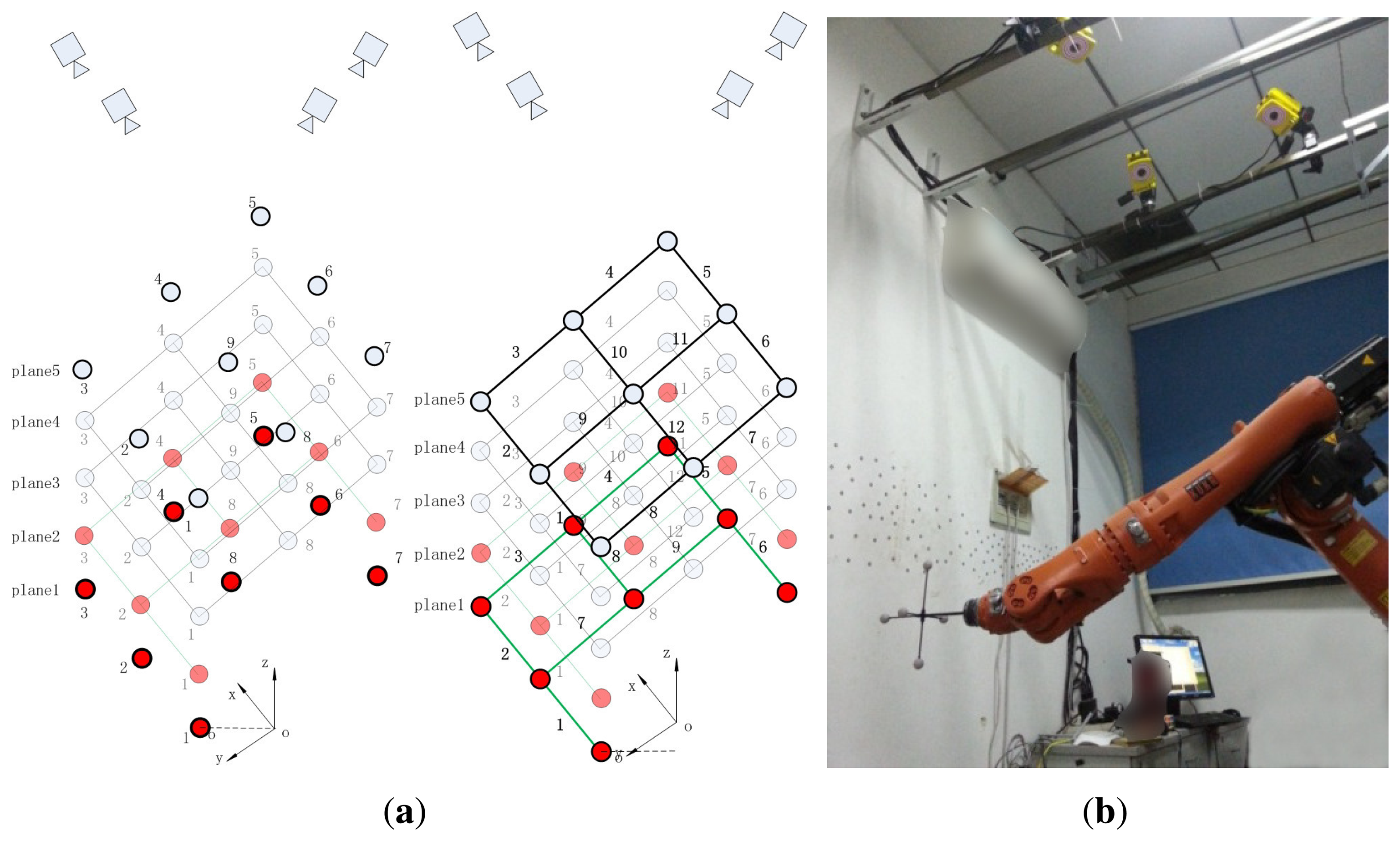
One of the ways to improve the photogrammetry system accuracy is to search for the optimal range of the FOV. As shown in Figure 2a, in order to test the accuracy of the photogrammetry system in the FOV, an experiment is designed as follows. The space of 1 × 0.8 × 1 m is divided into five planes from bottom to top, each of which contains 8∼9 points. Then, 9∼12 lines are formed through connecting the adjacent points. We move the robot manipulator to these points sequentially, and the photogrammetry system measures the coordinates of each point five times. In this paper, the laser tracker offered by FARO Co., Ltd. measures all points three times, and the result is used as the reference value. The FARO Xi laser tracker in the lab, whose uncertainty of the absolute distance meter (ADM) is 10 μm + 1.1 μm/mL, has been verified by the National Metrology Institute of China (NIM CDjx2008-0782). The measurement of the lines is similar as the points. The image of the experimental field is shown in Figure 2b.
3.1.1. Results of the Repeatability Precision of the Photogrammetry System
As shown in Table 1, the standard deviations of the position for 43 points are calculated by five groups of data, where δx,δy,δz are the standard deviations of three dimensions. Due to space limitations, we extract the data of Planes 1 and 5. δd is the compound standard deviation of δx,δy,δz.
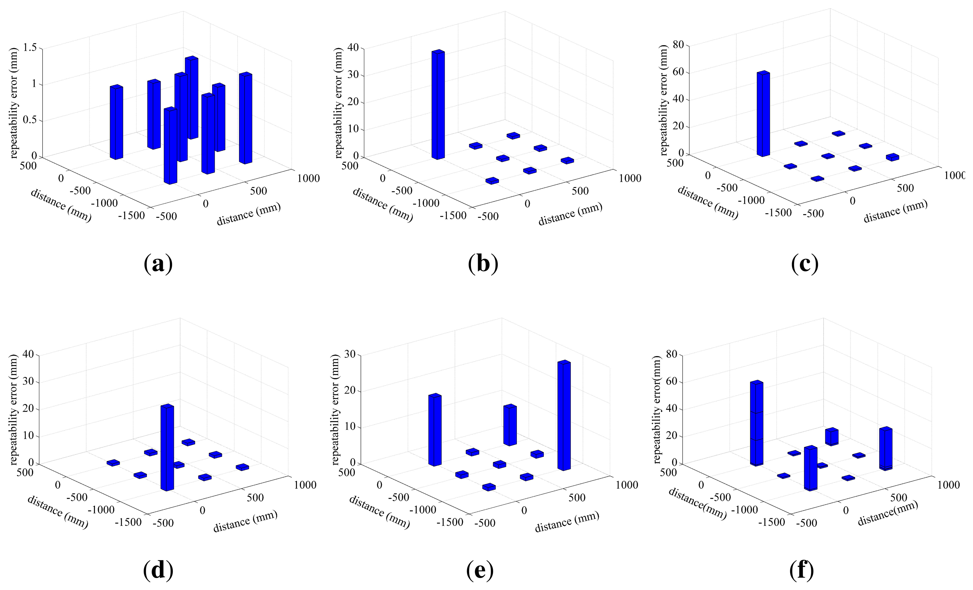
In order to show the distribution of the repeatability error in the FOV of the photogrammetry system, the histograms of the standard deviation are drawn in Figure 3. Figure 3a–e shows the error of Planes 1∼5, and Figure 3f shows the merged errors of all planes.
Some phenomena are observed in Figure 3. Firstly, the maximum error appears at the corner of each plane, such as Points 1, 3, 5, 7. Their merged errors are much larger than the other points, as shown in Figure 3. Except for these cornered points, the errors of the rest of the points are almost similar. Secondly, with the decreasing of the distance between the plane and the camera, the values and the number of the errors increase. Thirdly, the errors in the direction of x and z are smaller than y.
In this paper, TENYOUNfull body motion capture 3DMoCap-GC130 is used as a visual sensor. It takes more than 6 mm of prime lens as the optical lens of the camera. Its measurement range is more than 1 × 1 × 1 m. As we known, the FOV of the camera will enlarge with increasing of the photograph distance. The size of Plane 5 is 1 × 0.8 × 1 m, which can be considered to be the range close to the limitation of the measurement range. Plane 1, the length size of which is 1 × 0.8 × 2 m, is in a reasonable measurement range. Therefore, the error of Plane 5 is the largest in all planes and that of Plane 1 is the smallest. The result in Table 1 and Figure 3 shows that the repeatability error in the range of 1 × 0.8 × 1 ∼ 2 × 0.8 × 1 m has higher accuracy. The best accuracy is in the center of the range, the average values of which are δx = 0.124 mm, δy = 0.997 mm, δz = 0.272 mm, δd = 1.045 mm.
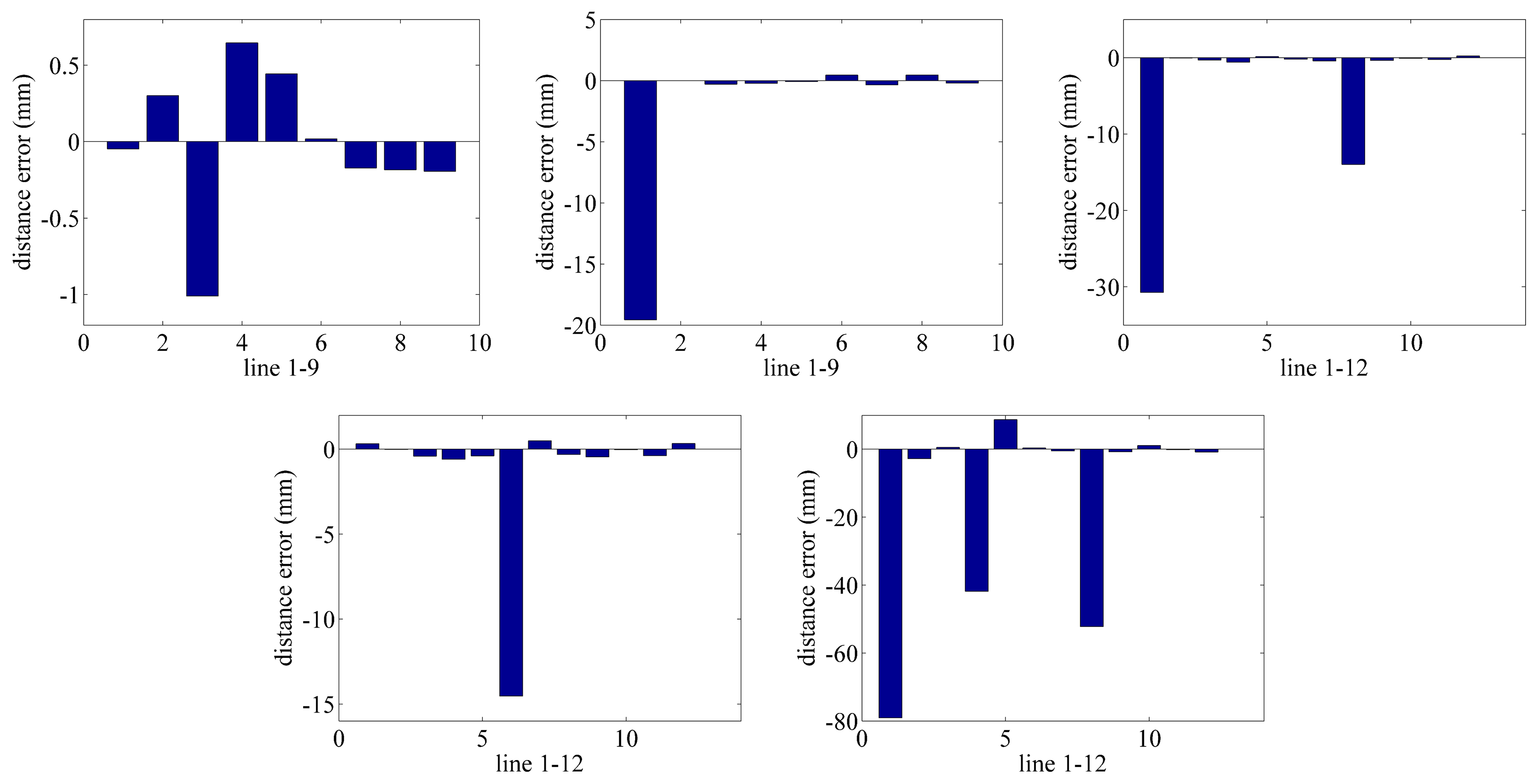
Secondly, we discuss the situation of the lines. As shown in Table 2, the standard deviations of 54 lines are calculated in comparison to the data of the laser tracker. Similarly, we select the data of Plane 1 and Plane 5. dl is the length measured by the laser tracker, and dc is the length measured by the photogrammetry system. Δd is the difference of the laser tracker and the photogrammetry system. The errors of the lines of each plane are drawn in Figure 4.
From Table 2 and Figure 4, we can find that the error of the lines has a similar phenomena as the points. The error of the lines increases with the decreasing of the distance between the plane and camera. The peak of the error appears in Lines 3, 4, 6, 8, which connect to the corner Points 1, 3, 5, 7. Accordingly, a conclusion can be drawn that the accuracy of the photogrammetry system is much higher in the range of 1 × 0.8 × 1 ∼ 2 × 0.8 × 1 m. The best accuracy of the lines is located in the center of the FOV, and its average value is Δd = 0.478 mm.
Therefore, the photogrammetry system can be used as the calibration instrument. The measured data also can be used as the feedback data to compensate for the errors of the robot in its effective measurement range.
3.2. Calibrating Method for the Robot
One of the ways to improve the pose accuracy for the robot manipulator is to calibrate the kinematics parameters of the robot. The photogrammetry system is used to monitor the pose of robot, so that it is reasonable to calibrate the robot by means of it. This paper proposes a calibrating method for the position error of the robot that is based on the D-H model. The first step of this method is to build a model of the coordinate transformation between the coordinate system of the photogrammetry system and the robot. Then, a kinematics parameter model of the robot manipulator is established according to the differential equation of the kinematics parameters error for the robot axes. The measured data of the photogrammetry system are converted into the coordinate system of the robot. Through comparing with the converted measured data, the parameters of the robot, such as the robot kinematics parameter, target installation error and transferred error of coordinate system, can be calibrated. A simple description of the main principle is shown below. The details of the calibrated method are shown in [17,18].
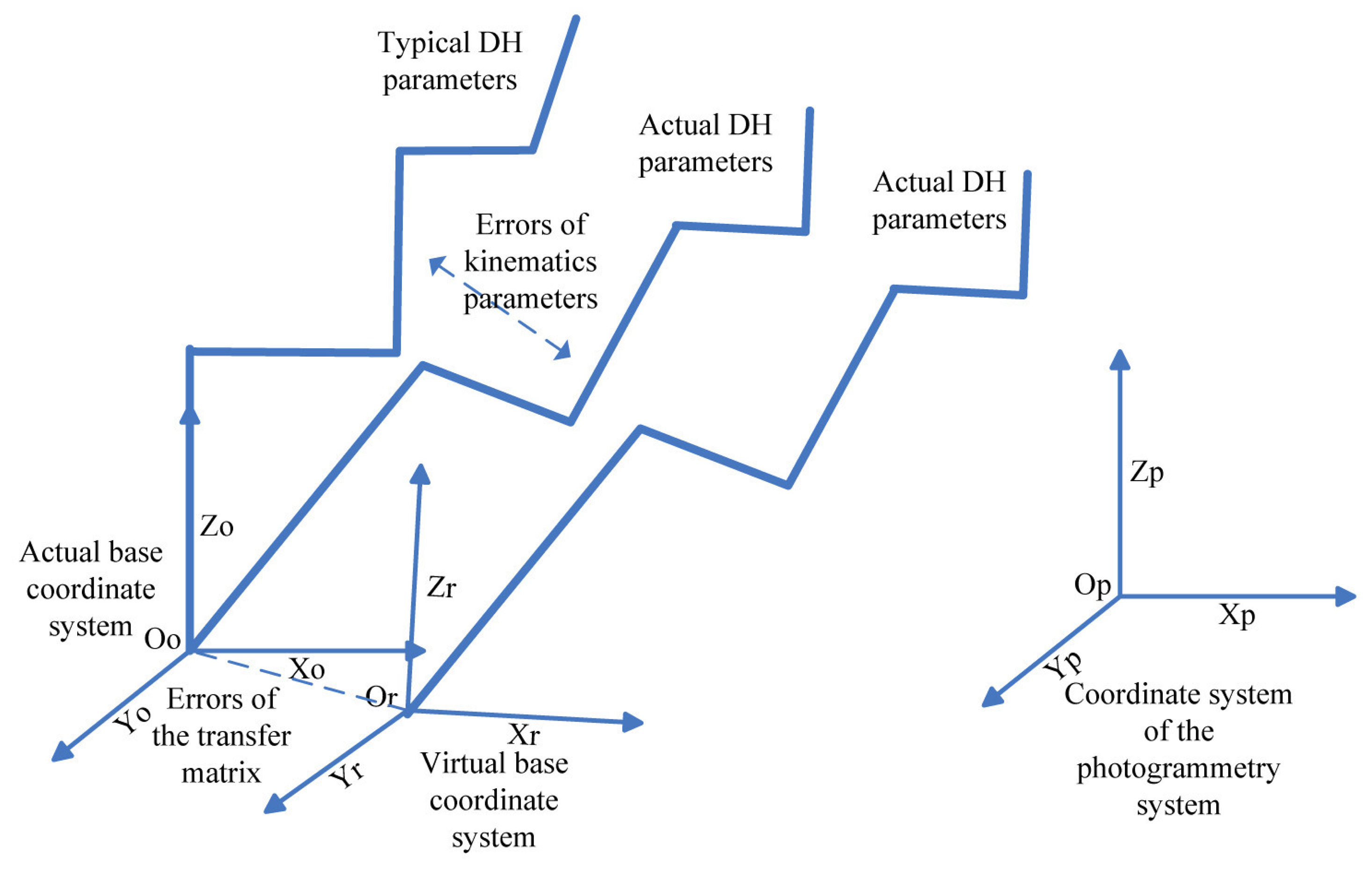
Figure 5 shows a simple model of the robot calibration. OpXpYpZp is the coordinate system of the photogrammetry system. OoXoYoZo is the actual base coordinate system of the robot. OrXrYrZr is the virtual base coordinate system of the robot measured by the photogrammetry system. The difference between the OoXoYoZo and OrXrYrZr is caused by the errors of the transfer matrix.
In order to obtain the position error of the robot, we must unify the coordinate systems of the photogrammetry system to the robot firstly. Assume is the transfer matrix from the coordinate system of the photogrammetry system OpXpYpZp to the virtual base coordinate system of the robot OrXrYrZr. Rotating Axis 1 of the robot with a certain degree, the photogrammetry system can obtain a group of data. Fitting the data, we obtain the vector of the direction z, which is the third component of . Similarly, the vector of the direction x, i.e., the first component of , can be obtained by rotating Axis 2 of the robot. Then, the vector of the direction y, i.e., the second component of , can be calculated by the cross-product of vector z and x. The translation vector (x, y, z) also can be fitted by the data.
Suppose that the error model of the transfer matrix from the OrXrYrZr and OoXoYoZo is expressed as Equation (20):
In addition, the cooperation target of the photogrammetry system, which is set up at the end axis of the robot, should be considered as an additional axis, Axis 7. Therefore, the transfer matrix from Axis 6 to Axis 7 is shown in Equation (21).
Therefore, the transfer matrix from the coordinate system of the photogrammetry system to the coordinate system of the robot manipulator is shown in Equation (22).
Assume is the pose of a certain point in the coordinate system of the photogrammetry system, where r1p ∼ r9p are the attitude parameters and pxp ∼ pzp are the position parameters. The converted pose of this point from the coordinate system of the photogrammetry system to the coordinate system of the robot manipulator can be obtained by calculation of Br = T · Bp using Equation (22). Then, the Z-Y-Z Euler angles (ϕ, θ, ψ), which express the attitude angles of the robot manipulator, can be obtained as shown in Equation (23).
The link parameters of the robot are the most significant impact factors on the position error of the robot. In the D-H model, they are the length of the link a, the displacement of the link d, the angle of rotation α and the link angle of each axis θ. In this paper, we adopt a series robot of six axes, so we can totally obtain 24 kinematics parameters Δa1∼4, Δd1∼4, Δα1∼4, Δθ1∼4. In addition, the transfer matrix from the coordinate system of the robot tool-center-point (TCP) to the end axis of the robot has nine rotation and translation error variables, as Equation (20) shows. Therefore, there are 33 parameters of the robot that need to be calibrated.
According to the distance error model of a series robot [17], the relationship of the distance error and position error is shown as Equation (24).
Because of the impact of four link parameters of the robot, it will cause the position error for the adjacent axes of the robot , which can be expressed as Equation (25).
If each of the two adjacent axes are influenced by the link parameters, the transformation from the base coordinate system of the robot to the coordinate system of the robot manipulator can be expressed as Equation (26). In this paper, N = 6.
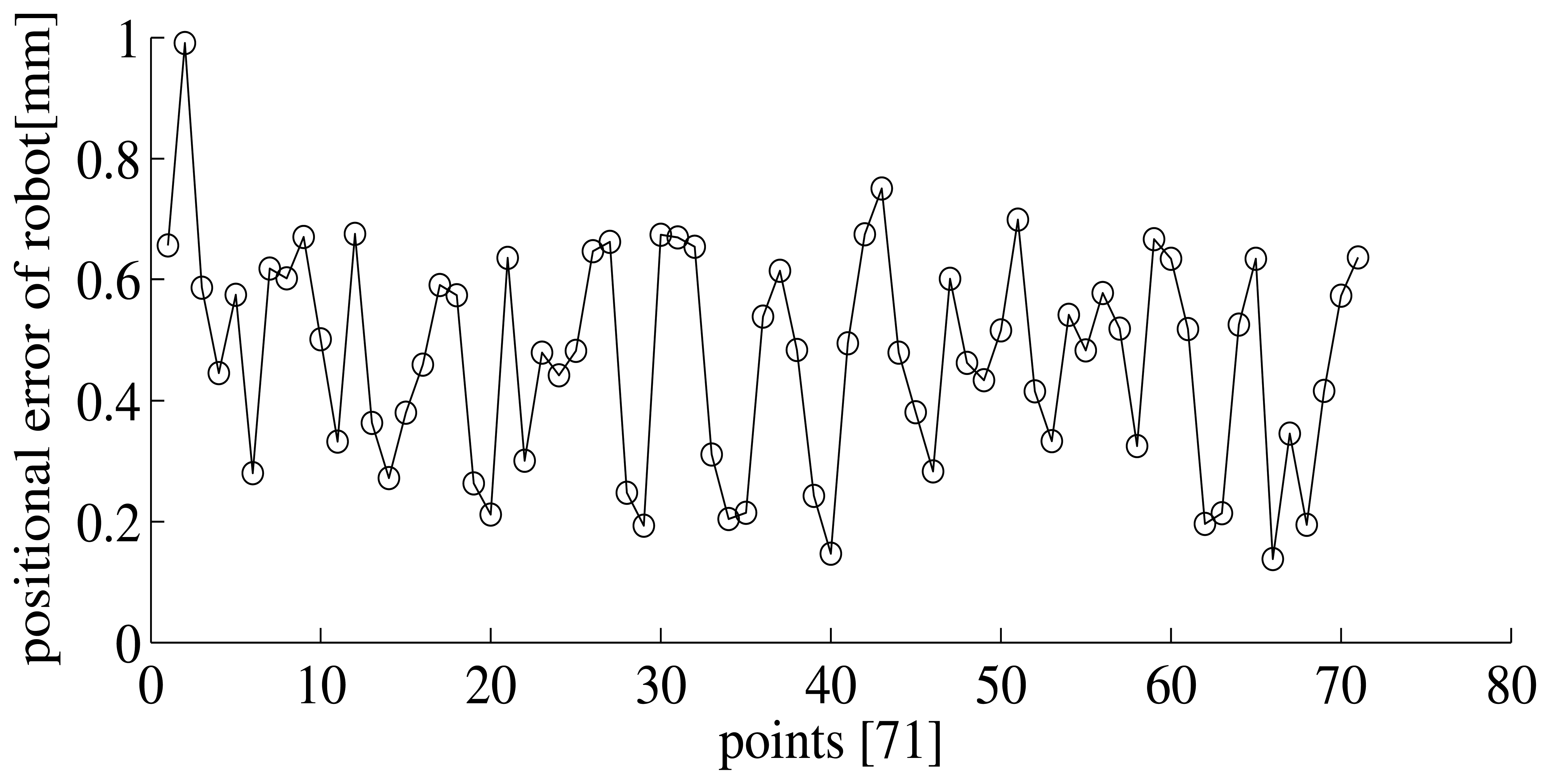
After calibrating by the photogrammetry system, the position error of the robot can be less than 1 mm. Figure 6 shows the position error of 71 points.
3.3. Simulation Test of the Sensor Data Fusion Methods
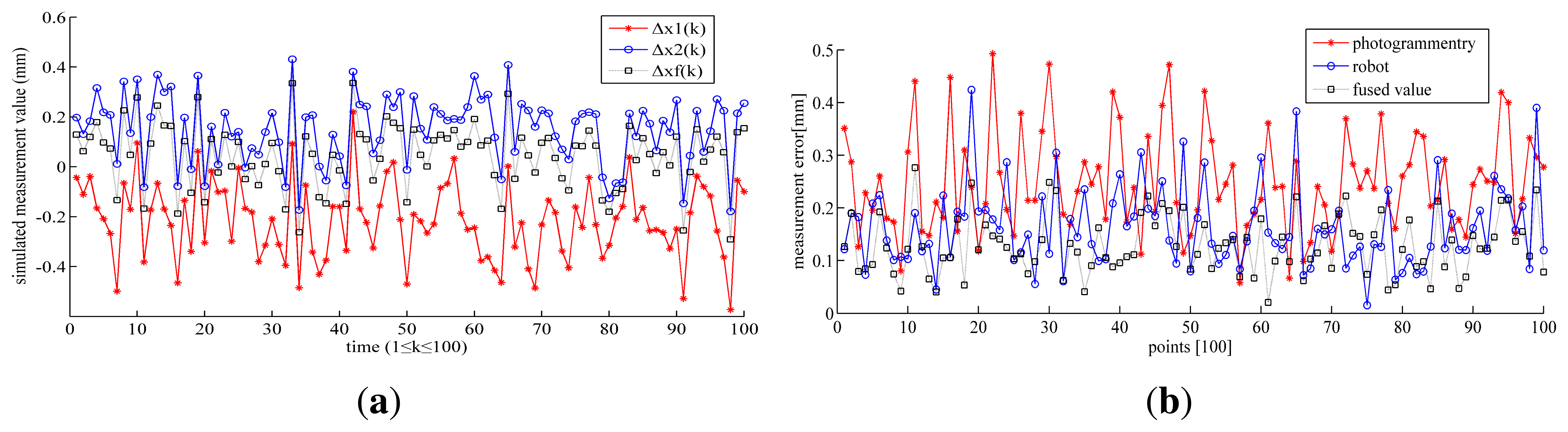
In terms of the position of the robot manipulator, there are two kinds of measurement data: one is obtained from the photogrammetry system and the other one is from the encoder of the robot. We propose two sensor data fusion methods to fuse the two kinds of position data. In order to compare the two methods, a simulation test is developed in MATLAB. One-hundred random points are created in a space of 100 × 100 × 100 mm to simulate the actual positions of the robot. For the purpose of simulating the actual value, each point is mixed with an error. It follows the normal distribution, which is determined by the typical value δ of the measured instruments. In this paper, the typical accuracy values of the photogrammetry system are δxc = δyc = δzc = 0.15 mm. The typical accuracy values of the robot are δxr = 0.157 mm, δyr = 0.087 mm, δzr = 0.043 mm. The typical values are calibrated by the FARO Xi laser tracker. Then, 100 points are fused by using KF and MOIFA.
In the first method, the simulated measured value of the photogrammetry system and robot, Y1(k) and Y2(k), are input into KF, as described in Equations (1)–(5), to obtain the estimated state variables, X1(k + 1) and X2(k + 1). Then, they are fused using the weight matrix W described in Equation (14), which is determined by the Jacobian matrices and covariance matrices of the photogrammetry system and robot. The fused error using KF is drawn in Figure 7a. In the second method, the simulated value of the photogrammetry and robot are fused as described in Equations (15)–(17). The fusion errors of MOIFA are drawn in Figure 7b.
3.3.1. Results of the Simulation Test of the Data Fusion Methods
As shown in Table 3, Δx1, Δx2 are the estimated errors of the photogrammetry and robot after fusing by the KF method, respectively. Δxf is the fused error. ΔCM, ΔRB are the errors of the photogrammetry and robot, respectively. Δf is the fused error after fusing by MOIFA.
Since the photogrammetry system has a bigger typical accuracy value, the error of the photogrammetry system is bigger than that of the robot, as shown in Table 3. It is indicated in Figure 7a,b and Table 3 that either of the methods can reduce the error after the data fusion. Through calculating the data in Table 3, the error is reduced by 78.2% with KF and by 46.1% with MOIFA. As shown in Table 3, KF has smaller fused errors than MOIFA. In addition, KF can predict the state variables of next moment, which is suitable to be applied in the dynamic measurement and compensation. MOIFA can only analyze the ready-measured data. However, it will cause the hysteresis of the real-time compensation. It should be noted that the measuring range is 0∼100 mm in this experiment. KF is a linear filter, so that its fused error will be enlarged with increasing the measuring range. This will be verified in the lab experiment in Section 3.4.
3.4. Verified Experiment in the Lab
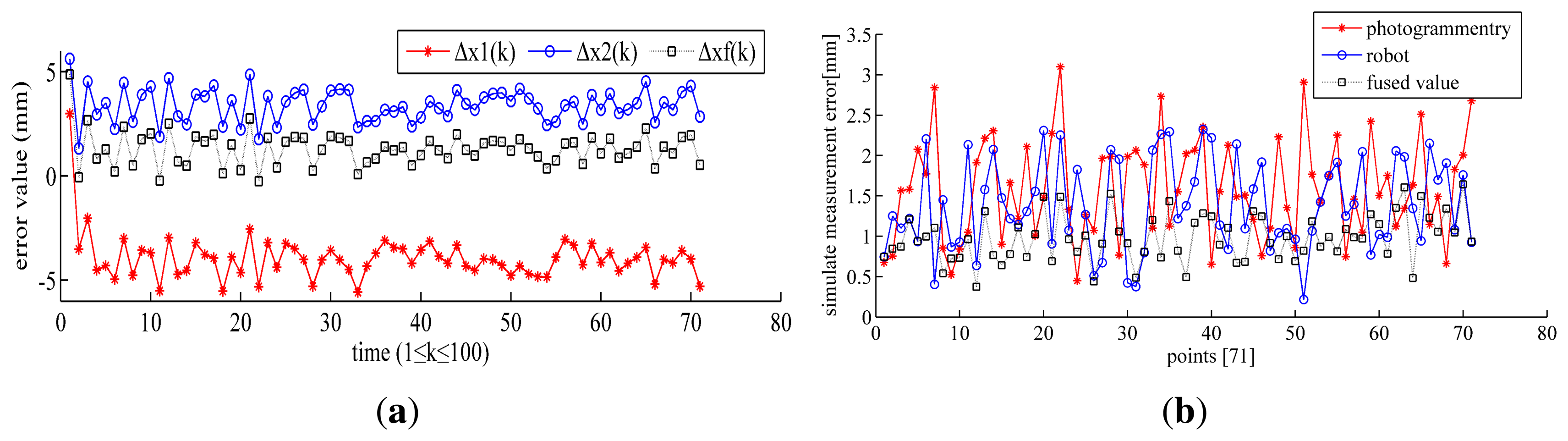
In order to validate the conclusion of the simulation test, a data fusion-verified experiment in lab is designed. For the purpose of measuring the pose of the robot manipulator, a five-ball target frame of the photogrammetry system and the inclinometer are set up at the end of the robot through a special fixture, as shown in Figure 1. Seventy six points are located on the surface of a 200-mm radius sphere, which is in the space of 1 × 1 × 1 m in the front of the robot. Obviously, these points must also be located in the effective measurement area of the photogrammetry system, as described in Section 3.1. For acquiring the stable data, the robot stays in each position for 7 s to offer enough measurement time for the photogrammetry system. Since the robot has been calibrated in Section 3.2, in this experiment, all data are converted into the base coordinate system of the robot. The measurement value of the FARO Xi laser tracker is used as the reference value. Then, 71 picked points are fused using KF and MOIFA.
The same as the process of the simulate experiment described in Section 3.3, the fused error using KF is drawn in Figure 8a, and the fused error using MOIFA is drawn in Figure 8b.
3.4.1. Result of the Verified Experiment in the Lab
The average values of the measurement error are shown in Table 4.
It is indicated in Table 4 that in the lab experiment, the errors of the photogrammetry system are bigger than that of the robot. This is because its typical value is bigger than the robot, that same as the simulation experiment shown in Section 3.3.1. The error of the photogrammetry system ΔCM in the lab experiment is smaller than the simulation test. This illustrates that the accuracy of the photogrammetry system in its effective FOV is improved, as we had tested in the repeatability experiment in Section 3.1.1. It is seen in Figure 8a,b and Table 4 that both of the fused methods can reduce the error after the data fusion. Through the data calculation in Table 4, the error is reduced by 67.3% with KF and by 38.2% with MOIFA. This is a little smaller than the results of the simulation, but both of them have common trends. However, the value of the fused error using KF is a little larger than the error of the simulation. The reason is that KF is a linear filter, which had been discussed previously in Section 3.3.1. Comparing to the other works, Yauheni and Jerzy of Warsaw University of Technology obtain the improved value of the positioning accuracy for the robot end-effector ΔL = 2.39 mm using the method of joint error mutual compensation. Li Junmin and Wang Jinge et al. improved the pose accuracy of the robot to 2.2 mm based on the unit quaternion and the prediction of the pose estimation accuracy. It is indicated that the multiple-sensor combination measuring system (MCMS) proposed in this paper has good performance for improving the pose accuracy of the robot.
Therefore, a conclusion can be made in comparison to the simulation that both of the data fusion methods can lead to the improvement of the results. MOIFA has more stable accuracy of the fusion, but it has no predicted function, which would cause hysteresis in the feedback control system of the robot. KF is widely applied in the areas of robotics and aviation. It possesses the predicted function of the next moment, which is suitable for real-time measurement and compensation. However, its predicted error would be enlarged with increasing measurement range, since it is a kind of linear filter. According to the features of the two data fusion methods, we can adopt KF to fuse data when dynamic and real-time measurement is needed, as well as when the measurement range is small. Otherwise, MOIFA can be adopted when the static and offline measurement is needed, as well as when the measurement range is large.
4. Conclusions
In this paper, we proposed a multi-sensor combination measuring system (MCMS) and two sensor data fusion methods to improve the pose accuracy of industrial robots. The advantage of this method is that it is automatic and does not involve environmental intervention. To ensure the accuracy of the measured sensor, this paper researched the repeatability precision of the photogrammetry system and the robot calibration by means of the photogrammetry system. The experimental results show that the best accuracy of the photogrammetry system is in the center of the FOV, which is the range of 1 × 0.8 × 1 ∼ 2 × 0.8 × 1 m. The position error of the robot manipulator is less than 1 mm after being calibrated by the photogrammetry system. In order to improve the accuracy of the robot pose, we propose two kinds of data fusion methods to fuse the redundant information gathered from the multiple sensors. Through comparing with the simulation and lab experimental results, KF possesses a predicted function of the next moment that is suitable for real-time measurement and compensation. However, its predicted error would be enlarged with an increasing measurement range, since it is a kind of linear filter. On the other hand, MOIFA possesses the stable accuracy of fusion, but it is not capable of the predicting function. This will cause hysteresis in the feedback control system of the robot. Therefore, both of the methods can reduce the pose error of the robot by 38%∼78%. The choice of method is dependent on the requirements of the measurement. The experimental and theoretical results provided the basis for an industrial application of the robot pose measurement and compensation. Future works will include the real-time transferring of data, online control and compensation for the pose of the robot manipulator.
Acknowledgements
This research was supported by the Natural Science Foundation of China (NSFC) No. 51275350 and the Specialized Research Fund for the Doctoral Program of Higher Education of China No. 20110032110045.
Author Contributions
Bailing Liu, Fuming Zhang and Xinghua Qu conceived and designed the experiments; Bailing Liu performed the experiments; Bailing Liu and Fumin Zhang analyzed the data; Xinghua Qu contributed analysis tools; Bailing Liu wrote the paper.
Conflicts of Interest
The authors declare no conflict of interest.
References
- Yauheni, V.; Jerzy, K. Application of joint error mutual compensation for robot end-effector pose accuracy improvement. J. Intell. Robot. Syst. Theory Appl. 2003, 36, 315–329. [Google Scholar]
- Jian, Y.Z.; Chen, Z.; Da, W.Z. Pose accuracy analysis of robot manipulators based on kinematics. Adv. Manuf. Syst. 2011, 201–203, 1867–1872. [Google Scholar]
- Du, G.; Zhang, P. Online serial manipulator calibration based on multisensory process via extended kalman and particle filters. IEEE Trans. Ind. Electron. 2014, 61, 6852–6859. [Google Scholar]
- Frank, S.C. The Method of Recovering Robot TCP Positions in Industrial Robot Application Programs. Proceedings of the 2007 IEEE International Conference on Mechatronics and Automation, Harbin, China, 5–8 August 2007; pp. 805–810.
- Hans, D.R.; Beno, B. Visual-model-based, real-time 3D pose tracking for autonomous navigation: Methodology and experiments. Auton. Robot 2008, 25, 267–286. [Google Scholar]
- Kaijen, H.L.; Pack, K.; Tomás, L.P. Robust grasping under object pose uncertainty. Auton. Robot 2011, 201–203, 253–268. [Google Scholar]
- Qu, W.W.; Dong, H.Y.; Ke, Y.L. Pose accuracy compensation technology in robot-aided aircraft assembly drilling process. Acta Aeronaut. Astronaut. Sin. 2011, 32, 1951–1960. [Google Scholar]
- Camille, S.C.; Rainer, S.; Frank, B.; Franck, S.M. Registration of arbitrary multi-view 3D acquisitions. Comput. Ind. 2013, 64, 1082–1089. [Google Scholar]
- Thomas, L. Close range photogrammetry for industrial applications. ISPRS J. Photogramm. Remote Sens. 2010, 65, 558–569. [Google Scholar]
- Ba, H.X.; Zhao, Z.G. A survey on mathematic models and methods of multisensor data fusion. Ship Sci. Technol. 2005, 27, 48–53. [Google Scholar]
- Kalman, R.E. A new approach to linear filtering and prediction problems. J. Basic Eng. 1960, 82, 35–46. [Google Scholar]
- Abidi, M.A.; Gonzalez, R.C. Data Fusion in Robotics and Machine Intelligence; Academic Press: Waltham, MA, USA, 1992; Volume 19, pp. 888–896. [Google Scholar]
- Nakamura, Y.; Zu, Y. Geometrical Fusion Method for Multi-Sensor Robotic Systems. Proceedings of the 1989 IEEE International Conference on Robotics and Automation, Scottsdale, AZ, USA, 14–19 May 1989; Volume 2, pp. 668–673.
- Langlois, D.; Elliott, J.; Croft, E.A. Sensor Uncertainty Management for an Encapsulated Logical Device Architecture, Part II: A Control Policy for Sensor Uncertainty. Volume 1–6, 4288–4293.
- Nandi, G.C.; Mitra, D. Development of a Sensor fusion Strategy for Robotic Application Based on Geometric Optimization. J. Intell. Robot. Syst. 2002, 35, 171–191. [Google Scholar]
- John, M.; Allan, S.; Manhtriet, H.; Arnold, F. Sensor Fusion of Laser Trackers for Use in Large-Scale Precision Metrology in Intelligent Manufacturing. Proc. SPIE Intell. Manuf. 2004, 5263. [Google Scholar] [CrossRef]
- Ren, Y.J. The Study on Main Body Calibration Technique of Measuring Robot; Tianjin University: Tianjin, China, 2007; pp. 71–76. [Google Scholar]
- Li, R.; Qu, X.H. Study on calibration uncertainty of industrial robot kinematics parameters. Chin. J. Sci. Instrum. 2014, 35, 2192–2199. [Google Scholar]


| Plane 1 | δx | δy | δz | δd |
| 1 | 0.046 | 0.929 | 0.303 | 0.979 |
| 2 | 0.119 | 0.872 | 0.246 | 0.914 |
| 3 | 0.128 | 1.058 | 0.242 | 1.093 |
| 4 | 0.218 | 0.800 | 0.325 | 0.891 |
| 5 | 0.106 | 1.189 | 0.229 | 1.215 |
| 6 | 0.075 | 1.028 | 0.275 | 1.067 |
| 7 | 0.064 | 0.972 | 0.283 | 1.015 |
| 8 | 0.231 | 1.126 | 0.272 | 1.181 |
| Plane 5 | δx | δy | δz | δd |
| 35 | 13.902 | 7.396 | 10.661 | 19.017 |
| 36 | 0.062 | 0.950 | 0.255 | 0.985 |
| 37 | 4.709 | 9.126 | 1.822 | 10.431 |
| 38 | 0.075 | 1.057 | 0.256 | 1.090 |
| 39 | 10.487 | 9.584 | 25.830 | 29.479 |
| 40 | 0.095 | 0.920 | 0.286 | 0.968 |
| 41 | 0.102 | 0.896 | 0.406 | 0.989 |
| 42 | 0.064 | 0.989 | 0.285 | 1.031 |
| 43 | 0.068 | 1.007 | 0.273 | 1.046 |
| Plane 1 | dl | dc | Δd |
| 1 | 400.202 | 400.249 | −0.047 |
| 2 | 400.482 | 400.179 | 0.302 |
| 3 | 500.253 | 501.264 | −1.010 |
| 4 | 500.140 | 499.492 | 0.647 |
| 5 | 400.794 | 400.350 | 0.443 |
| 6 | 400.509 | 400.491 | 0.018 |
| 7 | 500.325 | 500.498 | −0.172 |
| 8 | 400.399 | 400.583 | −0.184 |
| 9 | 500.112 | 500.306 | −0.193 |
| Plane 5 | dl | dc | Δd |
| 1 | 321.442 | 400.547 | −79.104 |
| 2 | 398.357 | 401.150 | −2.793 |
| 3 | 501.106 | 500.544 | 0.562 |
| 4 | 458.928 | 500.737 | −41.809 |
| 5 | 409.822 | 401.110 | 8.711 |
| 6 | 401.108 | 400.693 | 0.415 |
| 7 | 499.526 | 500.038 | −0.511 |
| 8 | 447.228 | 499.478 | −52.249 |
| 9 | 499.533 | 500.300 | −0.767 |
| 10 | 401.440 | 400.309 | 1.131 |
| 11 | 499.971 | 500.153 | −0.181 |
| 12 | 401.508 | 402.316 | −0.808 |
| Δx1 | Δx2 | Δxf |
| −0.198 | 0.139 | 0.043 |
| ΔCM | ΔRB | Δf |
| 0.240 | 0.156 | 0.129 |
| Δx1 | Δx2 | Δxf |
| −3.940 | 3.379 | 1.297 |
| ΔCM | ΔRB | Δf |
| 1.587 | 1.386 | 0.981 |
© 2015 by the authors; licensee MDPI, Basel, Switzerland. This article is an open access article distributed under the terms and conditions of the Creative Commons Attribution license ( http://creativecommons.org/licenses/by/4.0/).
Share and Cite
Liu, B.; Zhang, F.; Qu, X. A Method for Improving the Pose Accuracy of a Robot Manipulator Based on Multi-Sensor Combined Measurement and Data Fusion. Sensors 2015, 15, 7933-7952. https://0-doi-org.brum.beds.ac.uk/10.3390/s150407933
Liu B, Zhang F, Qu X. A Method for Improving the Pose Accuracy of a Robot Manipulator Based on Multi-Sensor Combined Measurement and Data Fusion. Sensors. 2015; 15(4):7933-7952. https://0-doi-org.brum.beds.ac.uk/10.3390/s150407933
Chicago/Turabian StyleLiu, Bailing, Fumin Zhang, and Xinghua Qu. 2015. "A Method for Improving the Pose Accuracy of a Robot Manipulator Based on Multi-Sensor Combined Measurement and Data Fusion" Sensors 15, no. 4: 7933-7952. https://0-doi-org.brum.beds.ac.uk/10.3390/s150407933