New Quality Control Algorithm Based on GNSS Sensing Data for a Bridge Health Monitoring System


Abstract
:1. Introduction
2. Quality Control Algorithm and Quality Measures
2.1. Least Squares Estimation and Outliers
- is only influenced by the random error of residuals, and
- is affected by outliers of residuals.
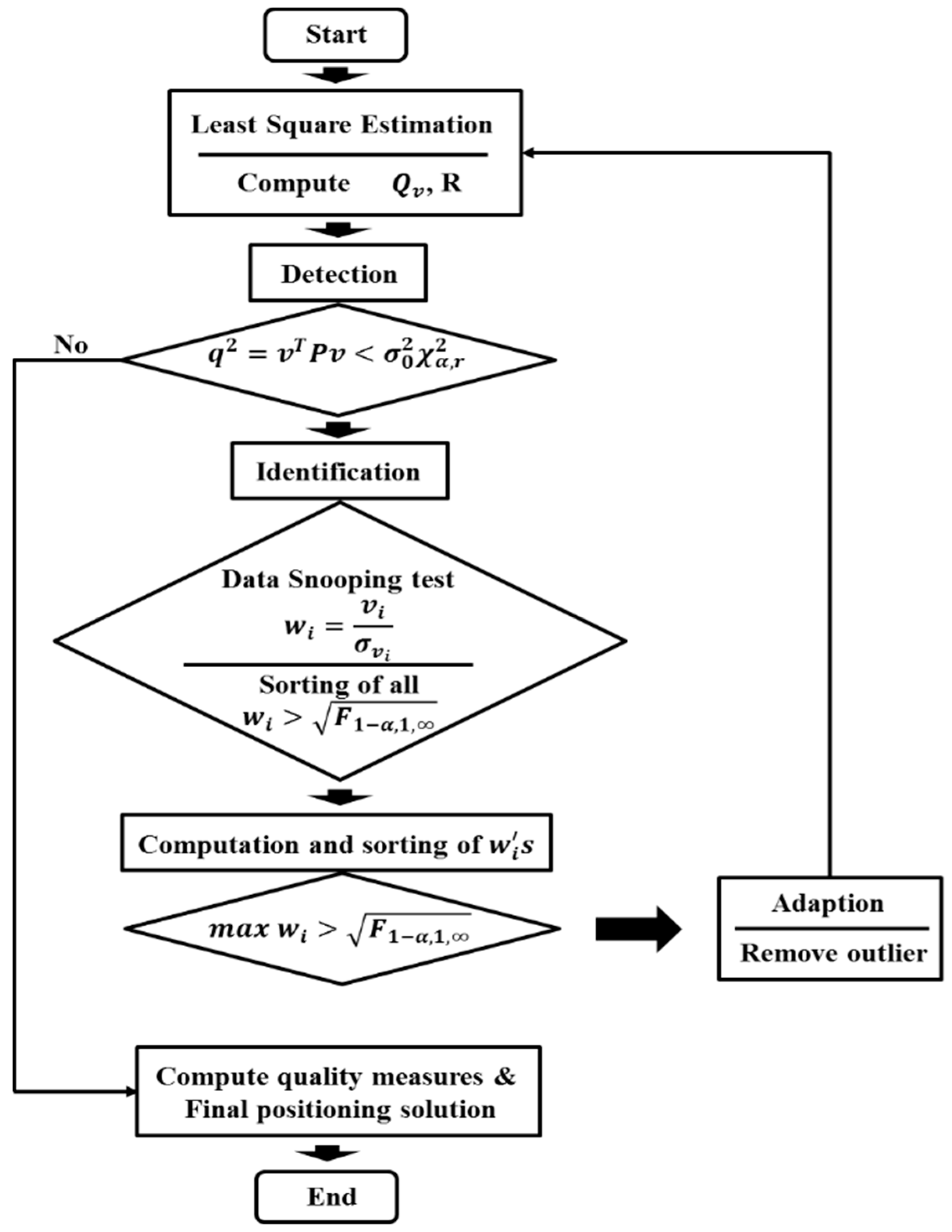
2.2. Quality Control Algorithm Procedure
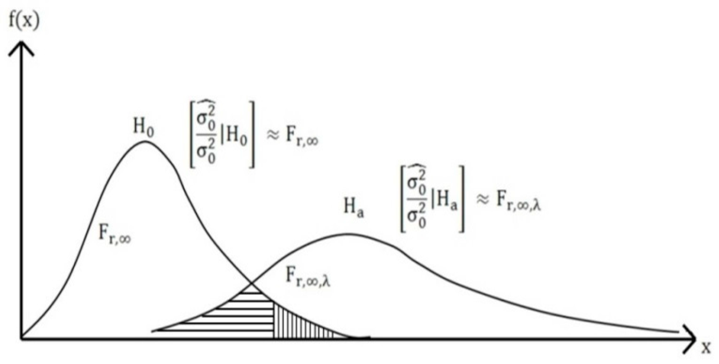
2.2.1. Detection
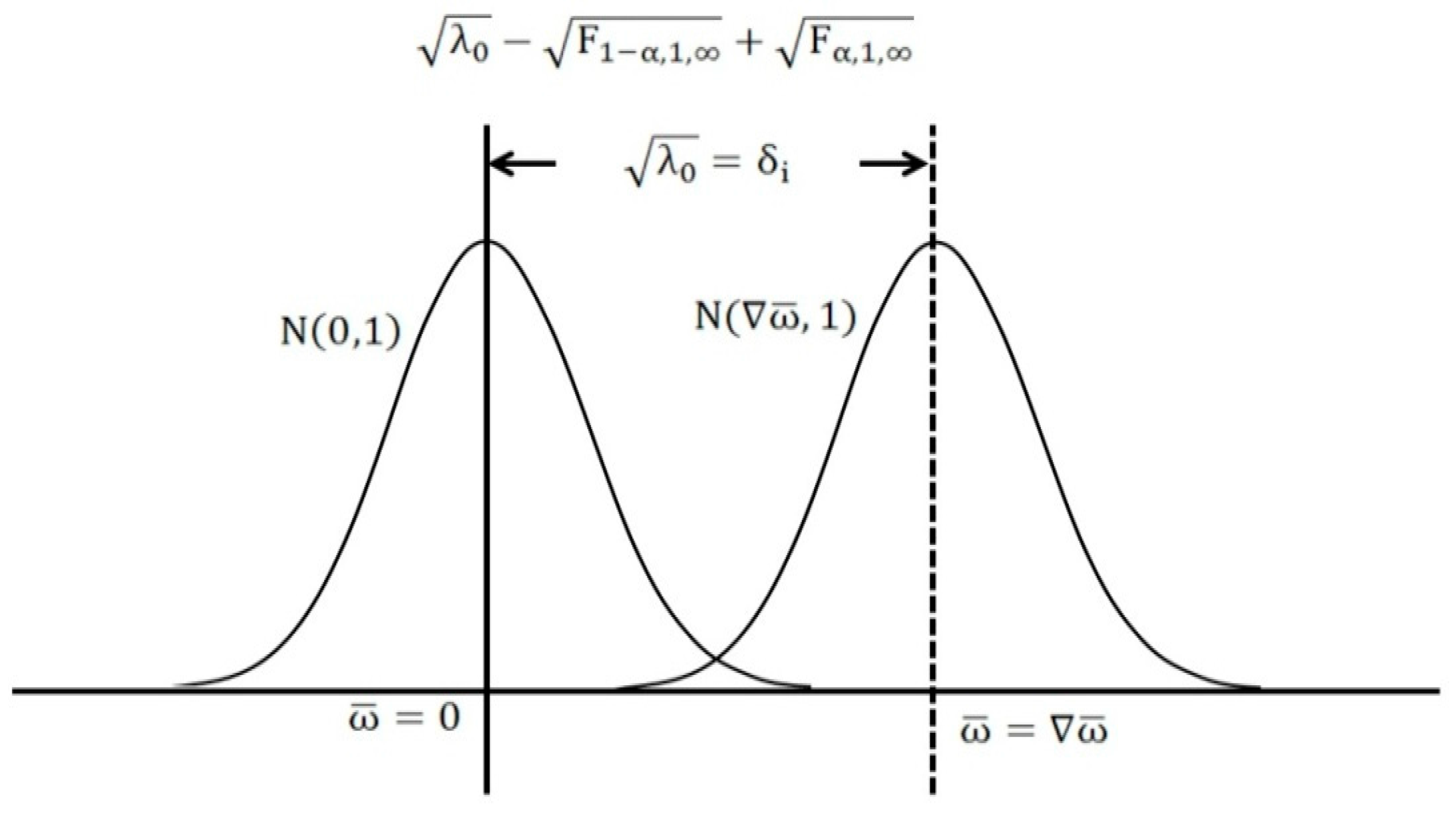
2.2.2. Identification
2.2.3. Adaptation
2.3. Quality Measures
2.3.1. Redundancy Number
2.3.2. Quality Dilution of Precision (QDOP)
2.3.3. Reliability
- -
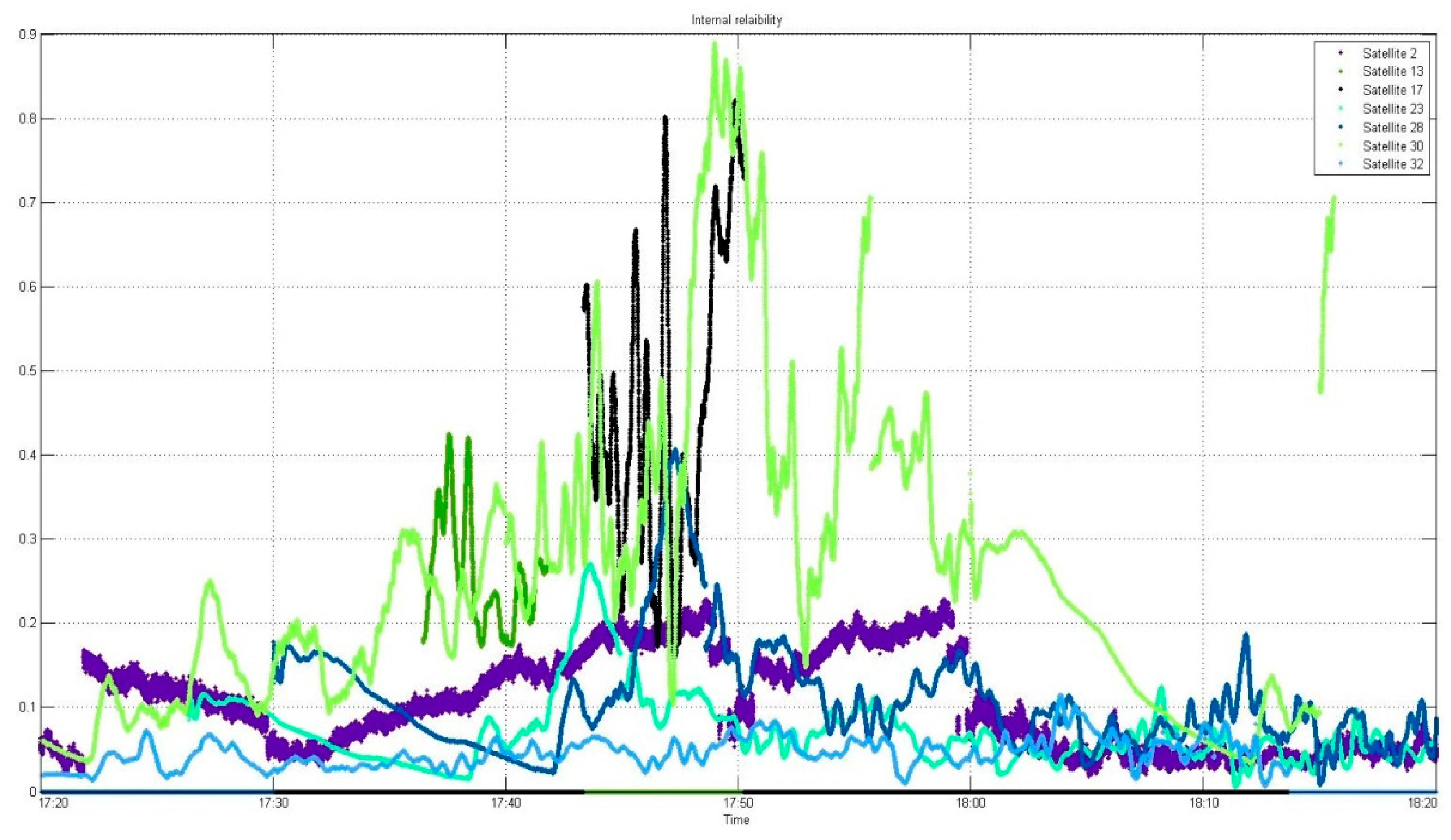
- Internal reliability
- -
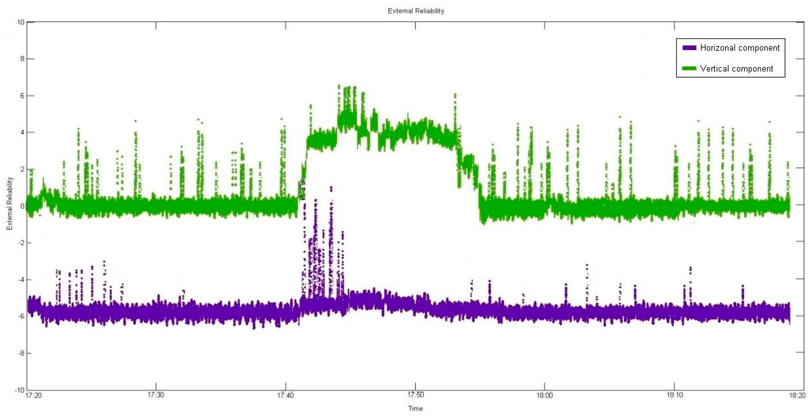
- External reliability
3. Bridge Experiment
3.1. Introduction
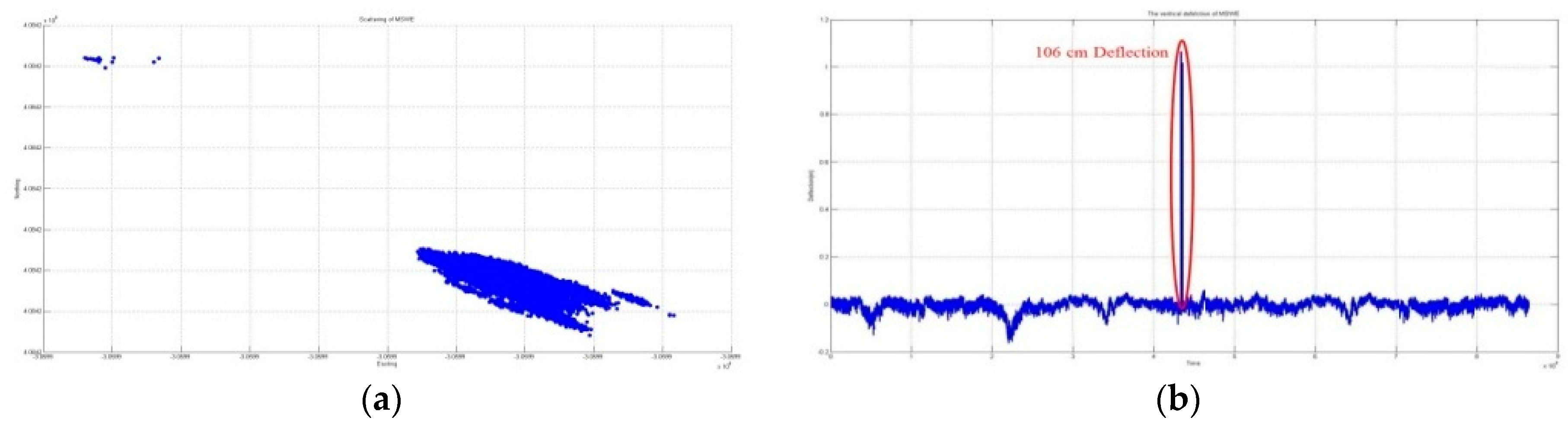
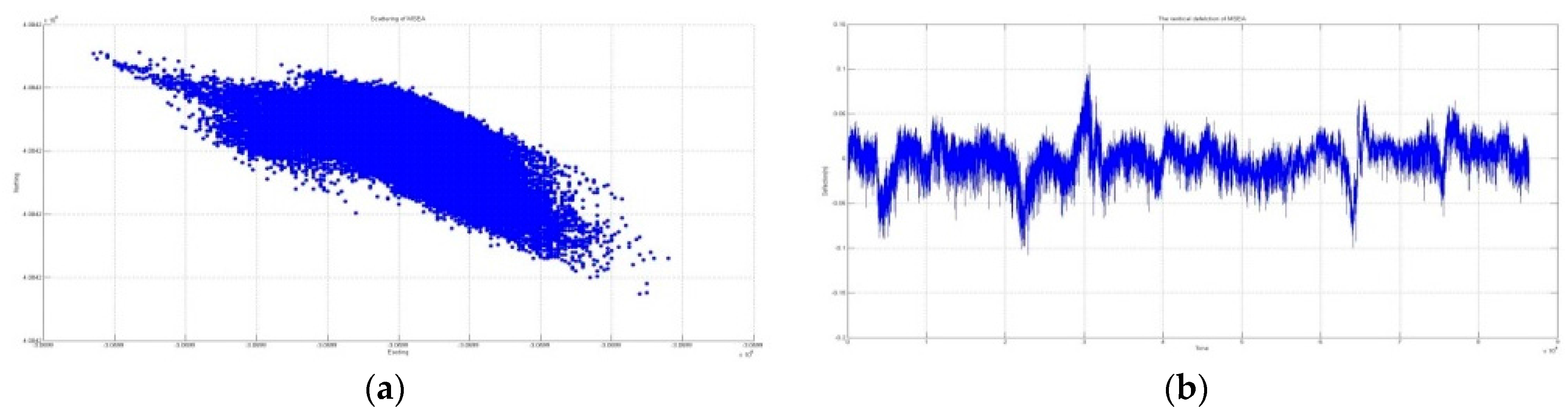
3.1.1. Evidence of Existing Outliers
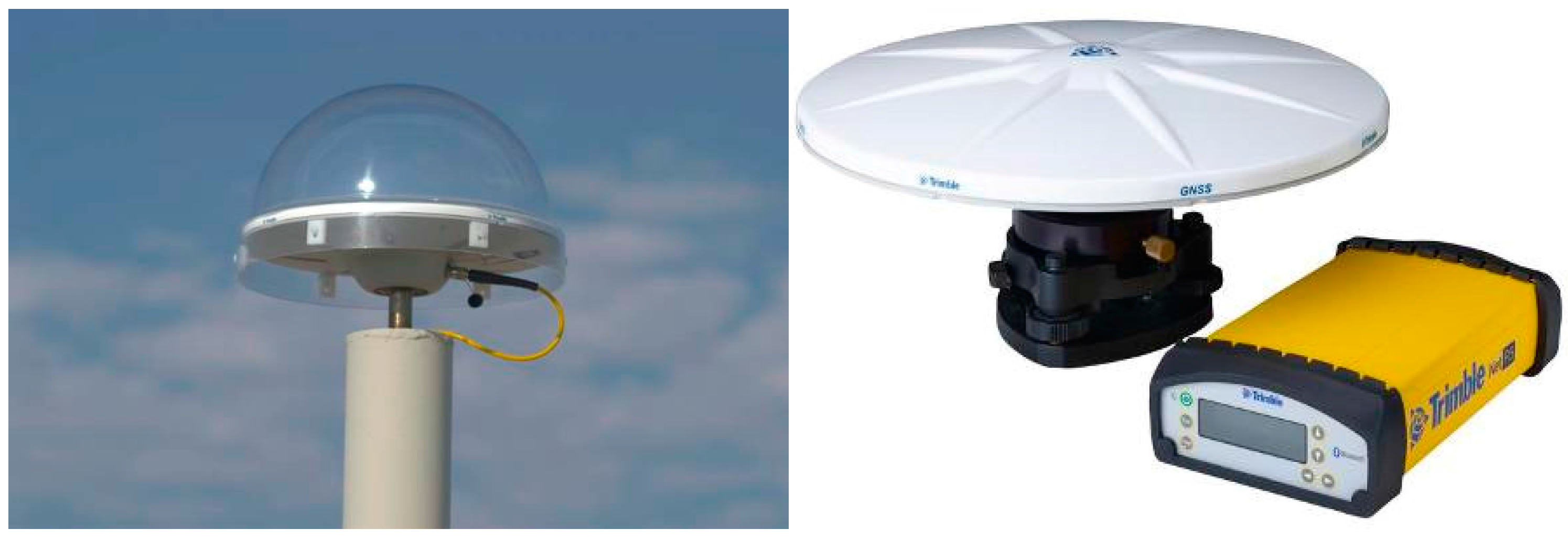
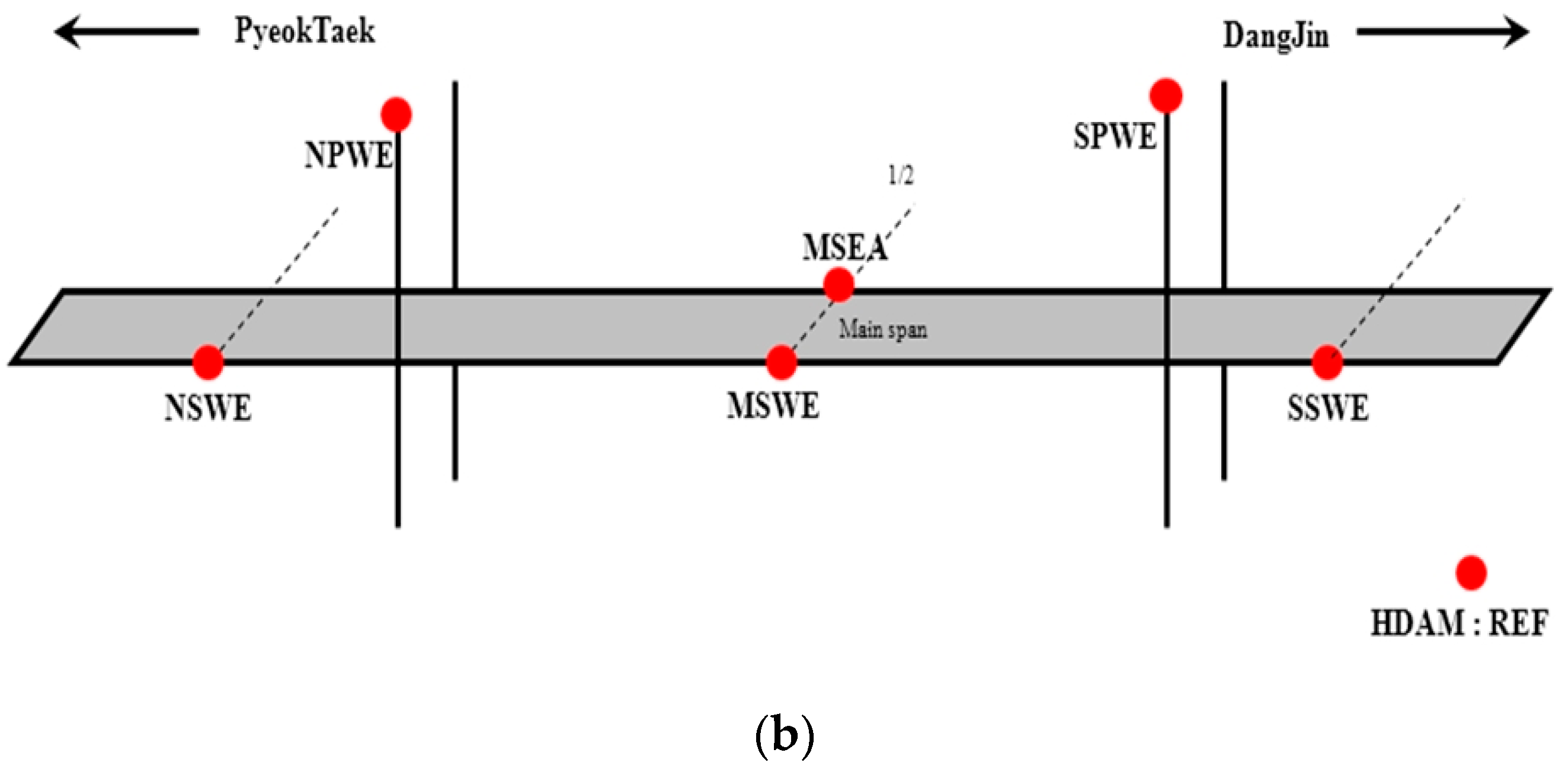
3.1.2. Test Description & Test-Bed
- -
- Test Description
- -
- Test-Bed
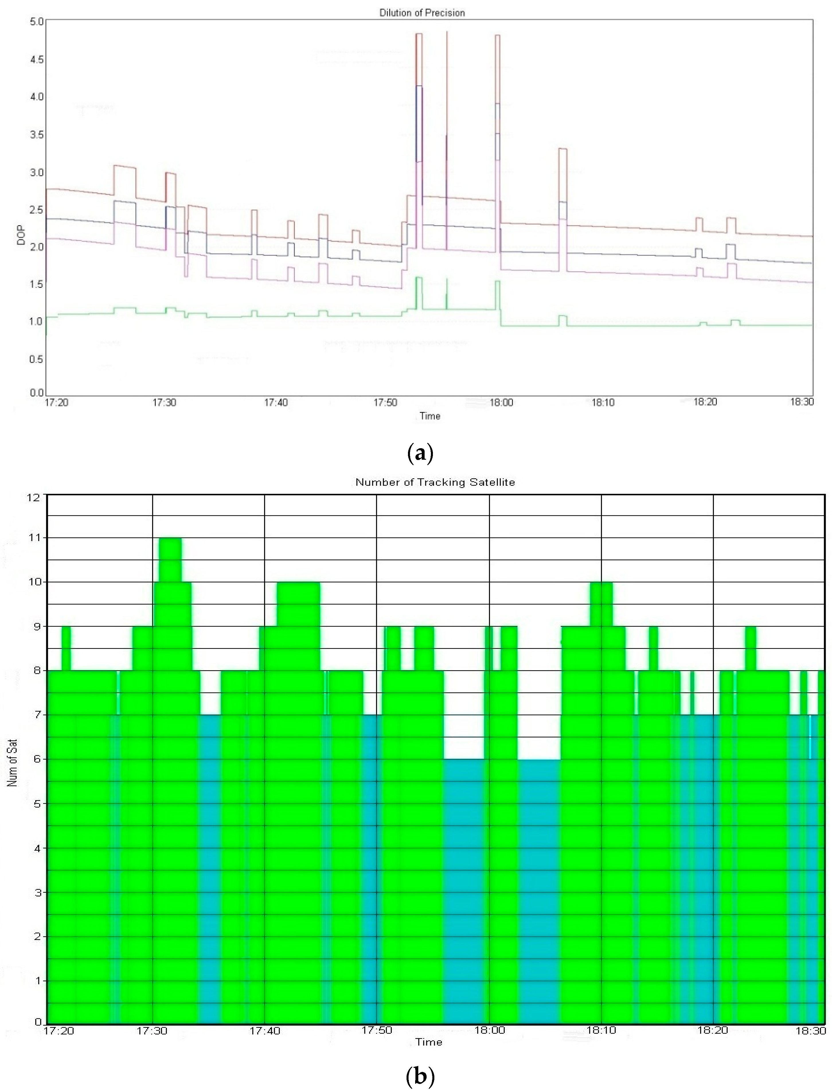
3.1.3. Pre-Analysis on the Status of GPS Signal
3.2. Quality Measures
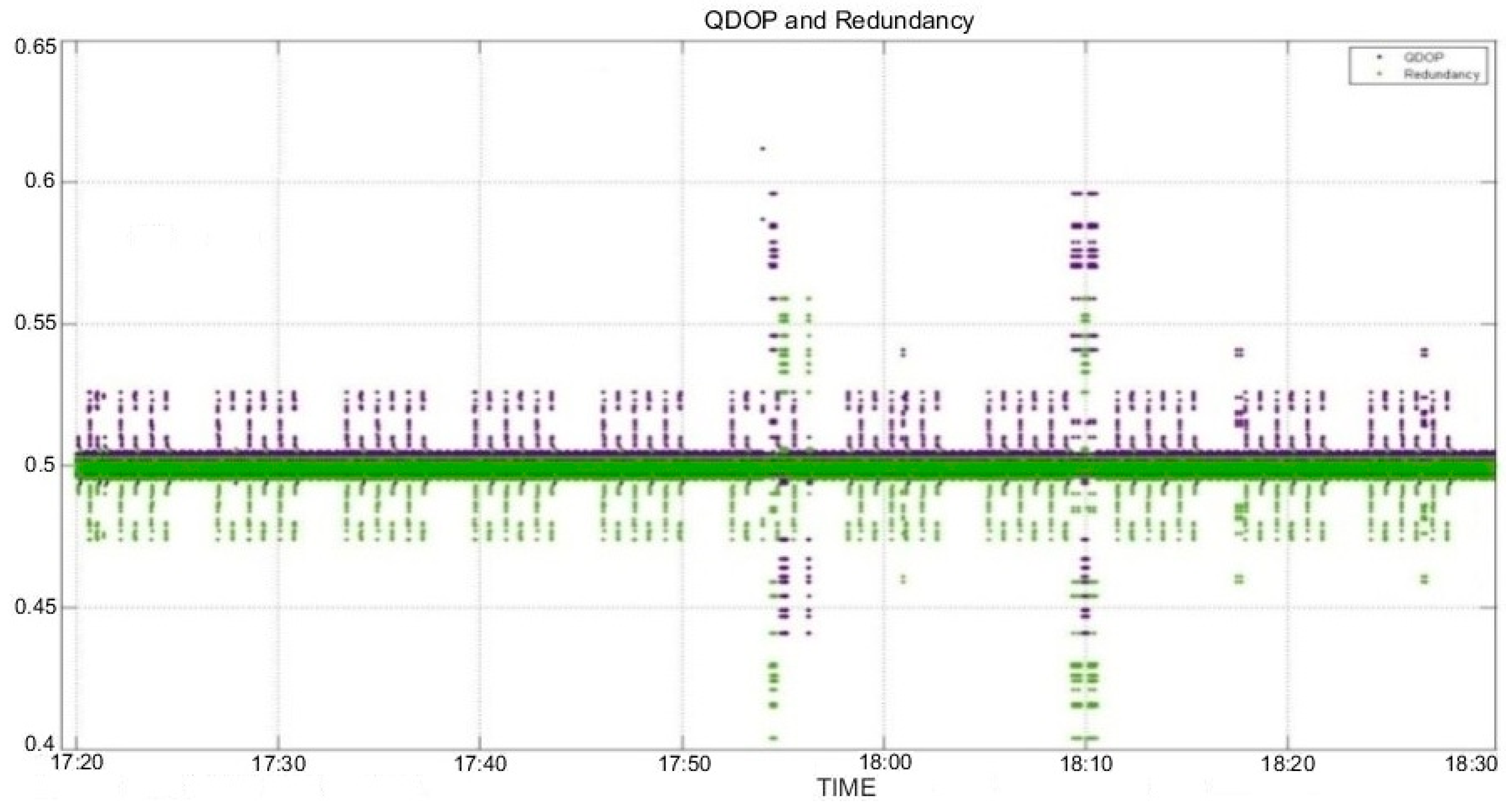
3.2.1. QDOP and Redundancy
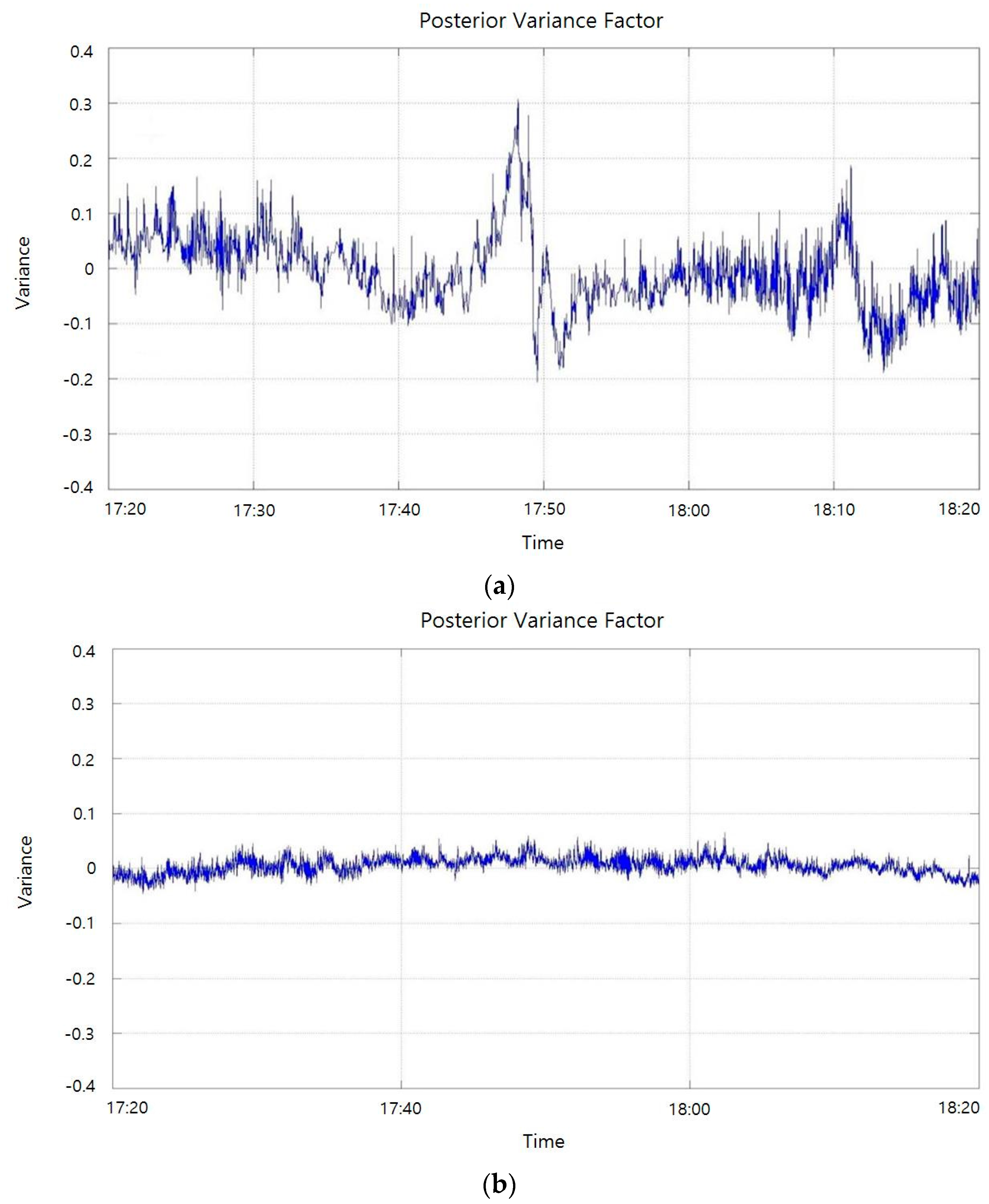
3.2.2. Analysis on Posterior Variance
3.2.3. Reliability
- -
- Internal reliability
- -
- External reliability
3.3. Improved Accuracy of GNSS Positioning Solution
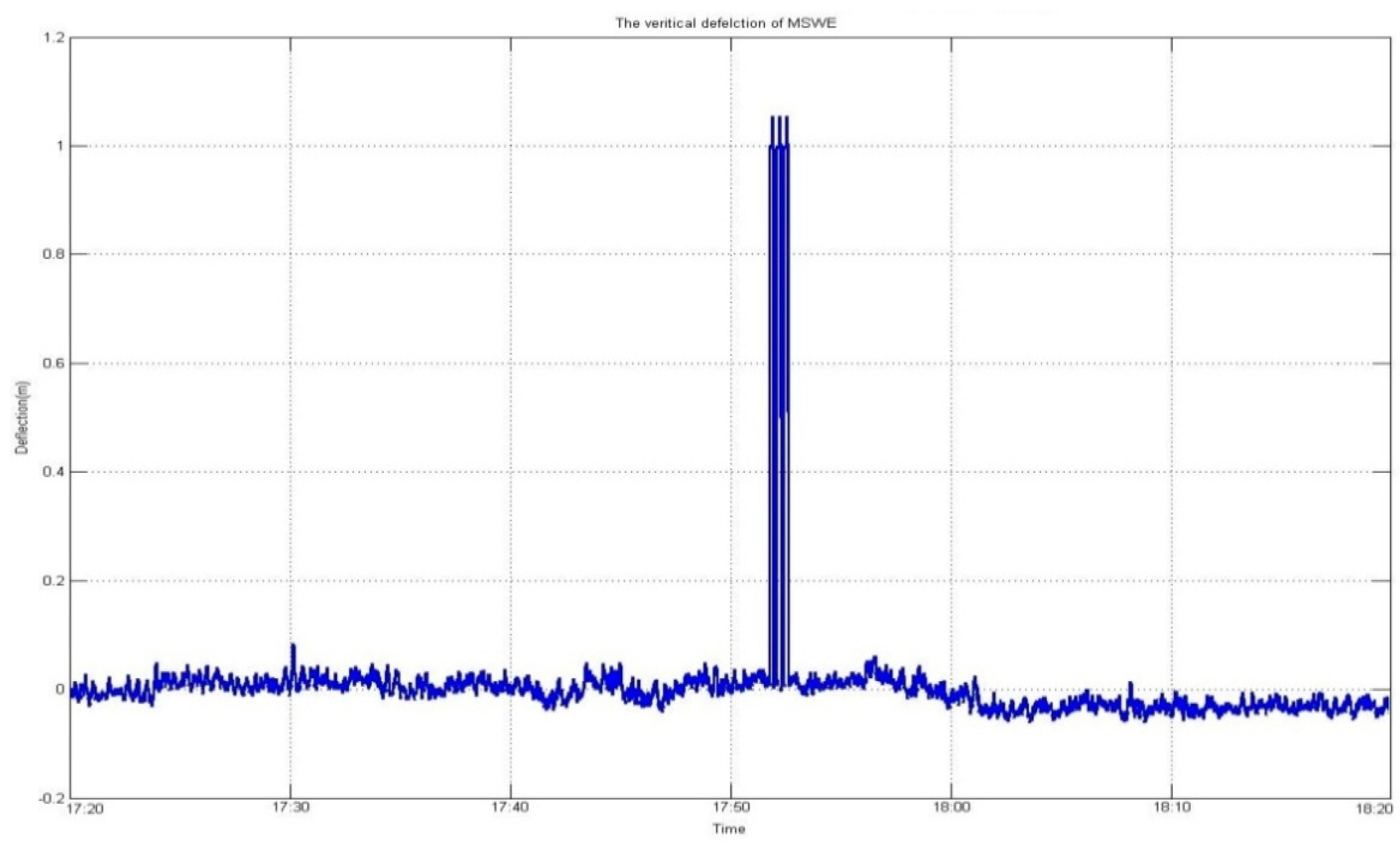
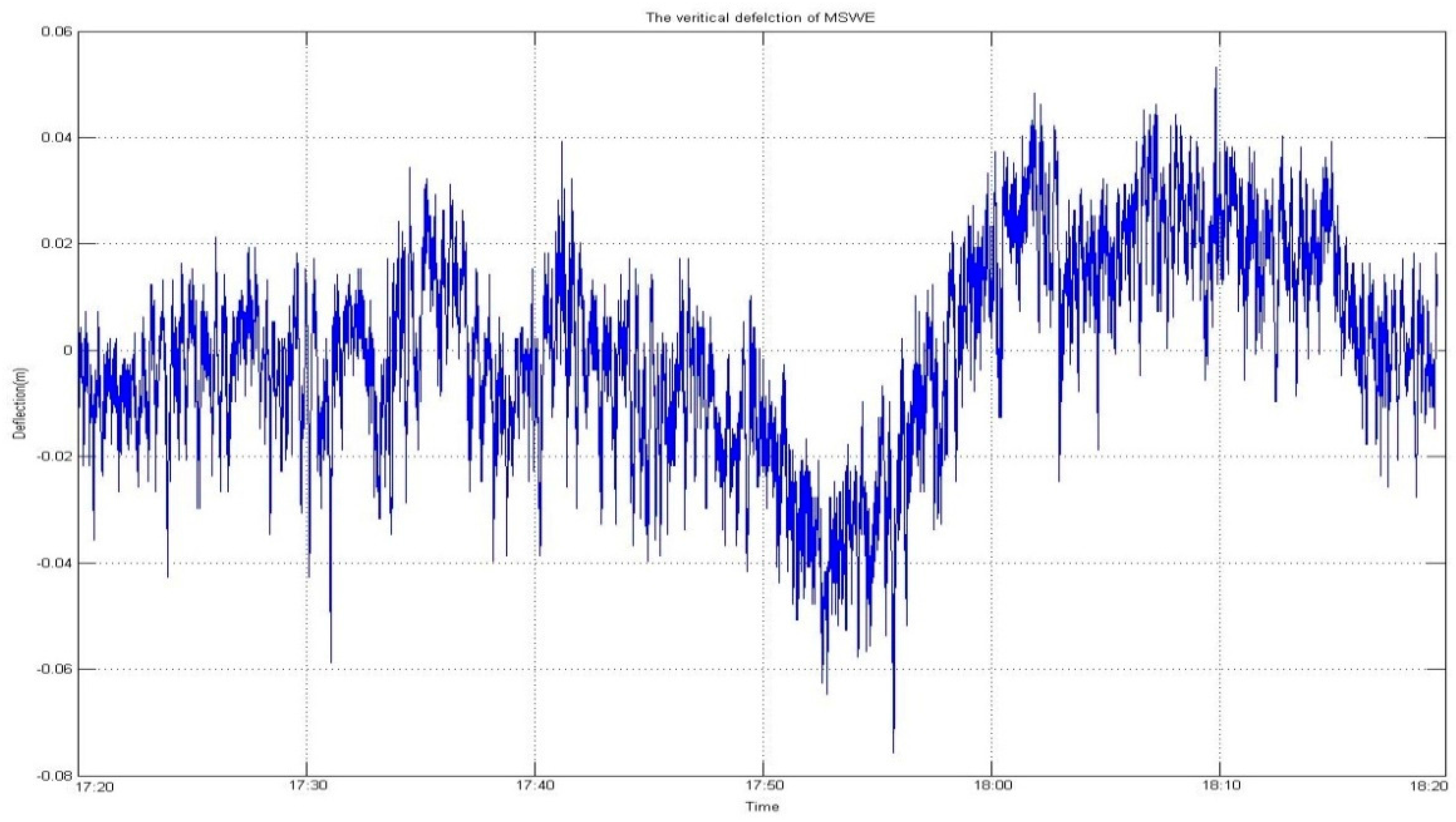
3.3.1. Enhanced Vertical Positioning
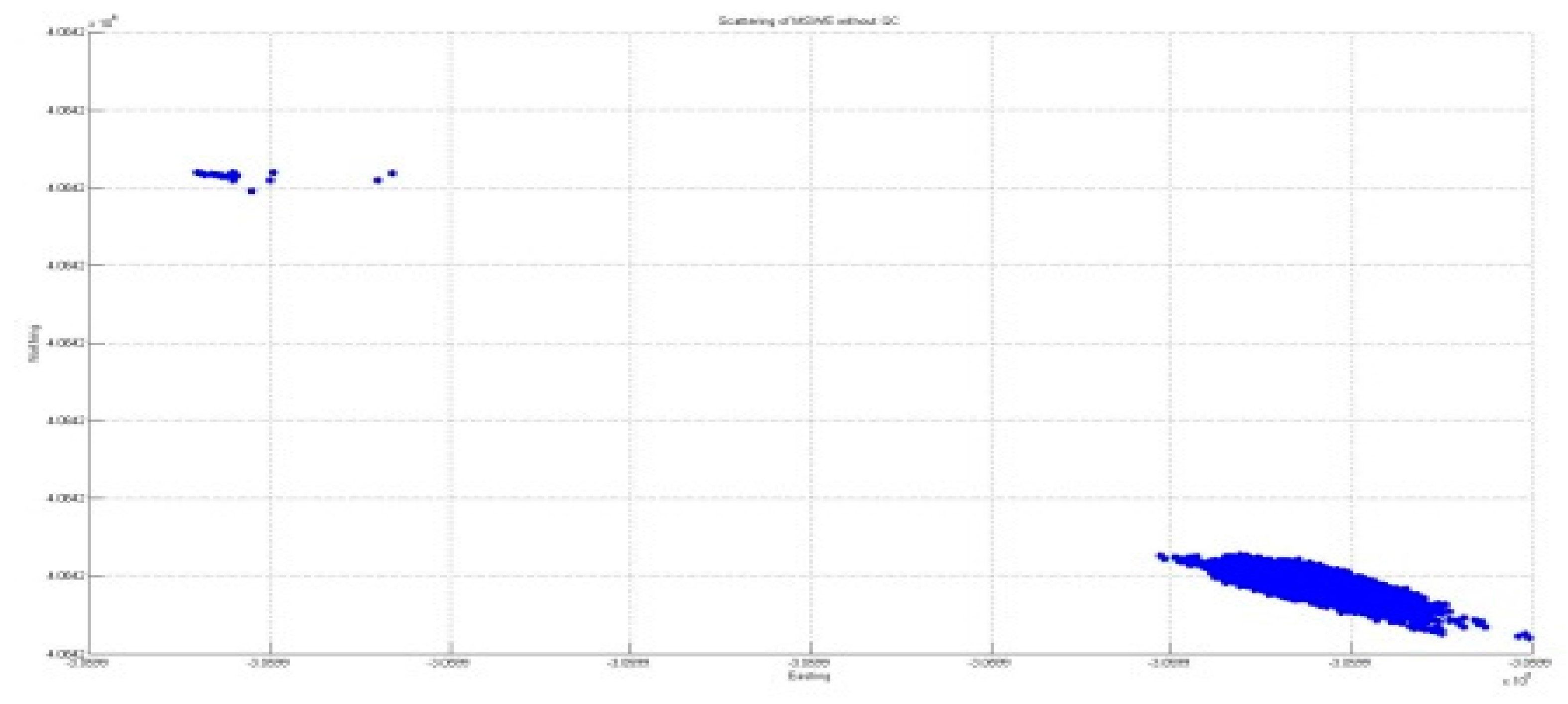
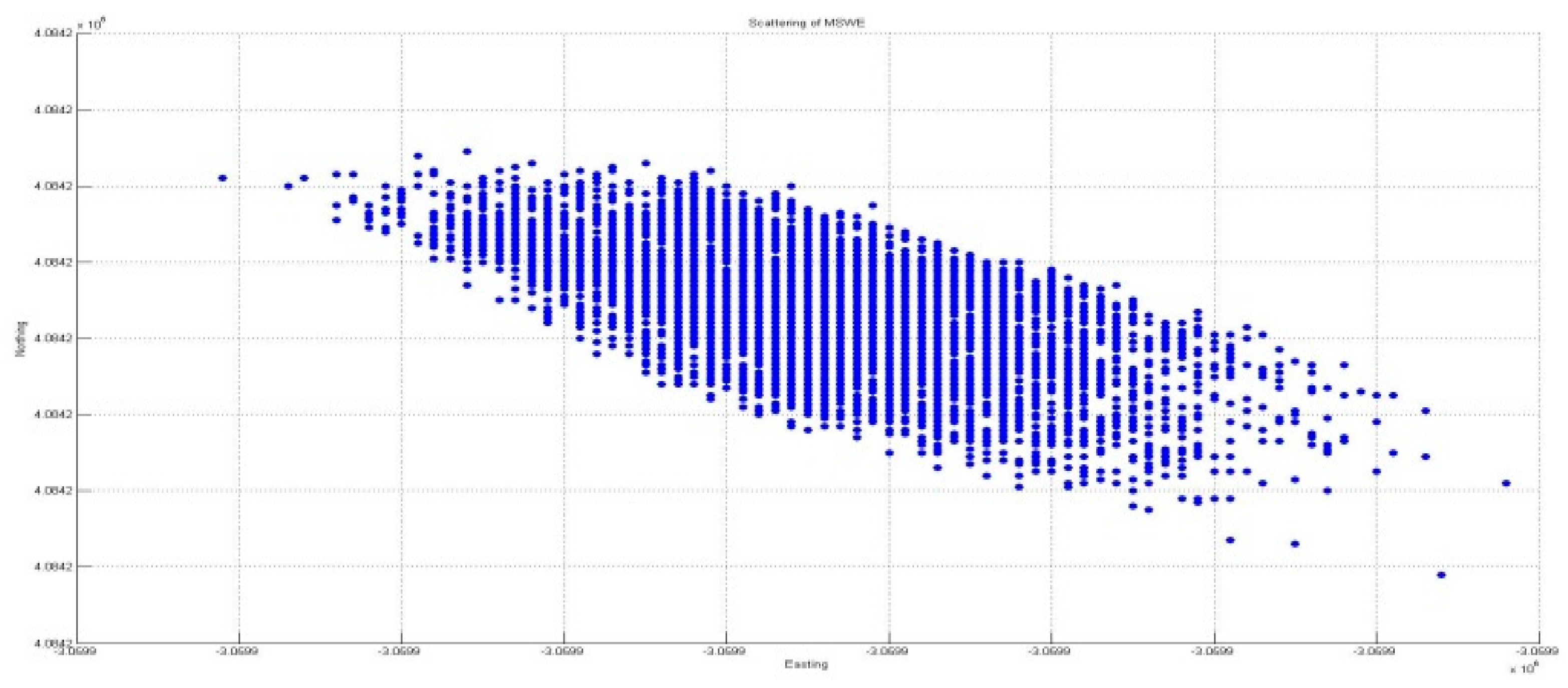
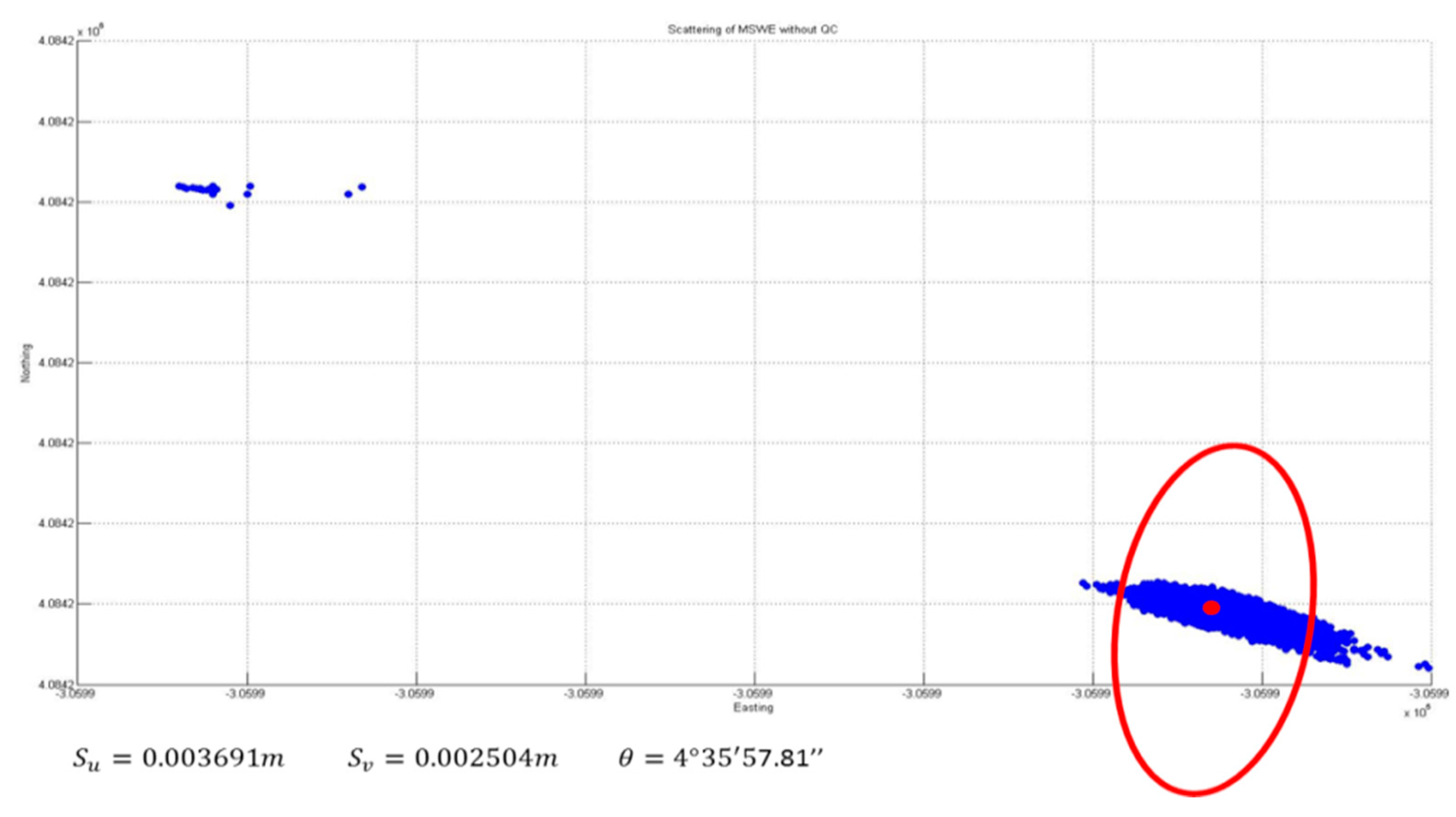
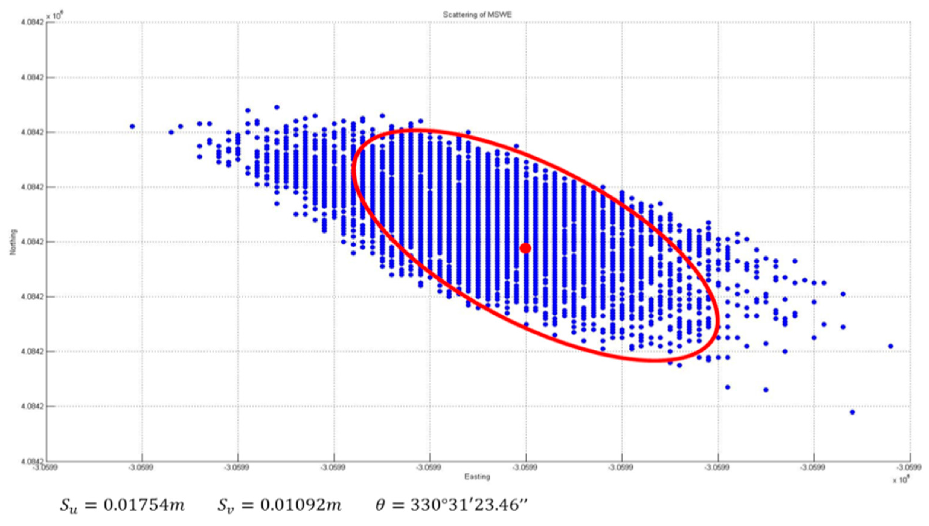
3.3.2. Horizontal Direction Positioning Solution
- -
- Error Ellipse Comparison
4. Concluding Remarks
Acknowledgments
Author Contributions
Conflicts of Interest
References
- Kuang, S.L. Optimization and Design of Deformation Monitoring Schemes. Ph.D. Thesis, University of New Brunswick, Fredericton, NB, Canada, 1991. [Google Scholar]
- Salzmann, M. MDB: A Design Tool for Integrated Navigation System. J. Geod. 1991, 65, 109–115. [Google Scholar]
- Teunissen, P.J.G.; Salzmann, M.A. A Recursive Slippage Test for Use in State-space Filtering. Manuscr. Geod. 1989, 14, 383–390. [Google Scholar]
- Baarda, W.W. A Testing Procedure for Use in Geodetic Network; Netherlands Geodetic Commission: Delft, The Netherlands, 1968. [Google Scholar]
- Förstner, W.; Gülch, E. A Fast Operator for Detection and Precise Location of Distinct Points, Corners and Centres of Circular Features. In Proceedings of the ISPRS Intercommission Workshop, Interlaken, Switzerland, 2–4 June 1987.
- Cross, P.A.; Hawksbee, D.J.; Nicolai, R. Quality measures for differential GPS positioning. Hydrogr. J. 1994, 72, 17–22. [Google Scholar]
- Lee, K.S. Application of Quality Control Procedure to Improve Reliability of GPS Positioning. Master’s Thesis, Changwon National University, Changwon, Korea, 2010. [Google Scholar]
- Park, J.C. A Study on SARX Models and Data Analysis Techniques for Structural Health Monitoring of a Cable-Supported Bridge. Ph.D. Thesis, Hanyang University, Seoul, Korea, 2009. [Google Scholar]
- Park, J.C.; Gil, H.B.; Kang, S.K.; Im, C.W. Dynamic Characteristics of a Cable-stayed Bridge Using Global Navigation Satellite System. J. KSCE 2010, 30, 375–382. [Google Scholar]
- Roberts, G.W.; Meng, X.; Dodson, A.H. The Use of Kinematic GPS and Triaxial Accelerometers to Monitor the Deflections of Large Bridges. In Proceedings of the 10th FIG Symposium on Deformation Measurements, Orange, CA, USA, 19–22 March 2001.


| Without QC | Applied QC | Improvement | |
|---|---|---|---|
| Max | 1.055 | 0.051 | 483% |
| Min | −0.062 | −0.076 | 122% |
| RMS | 0.088 | 0.018 | 489% |
| Without QC | With QC | ||
|---|---|---|---|
| Easting | Max | −3,059,909.6 | −3,059,886.35 |
| Min | −3,059,909.97 | −3,059,886.43 | |
| Northing | Max | 4,084,206.02 | 4,084,201.51 |
| Min | 4,084,205.42 | 4,084,201.4 | |
| RMS | 0.028 | 0.01 (280%) |
| Length of Major Axis | Azimuth | |
|---|---|---|
| Without QC | 0.0369 m | 4°35′57.81″ |
| Applied QC | 0.0375 m | 330°31′23.46″ |
| Difference | 47.52 mm | 34°4′13.95″ |
© 2016 by the authors; licensee MDPI, Basel, Switzerland. This article is an open access article distributed under the terms and conditions of the Creative Commons Attribution (CC-BY) license (http://creativecommons.org/licenses/by/4.0/).
Share and Cite
Lee, J.K.; Lee, J.O.; Kim, J.O. New Quality Control Algorithm Based on GNSS Sensing Data for a Bridge Health Monitoring System. Sensors 2016, 16, 774. https://0-doi-org.brum.beds.ac.uk/10.3390/s16060774
Lee JK, Lee JO, Kim JO. New Quality Control Algorithm Based on GNSS Sensing Data for a Bridge Health Monitoring System. Sensors. 2016; 16(6):774. https://0-doi-org.brum.beds.ac.uk/10.3390/s16060774
Chicago/Turabian StyleLee, Jae Kang, Jae One Lee, and Jung Ok Kim. 2016. "New Quality Control Algorithm Based on GNSS Sensing Data for a Bridge Health Monitoring System" Sensors 16, no. 6: 774. https://0-doi-org.brum.beds.ac.uk/10.3390/s16060774