Classification of Data from Electronic Nose Using Gradient Tree Boosting Algorithm


1
School of Electronic Science and Technology, Shenzhen University, Shenzhen 518060, China
2
Key Laboratory of Optoelectronic Devices and Systems of Ministry of Education and Guangdong Province, College of Optoelectronic Engineering, Shenzhen University, Shenzhen 518060, China
3
School of Information Engineering, Shenzhen University, Shenzhen 518060, China
*
Author to whom correspondence should be addressed.
Sensors 2017, 17(10), 2376; https://0-doi-org.brum.beds.ac.uk/10.3390/s17102376
Submission received: 16 August 2017
/
Revised: 2 October 2017
/
Accepted: 17 October 2017
/
Published: 18 October 2017
(This article belongs to the Special Issue Artificial Olfaction and Taste)
Abstract
:In this paper, an approach that can fast classify the data from the electronic nose is presented. In this approach the gradient tree boosting algorithm is used to classify the gas data and the experiment results show that the proposed gradient tree boosting algorithm achieved high performance on this classification problem, outperforming other algorithms as comparison. In addition, electronic nose we used only requires a few seconds of data after the gas reaction begins. Therefore, the proposed approach can realize a fast recognition of gas, as it does not need to wait for the gas reaction to reach steady state.
1. Introduction
An electronic nose, which imitates the perceptional mechanisms of biological olfactory organ, has been widely used in many applications such as the medical and diagnostic [1,2], food [3,4,5] and environment [6,7,8,9,10,11] monitor.
One important part of an electronic nose system is a pattern recognition system that would recognize the olfactory of the tested gas. Therefore, in the past decades, many pattern recognition algorithms have been introduced for the gas classification. In [12,13,14], a simple but quite effective method, the K-nearest neighbor (KNN) was first introduced in electronic nose applications for gas classification. The Gaussian mixture model (GMM) method [15,16] is also explored for the gas classification. Though Both KNN and GMM methods are simple, they suffer a limitation that their accuracy is limited when the size of train data is small. A binary decision tree (BDT) is first proposed in [17]. The BDT is easy understand and friendly to hardware implementation, but it is unstable and its accuracy is not high. In order to cope with nonlinearity of gas classification problem and to improve the classification accuracy, the advanced methods such as artificial neural networks (ANN) like multiple layer perception (MLP) [18,19,20], restricted boltzmann machines (RBM) [21,22], support vector machine (SVM) [23,24,25] and relevance vector machine(RVM) [26,27] are also presented. Despite the fact that these advanced methods [18,19,20,21,22,23,24,25,26,27] could provide the a high accuracy classification, a significant and practical disadvantage of these methods is that they can not directly handle the raw, time-sampled sensor response data due to the high dimensional patterns. In other words, a preprocessing block that extract the features from the raw data is necessary for the above mentioned advanced methods. Since featuring extracting is not straightforward and generally needs very complexity processing techniques, which will lead to the significantly increase of the power consumption and system complexity.
In order to overcome the limitations either on low accuracy or needing to extract features from raw data, in this paper, gradient tree boosting algorithm which could direct handle the raw, time-sampled sensor data is first introduced to the gas classification. Compared with conventional methods, the proposed methods have the following advantages [28]: (1) It can handle high-dimensional features without additional feature engineering; (2) Robust to overfitting; (3) Can naturally deal with the nonlinearity in the classification; (4) can provide high classification accuracy even with small size of train data.
Besides that, the proposed algorithm can realize the fast classification with high accuracy. Though there many techniques have been proposed to extract transient features [29,30,31,32] by performing certain operation on raw sampled data such as doing the exponential moving average or derivative to realize fast classification, no one have proposed to use the raw sampled data as transient features.
The rest of this article is organized as follows. In the next section, the proposed gradient tree boosting algorithm is presented. Section 3 discusses the experimental results that compare the performance of the classification accuracy of different classifier methods. Some concluding remarks are given in Section 4.
2. Gradient Tree Boosting Algorithm
Machine-learning techniques have been becoming more and more prevalent in many areas. Among the machine-learning algorithms, gradient tree boosting has shown huge success in many applications. On classification benchmarks gradient tree boosting achieved the leading results [33], ranging from ranking problems to rate prediction problem [34]. Since its invention [35], the recent development further advanced the advantage of the tree boosting algorithm. The Extreme Gradient Boosting, or called XGBoost [36], is a scalable tree boosting system. Due to several important optimizations in split finding and system design, XGBoost has achieved great success and been prevalently used in the winning teams in major data competitions like Kaggle and Knowledge Discovery and Data Mining cup (KDDCup) [36]. In the following of this chapter, the gradient tree boosting algorithm tailored for the gas classification is discussed.
2.1. Tree Ensemble and Learning Objective
Considering the given data set as , with representing the feature for data instance i (assuming ) and its target. Assume the number of data instances is n and the dimension of feature vector is m. For a tree ensemble model, the output is predicted by summing K additive functions:
where is the prediction given by the k-th classification and regression tree (CART) [37]. Figure 1 depicts the ensemble tree model.
Denote the number of leaves in a single CART as T, and define the structure of the tree that maps the data instance x to the corresponding leaf index as . Then in Equation (1), the prediction of k-th CART for i-th data instance can be written as
where w denote the leaf weights of the CART and represents the mapping function defined by the tree structure.
Then, the learning objective of the tree ensemble model can be set to minimize the following loss function:
where the differentiable convex loss function measures the difference the target and the prediction in Equation (1), and in the summation, n represents the number of data instances, K is the number of CARTs used in the algorithm. Here are the regularization terms for penalizing the model’s complexity and avoiding overfitting, defined by the number of leaves T and the square of leaf weights w:
where and are regularization parameters.
2.2. Gradient Boosting Algorithm
Here the goal of training the model is to minimize the overall loss function . However, traditional optimization methods cannot apply to minimize it in Euclidean space, since the loss function of the tree ensemble model in Equation (3) depends on each tree’s structure as well as parameters. To solve this problem and efficiently achieve this goal, the gradient tree boosting algorithm is proposed and developed [35,36,38]. In the following let us review the algorithm.
In training the model, at the -th iteration, define the loss function as
where represents the prediction of the ith instance at the th iteration. Then, to minimize it we additively add at t-th iteration, and the loss function becomes
In other words, we greedily add the tree which can most improves the model according to Equation (3). Therefore, at iteration t where we add the t-th CART, the objective is to find the tree structure of t-th CART that defines and , to minimize .
Firstly, note that by Taylor expansion, we can write the loss function as
with
representing the first and second order gradient statistics on respectively. At step t, the previous tree structures at are fixed and their loss function can be seen as constant, thus we can remove it and obtain the simplified learning objective at step t
Here represents the data instance set of leaf p, i.e., all the instances that are mapped to leaf leaf p.
Then, for a fixed tree structure , the optimal weight of leaf p is defined by the minimization equation
with defined by Equation (10), this function gives solution
Taking this optimal weight , the corresponding optimal loss function of Equation (10) becomes
Therefore, for each iteration t of constructing the t-th CART, our goal becomes finding its best tree structure q that gives the minimum .
However, in finding the best q, enumerating all possible tree structures is not practical. Instead, the greedy algorithm is used. Starting from a single leaf, we can iteratively split the tree nodes and add branches to the tree. For each iteration, denote the data instance set as I before splitting, and denote and respectively to be the instance sets of the left and right nodes after splitting. Because , using Equation (13), the loss function reduction after this splitting is given by
Therefore, to find the best tree structure, the algorithm iteratively adds the branches by choosing the splitting that maximizes .
3. Experimental Setup and Performance Evaluation
3.1. Experimental Setup and the Measurement Procedure
A block diagram of the automated gas delivery setup used to acquire the signatures of the target gases with the sensor array is shown in Figure 2. Eight commercial Figaro metal oxide semiconductor (MOS) sensors with diverse sensing performance are used to build the gas sensor array and their corresponding part numbers are listed in Table 1. As the working temperature of the sensor, which is controlled with a built-in heater and thus the voltage in sensor heater is also listed in Table 1. The electronic signal of these sensors are simultaneously acquired through chemical gas senor CGS-8 system in 10Hz sampling rate. Computer controlled mass flow controllers (MFCs) are used to control the flow rate of the target gas. Through changing the ratio of the flow rate between target gas and background gas, we can get a range of concentrations of target gas. For example, in the case that the background gas is air and the target gas is Methane . If we would like to set the target methane gas at concentration 100 ppm, we can first buy a bottle of methane with original concentration 500 ppm and then set the ratio of flow rate between air and methane to 4:1. Therefore, if we have a bottle of methane with concentration 500 ppm, any concentration between 0 to 500 ppm can be achieved by properly controlling the flow rate between air and methane through the MFCs. Before the gas reaction, the air is injected to the chamber for 500 s to clean the surface of gas sensors and get a stable baseline resistance. Then, thesensor array is exposed to the reaction gas for 160 s to ensure sensors reach the saturation status. In our case, six type gases, i.e., Carbon Monoxide , methoxymethane , Ethylene , Methane , Ethane and Hydrogen are used for the reaction. The concentration ranges for each target gas is from 20 ppm to 200 ppm with a stepsize 20 ppm. The reason why we chose these 6 gases is that they are the most common inflammable and explosive gases which may result in great damage when they leaked. The low and upper explosive levels for these gases are 12–74.2% VOL, 3.3–19% VOL, 2.7–36% VOL, 5–15% VOL, 3–12.4% VOL and 4.1–74.2% VOL, where 1% V is 10,000 ppm. And we think that realization the fast recognition of these 6 gases may help to prevent a conflagration in Petrochemical industry or in daily life.
3.2. Data Set and features
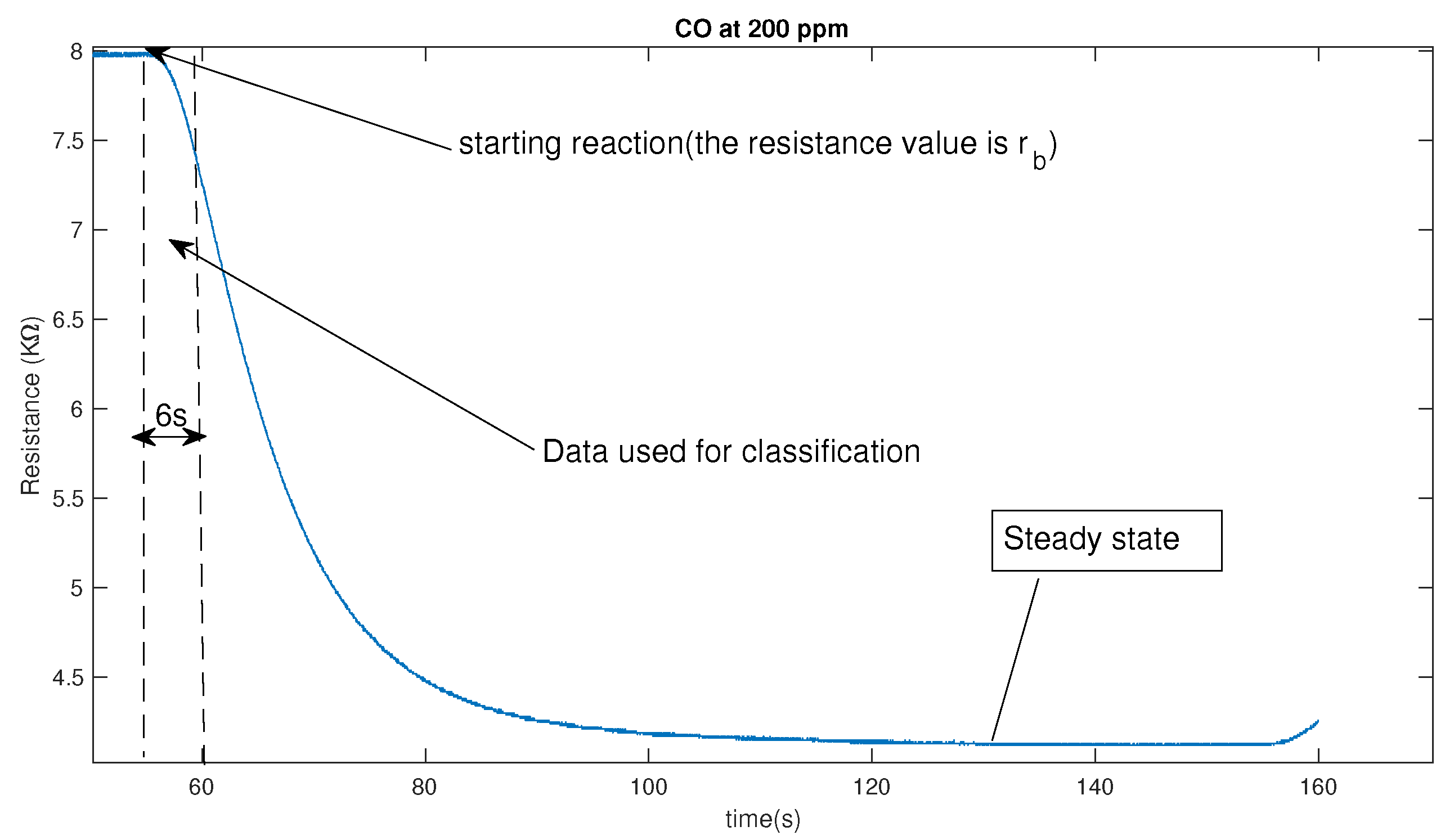
As there are 10 concentrations for each gas, for each type gas at each concentration, we make 25 repeated measurements and thus there are 250 measurements for each type gas. As there are 6 types in our case, totally we have samples in our data sets. It should be noted that the proposed algorithm can be directly applied to the raw data set and thus there is no need to do the preprocessing of the sampled raw data for the feature extraction. And, it is one advantage of the proposed algorithm, which can directly handle high-dimensional data without any feature extraction engineering. Besides that, we found that it only a small part of the time-sampled raw data is sufficient for the high-accuracy classification. In our case, we only use the first 6 s raw data since the reaction of the sensor started as shown in Figure 3. From the Figure 3 , at 200 ppm for gas , the gas sensor TGS2602 takes about 75 s to reach the steady state. Therefore, compared with existing method which use the sensor resistance at steady state as important features for the recognition, the proposed method can realize the recognition 12 time faster.
The first 6 s raw data (resistance value) of each sensor is directly used as features. As the sample rate of data acquisition device (DAQ) is 10 Hz, i.e., there are features of for i-th sensor at j-th measurement, which can be denoted as , where r represents the resistance value at certain time. In our E-nose, there are 8 gas sensors and thus there are features in total for j-th measurement, which can be denoted as . In order to reduce impact of the baseline drift, the final features vector the baseline resistance, denoted as , which is the resistance of gas sensor before starting reaction is subtracted from feature vector, i.e., the final feature vector can be expressed as .
3.3. Results
For each type gas, the dataset consisted of 250 samples is randomly split into training and test sets. We used the same training gas sets to train the different classification algorithms, including the proposed one. And the test set is also the same between the proposed algorithm and the comparison algorithms. In other words, all the algorithms are learned from same data and test their classification accuracy on the same data. Therefore, under this circumstance, the algorithm with highest classification accuracy should be best one. Classification accuracy is one of the most important evaluation metrics for supervised learning algorithms and it can be obtained by the number of correctly recognized examples is divided by the total number of testing examples. Moreover, in order to do a fair comparison with the GMM, KNN, MLP, and SVM methods, the same condition (the same raw sampled data) is also applied to these methods, though generally some preprocessing techniques such as Principal Component Analysis (PCA), fast fourier transform (FFT) and discrete wavelet transform (DWT) should be applied to raw data to extract features when the GMM, KNN, MLP, and SVM methods are used. In addition, as the training set and test set are randomly selected from the whole dataset, to eliminate the bias of the test result, we repeated this train-test procedure 100 times with different random splits. Then we average the accuracy of each test to get the accuracy for each classifier.
Table 2 shows the classification performance for various algorithms. It can be seen from Table 2, the GMM reach the lowest accuracy. In the GMM model, it assumes that the probability distribution of observations in the overall population can be represented by mixture Gaussian distribution, but this assumption is not always satisfied. Moreover, estimating the covariance matrices for the Gaussian components becomes difficult when the feature space gets large and is comparable to the number of the data points. Therefore, in our case where the dimension of feature space can get as large as 480, the classification performance of GMM is significantly poor. Table 2 also shows that the proposed gradient tree boosting achieves the highest classification accuracy. It verifies the claim that the proposed gradient tree boost algorithm can handle high-dimensional features without additional feature engineering and still achieve high accuracy while the existing methods such as GMM, KNN and SVM can not. Without any additional feature engineering, the raw sampled data can be directed taken as the input of the proposed gradient tree boost method, which could lead to the fast recognition of the gas.
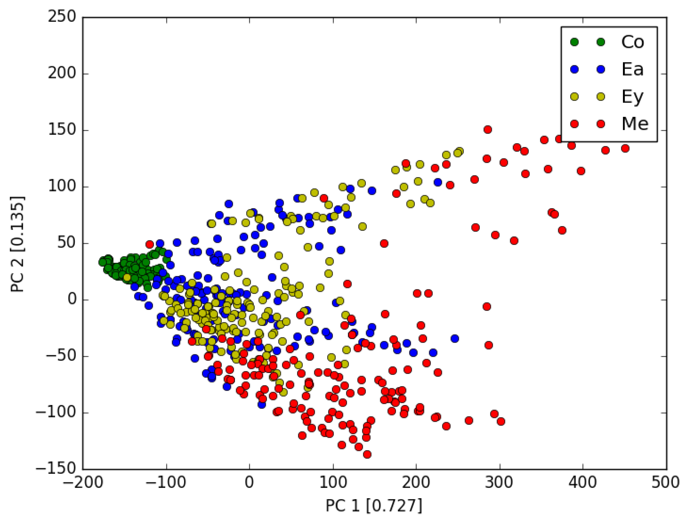
Here to make the analysis more complete, we also tested the following approach. We first use the PCA to reduce the dimension of feature space from 360 to 10, with the total explain variance ratio >0.995. Then test each algorithm with the PCA features. The performances are listed in Table 3. We found that for each algorithm, PCA processing does not improve the accuracy (We also tested other different numbers of PCA components, the results are similar.). The Figure 4 shows the first 2 most dominant components (with explain variance ratio of 0.727 and 0.135 respectively) for 4 gases. The reason why PCA cannot significantly improve the accuracy can be seen from Figure 4 . We can see that different gases have different properties, but the boundary of each gas is not clear define. In other words, for the existing algorithm such as KNN, GMM, MLP and SVM, more sophisticated feature extracting engineering is required to further improve the accuracy. Moreover, though the PCA processing reduces the feature dimension, it eliminates certain useful information when removing the noise.
3.4. An Example of Application Based on Raw Data to Realize Fast Recognition
Although natural gas (mainly consist of Methane ) is environmental friendly, it can lead to a serious damage if they leak. It is stored in pressurized steel cylinders in liquid form and vaporize at normal temperatures. When it leaks and reach certain concentration, ignition may happen and cause an explosion. Therefore, the detection of Methane leakage as early as possible is quite desirable. In order to test whether the proposed algorithm based on raw sampled data can realize the fast detection the Methane leakage on real application in a open environment, we lift the glass cover of the gas chamber so the sensor array can exposed to real environment. Then, we turn on the valve of methane bottle and let methane gas leak through a rubber pipe which is placed near the sensor array. The leakage only last for 6 s and the 6 s raw sampled data collected by the sensor system is direct fed into the proposed gradient tree boost classifier which will recognize whether the methane is existed or not. Such measurements are repeated for 40 times, and the proposed gradient tree boost classifier recognizes the sample correctly as methane 39 times, while GMM, KNN, MLP and SVM classifiers only reach 13, 31, 28, 34 times. In other words, even in an open environment, the proposed gradient tree boost classifier can realize fast detection of methane leakage with high accuracy, which may help to prevent a fire cased by natural gas leakage.
4. Conclusions
In this paper, we applied Gradient tree boosting algorithm to solve the multi-classification problems for 6 different gases. We showed that this algorithm achieved higher performance than that of conventional algorithms. Besides, since the approach we used only need to take the first few seconds data of the electronic nose after gas reaction, without any additional feature engineering, it is able to detect certain gas quickly and efficiently. Therefore, our approach could have great potential in practical application.
Acknowledgments
This work was supported by the National Natural Science Foundation of China (Grant NO. 61601301, 61504086), the Fundamental Research Foundation of Shenzhen (Grant NO. JCYJ20160308094919279, JCYJ20170302151123005, JCYJ20150626090521275), the key Project department of Education of Guangdong Province (No. 2015KQNCX142) and the Natural Science Foundation of SZU (Grant NO. 2016020).
Author Contributions
The work presented in this paper is a collaborative development by all of the authors. Wenbin Ye and Yuan Luo contributed to the idea of the incentive mechanism and designed the algorithms. Xiaojin Zhao, Xiaofang Pan and Yuan Cao were responsible for some parts of the theoretical analysis and the paper check. All of the authors were involved in writing the paper.
Conflicts of Interest
The authors declare no conflict of interest.
References
- D’Amico, A.; Di Natale, C.; Paolesse, R.; Macagnano, A.; Martinelli, E.; Pennazza, G.; Santonico, M.; Bernabei, M.; Roscioni, C. Olfactory systems for medical applications. Sens. Actuators B Chem. 2008, 1, 458–465. [Google Scholar] [CrossRef]
- Kiani, S.; Minaei, S.; Ghasemi-Varnamkhasti, M. Application of electronic nose systems for assessing quality of medicinal and aromatic plant products: A review. J. Appl. Res. Med. Aromat. Plants 2016, 3, 1–9. [Google Scholar] [CrossRef]
- Peris, M.; Escuder-Gilabert, L. The electronic nose applied to dairy products: A review. Sens. Actuators B Chem. 2009, 638, 1–15. [Google Scholar]
- Loutfi, A.; Coradeschi, S.; Mani, G.K.; Shankar, P.; Rayappan, J.B.B. Electronic noses for food quality: A review. J. Food Eng. 2015, 144, 103–111. [Google Scholar] [CrossRef]
- Baietto, M.; Wilson, A.D. Electronic-nose applications for fruit identification, ripeness and quality grading. Sensors 2015, 15, 899–931. [Google Scholar] [CrossRef] [PubMed]
- RajamÄki, T.; Arnold, M.; Venelampi, O.; Vikman, M.; RÄsÄnen, J.; ItÄvaara, M. An electronic nose and indicator volatiles for monitoring of the composting process. Water Air Soil Pollut. 2005, 162, 71–87. [Google Scholar]
- Romain, A.C.; Nicolas, J. Long term stability of metal oxide-based gas sensors for e-nose environmental applications: An overview. Sens. Actuators B Chem. 2010, 146, 502–506. [Google Scholar] [CrossRef]
- Brudzewski, K.; Osowski, S.; Pawlowski, W. Metal oxide sensor arrays for detection of explosives at sub-parts-per million concentration levels by the differential electronic nose. Sens. Actuators B Chem. 2012, 161, 528–533. [Google Scholar] [CrossRef]
- Capelli, L.; Dentoni, L.; Sironi, S.; Del Rosso, R. The need for electronic noses for environmental odour exposure assessment. Water Sci. Technol. 2014, 69, 135–141. [Google Scholar] [CrossRef] [PubMed]
- Capelli, L.; Sironi, S.; Del Rosso, R. Electronic noses for environmental monitoring applications. Sensors 2014, 14, 19979–20007. [Google Scholar] [CrossRef] [PubMed] [Green Version]
- Deshmukh, S.; Bandyopadhyay, R.; Bhattacharyya, N.; Pandey, R.A.; Jana, A. Application of electronic nose for industrial odors and gaseous emissions measurement and monitoring—An overview. Talanta 2015, 144, 329–340. [Google Scholar] [CrossRef] [PubMed]
- Gutierrez-Osuna, R.; Gutierrez-Galvez, A.; Powar, N. Transient response analysis for temperature-modulated chemoresistors. Sens. Actuators B Chem. 2003, 93, 57–66. [Google Scholar] [CrossRef]
- Gebicki, J.; Szulczynski, B.; Kaminski, M. Determination of authenticity of brand perfume using electronic nose prototypes. Meas. Sci. Technol. 2015, 26, 125103. [Google Scholar] [CrossRef]
- Yang, J.; Sun, Z.; Chen, Y. Fault detection using the clustering-kNN rule for gas sensor arrays. Sensors 2016, 16, 2069. [Google Scholar] [CrossRef] [PubMed]
- Belhouari, S.B.; Bermak, A.; Shi, M.; Chan, P.C. Fast and robust gas identification system using an integrated gas sensor technology and Gaussian mixture models. IEEE Sens. J. 2005, 5, 1433–1444. [Google Scholar] [CrossRef]
- Leidinger, M.; Reimringer, W.; Alepee, C.; Rieger, M.; Sauerwald, T.; Conrad, T.; Schuetze, A. Gas measurement system for indoor air quality monitoring using an integrated pre-concentrator gas sensor system. In Proceedings of the Micro-Nano-Integration, GMM-Workshop, Duisburg, Germany, 5–6 October 2016; pp. 1–6. [Google Scholar]
- Hassan, M.; Bermak, A. Gas classification using binary decision tree classifier. In Proceedings of the 2014 IEEE International Symposium on Circuits and Systems (ISCAS), Melbourne, VIC, Australia, 1–5 June 2014; pp. 2579–2582. [Google Scholar]
- Brezmes, J.; Ferreras, B.; Llobet, E.; Vilanova, X.; Correig, X. Neural network based electronic nose for the classification of aromatic species. Anal. Chim. Acta 1997, 348, 503–509. [Google Scholar] [CrossRef]
- Zhai, X.; Ali, A.A.S.; Amira, A.; Bensaali, F. MLP neural network based gas classification system on Zynq SoC. IEEE Access 2016, 4, 8138–8146. [Google Scholar] [CrossRef]
- Omatul, S.; Yano, M. Mixed Odors Classification by Neural Networks. In Proceedings of the 2015 IEEE 8th International Conference on Intelligent Data Acquisition and Advanced Computing Systems: Technology and Applications (IDAACS), Warsaw, Poland, 24–26 September 2015; pp. 171–176. [Google Scholar]
- Langkvist, M.; Loutfi, A. Unsupervised feature learning for electronic nose data applied to Bacteria Identification in Blood. In Proceedings of the NIPS 2011 Workshop on Deep Learning and Unsupervised Feature Learning, Granada, Spain, 12–17 December 2011; pp. 1–7. [Google Scholar]
- Liu, Q.; Hu, X.; Ye, M.; Cheng, X.; Li, F. Gas recognition under sensor drift by using deep learning. Int. J. Intell. Syst. 2015, 30, 907–922. [Google Scholar] [CrossRef]
- Pardo, M.; Sberveglieri, G. Classification of electronic nose data with support vector machines. Sens. Actuators B Chem. 2005, 107, 730–737. [Google Scholar] [CrossRef]
- Acevedo, F.; Maldonado, S.; Dominguez, E.; Narvaez, A.; Lopez, F. Probabilistic support vector machines for multi-class alcohol identification. Sens. Actuators B Chem. 2007, 122, 227–235. [Google Scholar] [CrossRef]
- Lentka, Ł.; Smulko, J.M.; Ionescu, R.; Granqvist, C.G.; Kish, L.B. Determination of gas mixture components using fluctuation enhanced sensing and the LS-SVM regression algorithm. Metrol. Meas. Syst. 2015, 3, 341–350. [Google Scholar] [CrossRef]
- Wang, X.; Ye, M.; Duanmua, C. Classification of data from electronic nose using relevance vector machines. Sens. Actuators B Chem. 2009, 140, 143–148. [Google Scholar] [CrossRef]
- Wang, T.; Cai, L.; Fu, Y.; Zhu, T. A wavelet-based robust relevance vector machine based on sensor data scheduling control for modeling mine gas gushing forecasting on virtual environment. Math. Probl. Eng. 2013, 2013. [Google Scholar] [CrossRef]
- Krauss, C.; Do, X.A.; Huck, N. Deep neural networks, gradient-boosted trees, random forests: Statistical arbitrage on the S&P 500. Eur. J. Oper. Res. 2017, 2, 689–702. [Google Scholar]
- Muezzinoglu, M.K.; Vergara, A.; Huerta, R.; Rulkov, N.; Rabinovich, M.; Selverston, A.; Abarbanel, H. Acceleration of chemo-sensory information processing using transient features. Sens. Actuators B Chem. 2009, 137, 507–512. [Google Scholar] [CrossRef]
- Siadat, M.; Sambemana, H.; Lumbreras, M. New transient feature for metal oxide gas sensor response processing. Procedia Eng. 2012, 47, 52–55. [Google Scholar] [CrossRef]
- Siadat, M.; Losson, E.; Ahmadou, D.; Lumbreras, M. Detection optimization using a transient feature from a metal oxide gas sensor array. Sens. Transducers 2014, 27, 340–341. [Google Scholar]
- Yan, J.; Guo, X.; Duan, S.; Jia, P.; Wang, L.; Peng, C.; Zhang, S. Electronic Nose Feature Extraction Methods: A Review. Sensors 2015, 15, 27804–27831. [Google Scholar] [CrossRef] [PubMed]
- Li, P. Robust LogitBoost and Adaptive Base Class (ABC) LogitBoost. Available online: https://arxiv.org/ftp/arxiv/papers/1203/1203.3491.pdf (accessed on 13 August 2017).
- He, X.; Pan, J.; Jin, O.; Xu, T.; Liu, B.; Xu, T.; Shi, Y.; Atallah, A.; Herbrich, R.; Bowers, S.; et al. Practical Lessons from Predicting Clicks on Ads at Facebook. In Proceedings of the Eighth International Workshop on Data Mining for Online Advertising, New York, NY, USA, 24–27 August 2014; pp. 51–59. [Google Scholar]
- Friedman, J.H. Greedy function approximation: A gradient boosting machine. Ann. Stat. 2001, 29, 1189–1232. [Google Scholar] [CrossRef]
- Chen, T.; Guestrin, C. Xgboost: A scalable tree boosting system. In Proceedings of the 22nd ACM SIGKDD International Conference on Knowledge Discovery and Data Mining, San Francisco, CA, USA, 13–17 August 2016; pp. 785–794. [Google Scholar]
- Breiman, L.; Friedman, J.; Stone, C.J.; Olshen, R.A. Classification and Regression Trees; CRC Press: Boca Raton, FL, USA, 1984. [Google Scholar]
- Friedman, J.; Hastie, T.; Tibshirani, R. Additive logistic regression: A statistical view of boosting (with discussion and a rejoinder by the authors). Ann. Stat. 2000, 28, 337–407. [Google Scholar] [CrossRef]
Figure 1.
Tree Ensemble Model. The final prediction for an instance is the sum of predictions from each tree.
Figure 1.
Tree Ensemble Model. The final prediction for an instance is the sum of predictions from each tree.

Figure 2.
Experimental setup to acquire signatures of the target gases with the sensor array.

Figure 3.
The response of a metal-oxide based chemical sensor to 200 ppm of .

Figure 4.
2-dimensional PCA plot of 4 gases.


Table 1.
Types of metal oxide semiconductor (MOS) sensors (provided by Figaro Inc.)
| Channel | Sensor Part Number | Voltage in Sensor Heater |
|---|---|---|
| 0 | TGS821 | 5 V |
| 1 | TGS812 | 5 V |
| 2 | TGS2610 | 5 V |
| 3 | TGS2612 | 5 V |
| 4 | TGS3870 | 5 V |
| 5 | TGS2611 | 5 V |
| 6 | TGS816 | 5 V |
| 7 | TGS2602 | 5 V |
© 2017 by the authors. Licensee MDPI, Basel, Switzerland. This article is an open access article distributed under the terms and conditions of the Creative Commons Attribution (CC BY) license (http://creativecommons.org/licenses/by/4.0/).
Share and Cite
MDPI and ACS Style
Luo, Y.; Ye, W.; Zhao, X.; Pan, X.; Cao, Y. Classification of Data from Electronic Nose Using Gradient Tree Boosting Algorithm. Sensors 2017, 17, 2376. https://0-doi-org.brum.beds.ac.uk/10.3390/s17102376
AMA Style
Luo Y, Ye W, Zhao X, Pan X, Cao Y. Classification of Data from Electronic Nose Using Gradient Tree Boosting Algorithm. Sensors. 2017; 17(10):2376. https://0-doi-org.brum.beds.ac.uk/10.3390/s17102376
Chicago/Turabian StyleLuo, Yuan, Wenbin Ye, Xiaojin Zhao, Xiaofang Pan, and Yuan Cao. 2017. "Classification of Data from Electronic Nose Using Gradient Tree Boosting Algorithm" Sensors 17, no. 10: 2376. https://0-doi-org.brum.beds.ac.uk/10.3390/s17102376
Note that from the first issue of 2016, this journal uses article numbers instead of page numbers. See further details here.