A Modified Empirical Wavelet Transform for Acoustic Emission Signal Decomposition in Structural Health Monitoring

1
School of Automation Science and Electrical Engineering, Beihang University, Beijing 100191, China
2
Collaborative Innovation Center of Advanced Aero-Engine, Beihang University, Beijing 100191, China
*
Author to whom correspondence should be addressed.
Sensors 2018, 18(5), 1645; https://0-doi-org.brum.beds.ac.uk/10.3390/s18051645
Submission received: 14 April 2018
/
Revised: 13 May 2018
/
Accepted: 18 May 2018
/
Published: 21 May 2018
(This article belongs to the Special Issue Mechatronic Systems for Automatic Vehicles)
Abstract
:The acoustic emission (AE) method is useful for structural health monitoring (SHM) of composite structures due to its high sensitivity and real-time capability. The main challenge, however, is how to classify the AE data into different failure mechanisms because the detected signals are affected by various factors. Empirical wavelet transform (EWT) is a solution for analyzing the multi-component signals and has been used to process the AE data. In order to solve the spectrum separation problem of the AE signals, this paper proposes a novel modified separation method based on local window maxima (LWM) algorithm. It searches the local maxima of the Fourier spectrum in a proper window, and automatically determines the boundaries of spectrum segmentations, which helps to eliminate the impact of noise interference or frequency dispersion in the detected signal and obtain the meaningful empirical modes that are more related to the damage characteristics. Additionally, both simulation signal and AE signal from the composite structures are used to verify the effectiveness of the proposed method. Finally, the experimental results indicate that the proposed method performs better than the original EWT method in identifying different damage mechanisms of composite structures.
1. Introduction
Composite materials are widely used in aircraft structures because of their advantages of stiffness, strength, light weight and excellent fatigue and corrosion resistance [1,2,3]. However, the various damage mechanisms of composite structures are very difficult to predict. Structural health monitoring (SHM), which can assess the structure status in real time and supply an early warning, has been proposed to confront this challenge [4,5]. Acoustic emission (AE) is an attractive technique for SHM which is sensitive, can detect various types of composite material damage and needs only a small number of sensors [3,6,7]. The exact health state can be obtained by monitoring the AE signals. Furthermore, damage information such as damage mechanisms, damage position and residual life could also be extracted when the AE signals can be accurately collected and analyzed [8]. At present, both traditional AE characteristic parameters and new signal processing methods can be used to analyze AE signals.
When composite structures are exposed to an external load, AE signals will occur from matrix cracking, matrix/fiber debonding, delamination, and fiber fracture [9]. Following the theory of plate wave, the generated waves will propagate in all directions, and form different modes. The difference of these modes is due to the particle displacement: in the plane (IP) for the symmetric or extensional mode and outside to the plane (OP) for the antisymmetric or flexural mode [10]. For the extensional mode, all frequency components travel at the same velocity, but for the flexural mode, the high frequency components travel faster than the low frequency components [11]. In practical structures, the signals detected by AE sensors depend on various factors, such as the structures’ properties (including the material, width, geometry, and so on), damage source orientation, damage location, signal attenuation, wave dispersion, boundary reflections and other interference phenomenon. Therefore, all these factors have to be taken into account during the AE data analysis [10].
A major issue is how to distinguish between the different damage mechanisms according to the characteristics of the AE signal. Many studies have used time features, frequency characteristics, or time-frequency methods to identify the damage mechanisms [10,11,12,13,14], but they were only applied in simple laboratory experiments. For complex structures, Sause and Hamstad established an effective finite element modeling (FEM) routine to interpret the AE signal behavior [15,16,17,18,19,20], which can give advice about how to extend the laboratory results to a practical scenario. In order to assess the real-time damage mechanisms, Martínez-Jequier et al. [21] designed appropriate hardware frequency filters to split the extensional and flexural modes of the damage AE signals; Yaacoubi and Dahmene [22] thought about the large data sets of the collected data during the composite SHM, and explored various innovative processing techniques to save computing time. Additionally, based on the variety of signal processing methods, a large number of studies have correlated specific AE signal features with the progression of damage. Gutkin et al. [23] identified some damage mechanisms of CFRP through pattern recognition algorithm based on five representative AE parameters (peak amplitude, peak frequency, energy, rise time and duration). McCrory et al. [24] classified the damage of matrix and delamination of CFRP based on AE signals through three classification techniques. Kumar et al. [25] considered significant AE parameters, such as counts, energy, signal strength, absolute energy and hits, and used an artificial neural network to predict the failure strength of composite laminates. Beheshtizaeh and Mostafapour [26] indicated that wavelet analysis was suitable to process the AE signals in three-point bending load of composites structure, but the proper wavelet type should be selected.
Recently, inspired by wavelet transform and empirical mode decomposition (EMD) [27], the empirical wavelet transform (EWT) has been developed by Gilles [28,29]. Amezquita-Sánchez et al. [30] employed EWT to estimate both natural frequencies and damping ratios of large civil structures. Yuan and Sadhu [31] used EWT to separate the closely-spaced natural frequencies of structures. The main idea of EWT is to determine the Fourier segments and then design a series of wavelet filters to decompose the signal into several sub-signals. EWT became adaptive when the Fourier segments were automatically determined. The empirical rule was to find all the local maxima of the spectrum and then use the center of the two adjacent local maxima as the boundaries of Fourier segments [32]. Some researchers have proposed solutions to modify the Fourier segments. Zheng et al. [33] proposed a method of adaptive parameterless EWT to fulfill an adaptive separation of the Fourier spectrum. Wang et al. [34] developed the sparsity-guided EWT to automatically establish Fourier segments. Song et al. [35] employed the scale-space histogram segmentation to determine the boundaries adaptively. However, for damage AE signals, when strong noise or frequency dispersion exist in the Fourier spectrum of the signals, such Fourier segmentation solutions are not always reliable and useful.
In this paper, local window maxima (LWM) algorithm is proposed to automatically determine the boundaries of Fourier segments, and it is appropriate for EWT to analyze the damage AE signals of composite structures. The key ideas of the algorithm are to search all the local maxima of the Fourier spectrum in an optimal window and then to obtain the segmentation boundaries. Since different damage mechanisms for composite structures have different frequency ranges, separating the different damage mechanisms is equivalent to decomposing the AE signals in the Fourier spectrum. The analysis results on a simulation signal show that this method can effectively obtain the peak frequency bands. In addition, the pencil-lead breaks (PLB) and three-point bending experiments on the composite structure is carried out to prove the applicability of the proposed solution.
2. The Modified Empirical Wavelet Transform Method
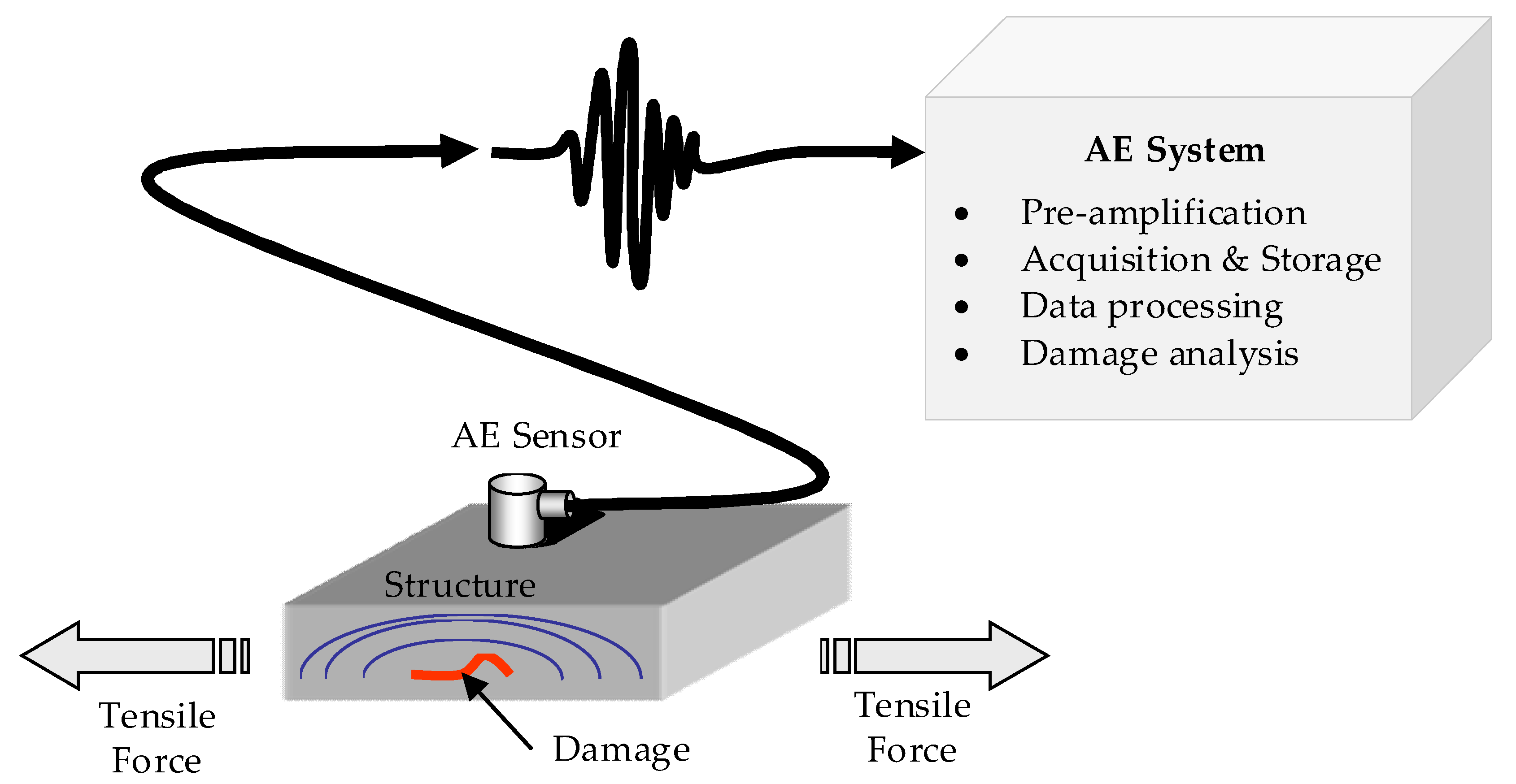
The structure diagram of AE detection theory is shown in Figure 1. When any damage occurs in the structure under the action of external forces, a transient wave which is the result of the sudden release of stored energy, propagates from the damage location and eventually reaches the surface of the structure. The surface displacement can be converted into an electrical signal by an AE sensor, and the sensor signal can be pre-amplified, acquired, processed and analyzed by the AE system.
2.1. The EWT Method
As shown in Figure 1, data processing is an important procedure in the AE system. The aim of EWT method was to extract the signal modes, therefore it could be applied to process the AE signals. The EWT process contains three important aspects: (1) in segmenting the spectrum of the signal, the first step was to detect all the local maxima of the spectrum, then get the boundaries which were the midpoint of two consecutive maxima, using the algorithm given in Equation (1); (2) constructing the empirical wavelets by defining a bank of wavelet filters composed of one low-pass filter and N − 1 band filters based on the boundaries, which is given in Equations (2)–(5); (3) extracting the empirical modes by applying the wavelet filter banks to divide the signal into frequency sub-bands. More detailed information can be found in reference [28].
where is the segmentation boundaries; is the corresponding angular frequency of the local maxima.
where is the empirical wavelets, is the empirical scaling function; ensures no overlap between two consecutive segments, is an arbitrary function, they are given as follows:
2.2. The LWM-EWT Method
The process of spectrum segmentation is the basis and is very important for the EWT algorithm to achieve ideal separation results. When the signal has a relatively obvious peak frequency, the above-mentioned segmentation method is effective. However, when AE signals from the damage characteristics that have some frequency bands are processed, some local maxima which are from noise or frequency dispersion might appear and be mistakenly kept in the peak frequency sequence, then this method may lead to a false segmentation. Another drawback of the spectrum segmentation is that the boundary method, which is to obtain the midpoint of the two adjacent local maxima, is too simple, especially when the distance of two local maxima is far, and the extracted signal bandwidth will be too wide.
When the EWT method is used to process the AE signals, a modified method is proposed in this paper. This method can avoid the improper segments, detect the local maxima and obtain the frequency boundaries. The method is the local window maxima (LWM) segmentation algorithm which means finding the local maxima in a proper window which can be determined according the damage signal features. The process is as follows:
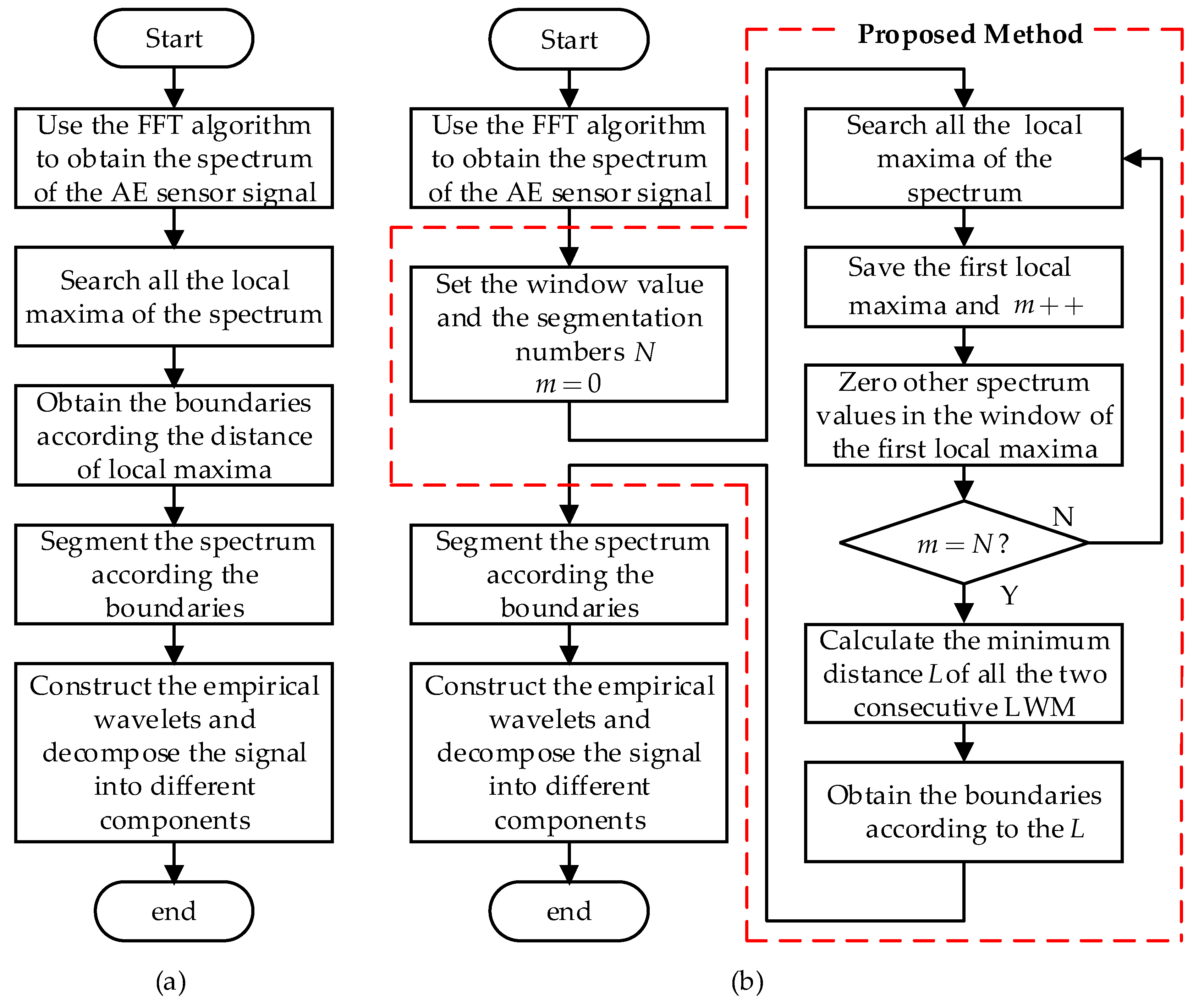
- Use the FFT algorithm to obtain the spectrum of the AE sensor signal.
- According to the characteristics of the AE signals from composite structures, set the window value W and the segmentation numbers N (the two parameters are discussed in Section 3).
- Set the counts of local window maxima m = 0.
- Search all the local maxima of the signal spectrum.
- Sort descending the local maxima, save the first one as one LWM and set .
- Center on the LWM which is generated from step 5 and zero other spectrum values in .
- If is not equal , go back to step 4.
- Calculate the minimum distance L of all the two consecutive LWM.
- Obtain the boundaries according to the L and each LWM, for example, if LWM-1 is the first LWM and is the frequency of LWM-1, then boundaries for LWM1 are given in Equation (6):
The procedure of the LWM-EWT method is compared with the EWT method in Figure 2 and the improvements are highlighted in the dotted red area.
The purpose of the proposed method is to find the proper local maxima and how to obtain boundaries. Here the details are discussed. To detect the LWM, the idea is that the most important maxima in the magnitude of the Fourier transform of the sensor signal is significantly larger than the other existing maxima.
2.2.1. Picking Out the LWM
Here the example how to pick out the first LWM is given to explain the detection theory of LWM. First, the detected local maxima in the magnitude of the Fourier spectrum is sorted descending and the set can be described as:
where is one of the local maxima.
The corresponding angular frequencies of these maxima are given as:
where is the angular frequency of .
If is the first LWM, denoted by LWM-1, then zero the amplitude that the frequency is in the window of , except for the center frequency of . The equation is as follows:
where is the spectrum amplitude; is the angular frequency.
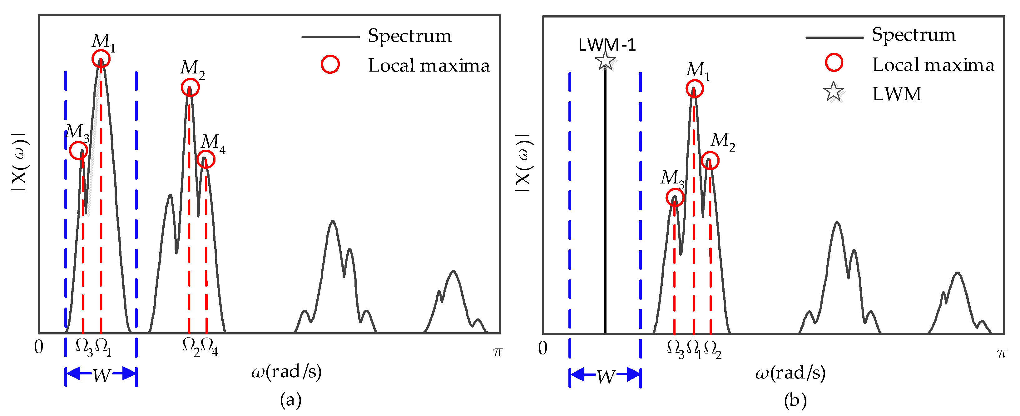
When there are four LWM that need to be detected, the detection process of the first LWM is illustrated in Figure 3.
2.2.2. Detecting the Boundaries
All the LWM can be obtained based on the solution in Section 2.2.1, then the minimum distance of all the two adjacent LWM can be calculated by the following equation:
And the boundaries are given as:
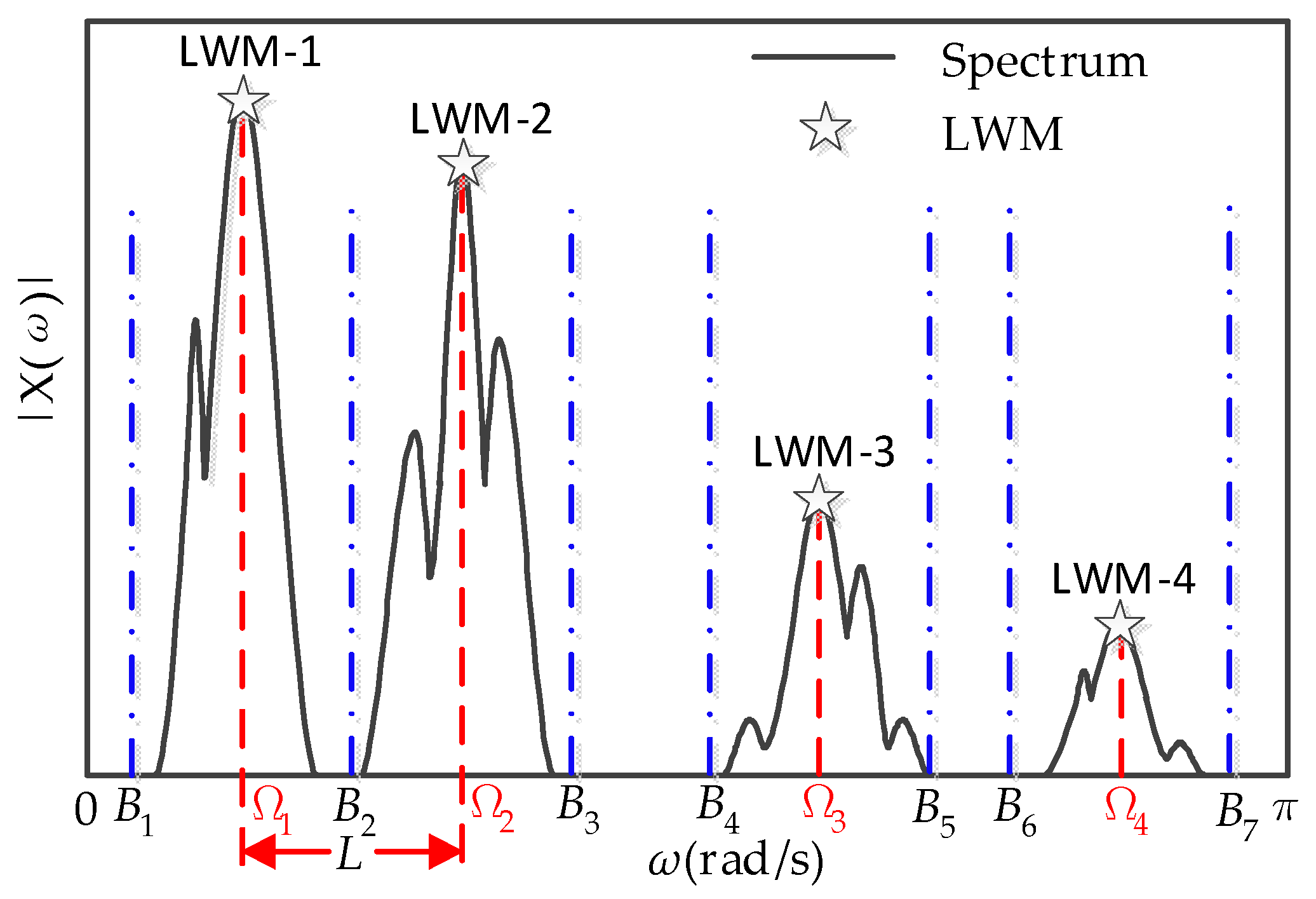
when there are four LWM, the boundaries are shown in Figure 4.
3. Numerical Simulation Signal Analysis and Discussion
A numerical simulation is done to verify the proposed method. Without loss of generality, the modulated sine burst, which is a narrow-band signal, is employed in the simulation. From [36], the simulation signal can be expressed as follows:
where A is the signal amplitude; is the central frequency; is the time; is the Heaviside step response; is the wave numbers.
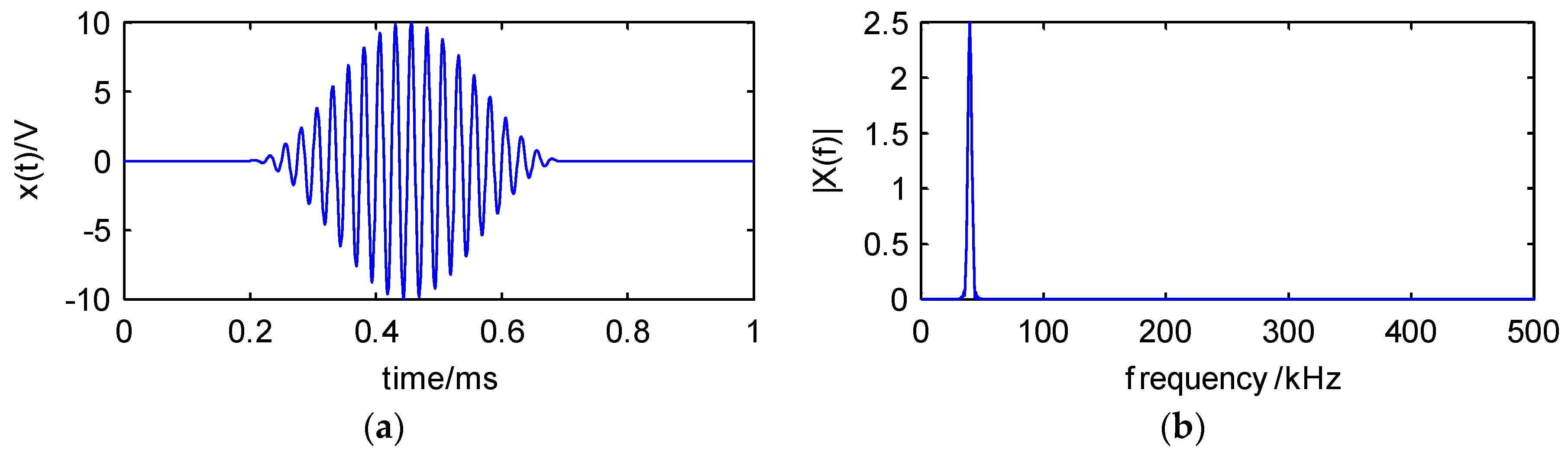
For example, when t = 1 ms, and the sample rate is 1 MHz, the simulation signal is shown in Figure 5.
During the simulation process, the first step is to generate the mixed signal according to the Equation (12), if it is composed of n different modes, then it can be expressed as:
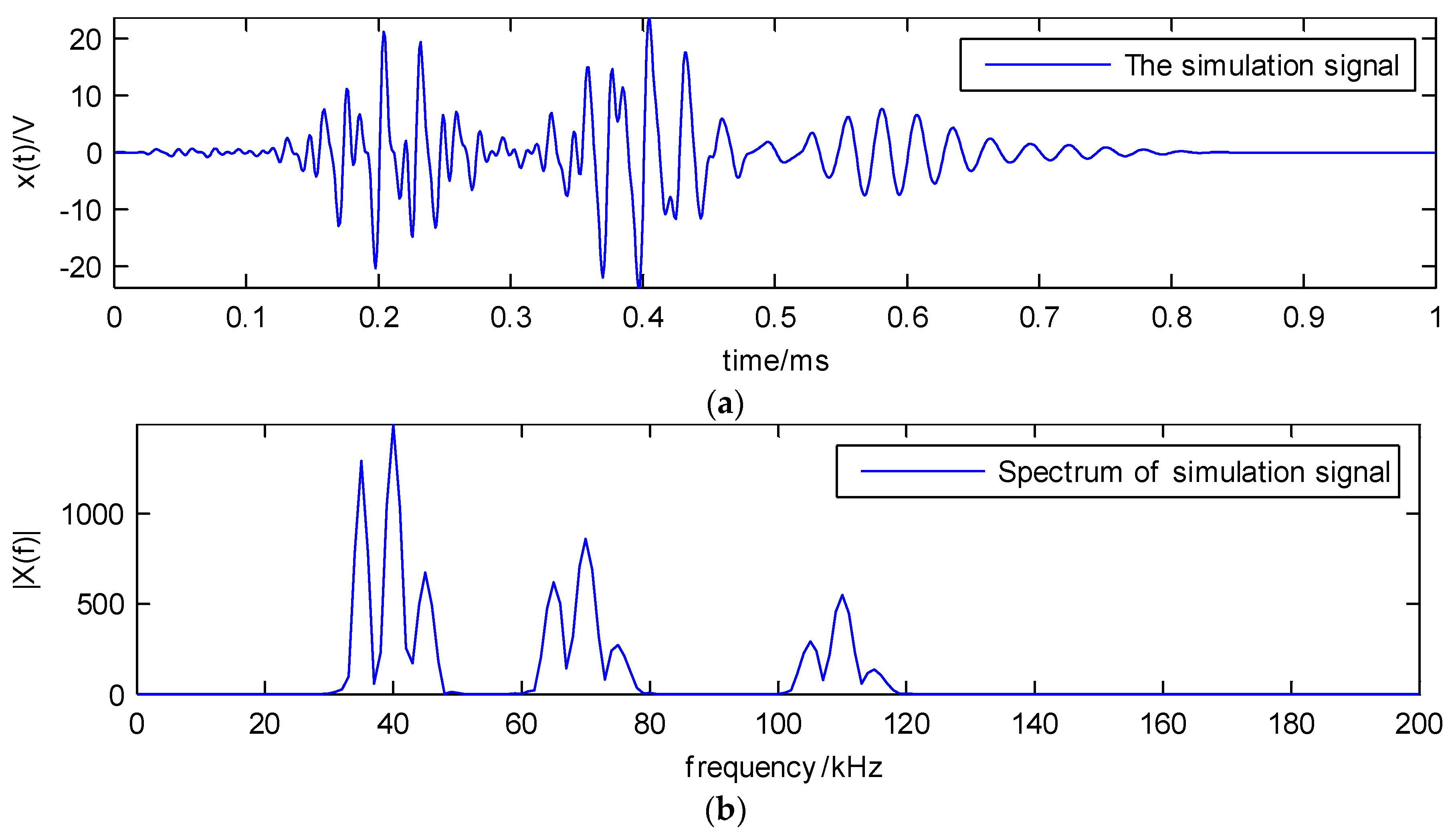
When n = 9, and all the simulation parameters are as given in Equation (14), the simulated sensor signal is shown in Figure 6.
It is difficult to separate the simulated sensor signal into different components only from the waveform information in Figure 6a. But there are nine different frequency peaks in the spectrum (Figure 6b). Here the parameters of window value and segmentation numbers will be discussed. The window value relies on the practical requirement and experience, for example if the three components of 35, 40 and 45 kHz can be regarded as only one component, the window will be 10 kHz, but the segmentation numbers can be obtained by the energy of the component, if the energy proportion of one component is larger than a specify value, then the component can be considered as a segmentation.
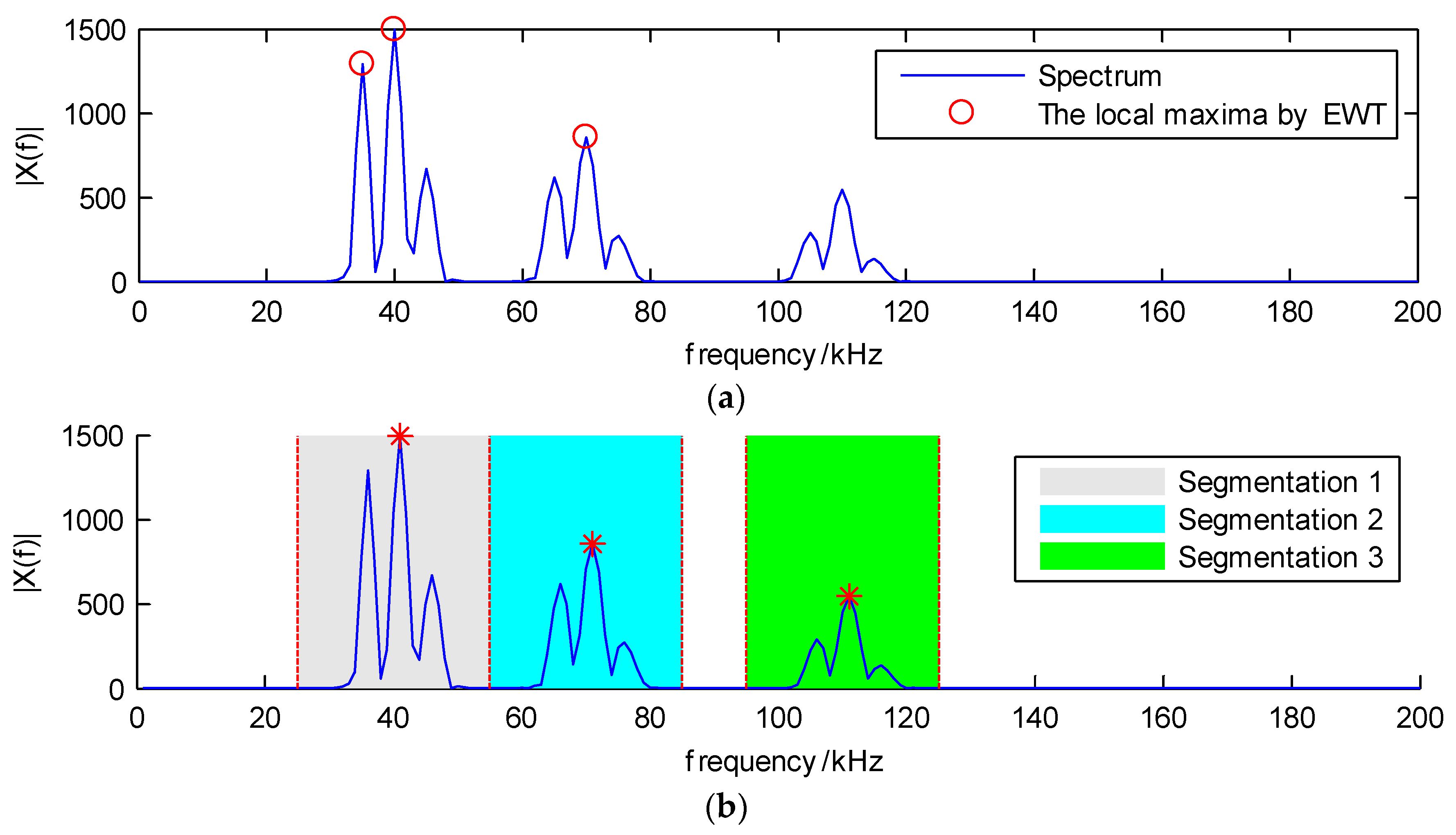
When the window value is 10 kHz and the segmentation numbers are three, the detected local maxima of the original EWT and the LWM method, which are the red circles and red stars, respectively, are illustrated in Figure 7. As shown in Figure 7a, the first two local maxima are very close, which may generate two narrow bands in the decomposition results, and this is not applicable for analyzing the non-stationary AE signals which have the dispersion phenomenon when they propagate on the composite structure. Therefore, compared with the original EWT method, the proposed LWM approach gives better results for the local maxima, which are shown in Figure 7b.
Based on the local maxima, segmentation boundaries are obtained which are the red dashed lines in Figure 7b, and three spectrum segmentations are shown, denoted by the gray, cyan and green colors. This indicates that the proposed LWM algorithm performs well in searching for the local maxima and segmenting the spectrum.
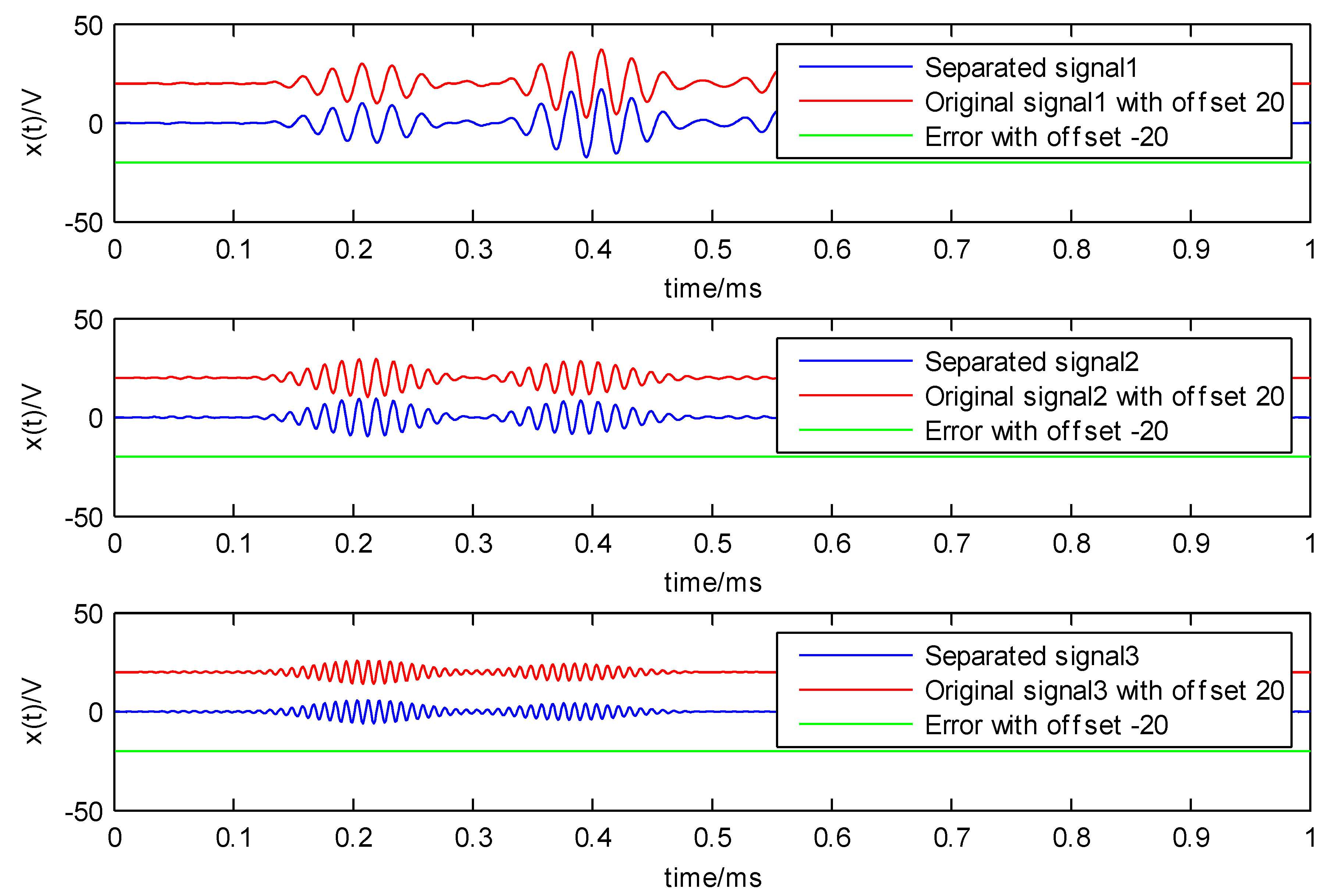
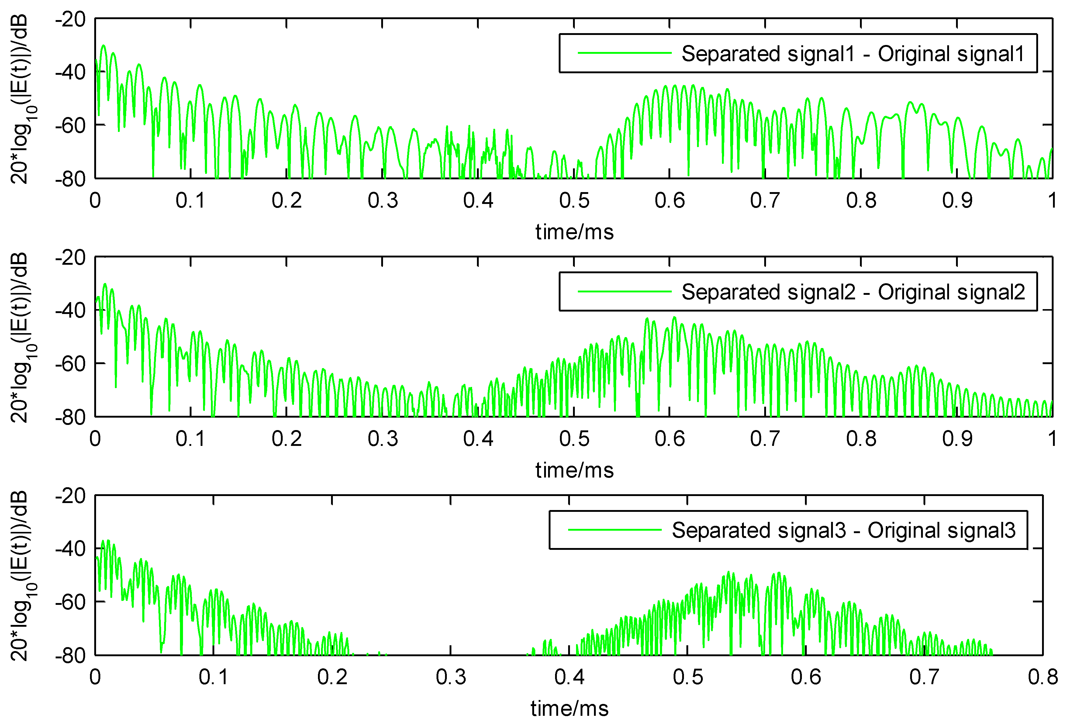
The decomposition results of the LWM-EWT method are depicted in Figure 8 and Figure 9, in order to have a more obvious contrast, the original signals with offset of 20 V (each of which is the mixed signal of three nearest frequency simulation signal), the separated signals and error with offset of −20 V between them are depicted in one figure.
4. Experimental Results and Discussion
4.1. Pencil-Lead Breaks Experiment
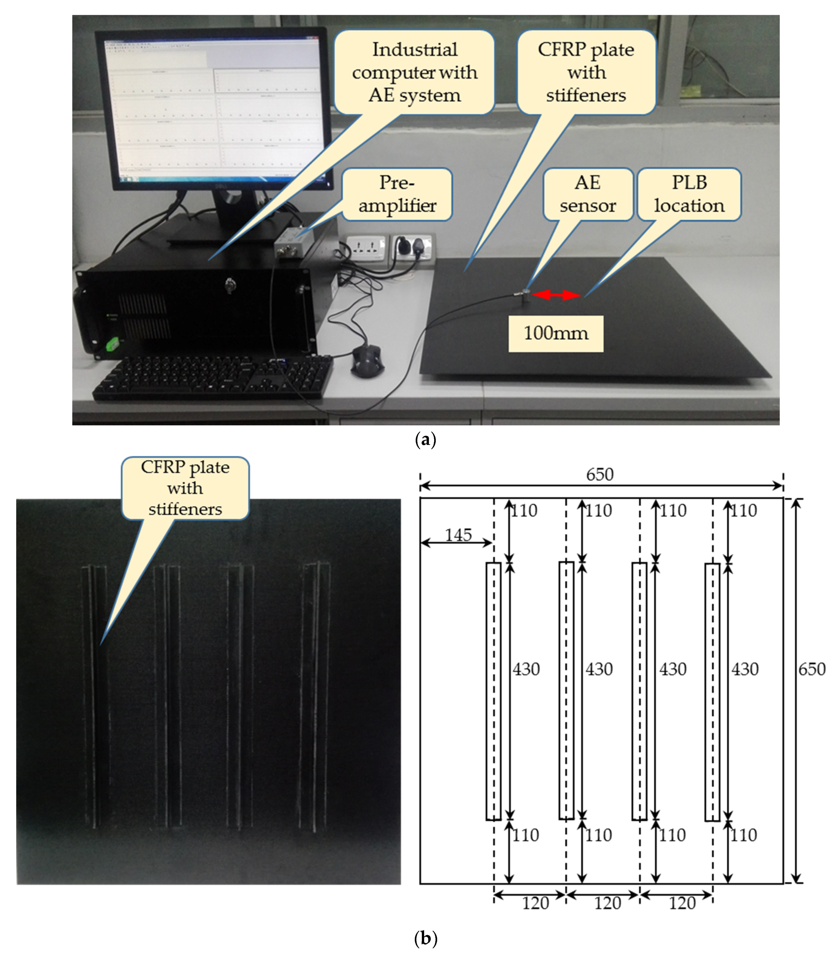
Pencil-lead breaks (PLB) in plates were used as the typical AE test source in literature [19,21]. In order to verify the effectiveness of the proposed approach, here a PLB signal is captured by an AE detection system. The schematic diagram of the experimental system is displayed in Figure 10. It consists of a CFRP plate, PLB (on the top surface of the plate), AE sensor, pre-amplifier, AE system and industrial computer. The AE sensor is mounted on the top surface of CFRP plate, and the AE signal is captured in the experiment. During the experiment, the original AE signal is amplified by 40 dB, and the sample rate is 10 MHz.
The detailed information of the experimental system is shown in Table 1.
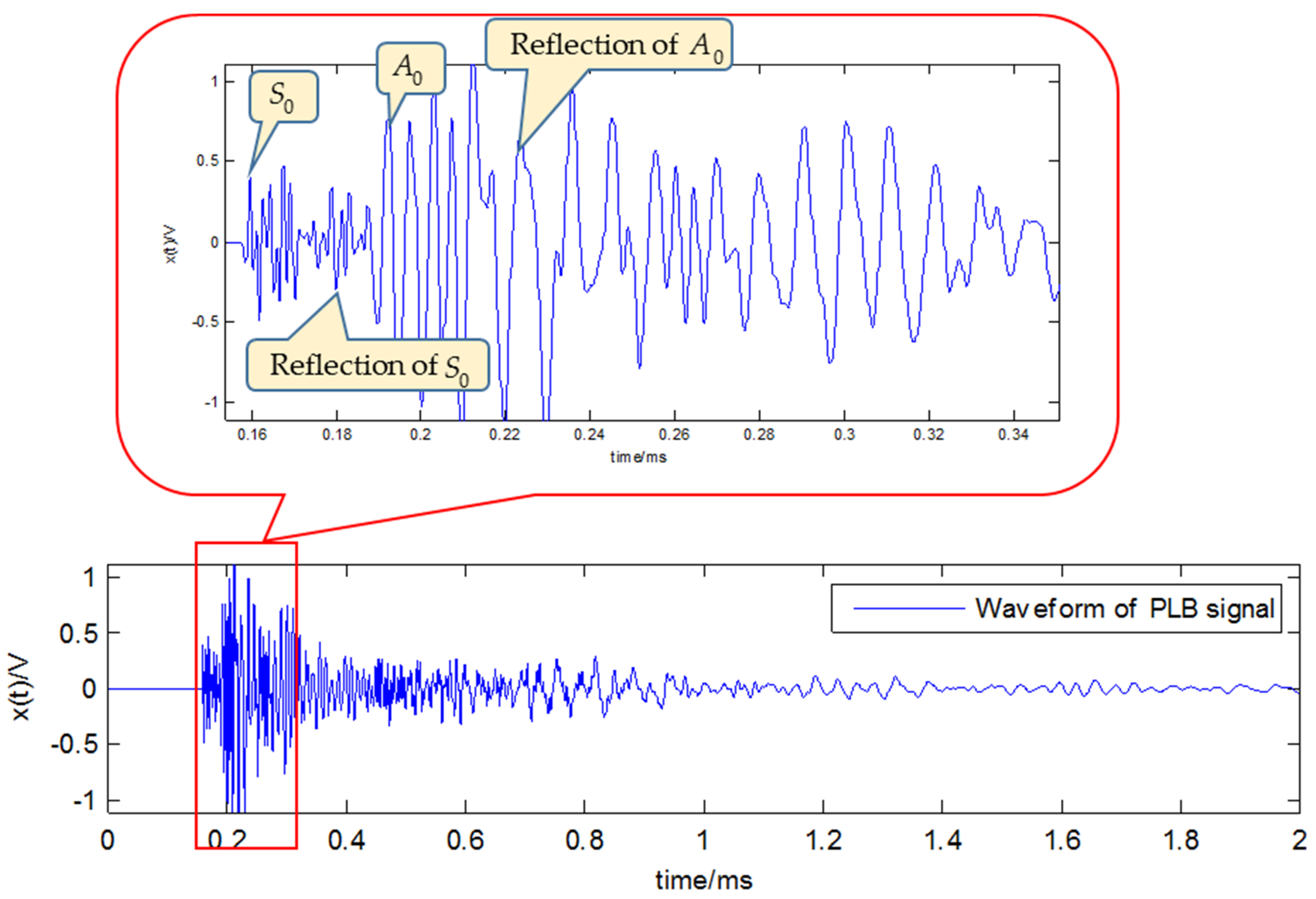
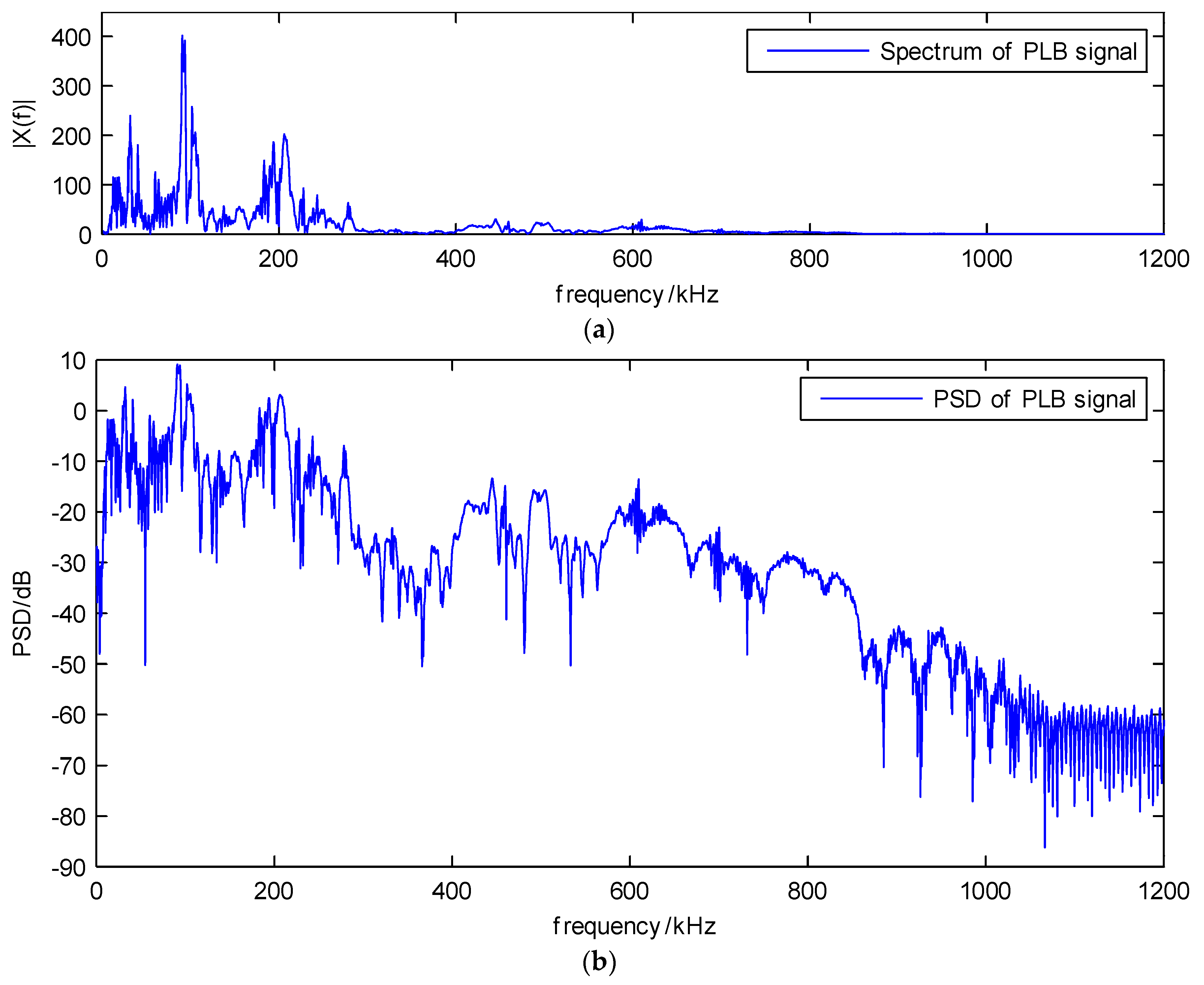
From the acquired AE signal, the waveform and spectrum of PLB can be obtained. The waveform in Figure 11 shows the duration of PLB signal is about 0.4 ms, and it can be seen that both the extensional mode and flexural mode are present. There are many peak frequencies, due to the big difference of the amplitude, the high frequency components are not obvious in Figure 12a, but from the power spectral density (PSD) in Figure 12b, it can be seen that the three main spectrum bands are in the near zone of 100, 200 and 500 kHz. Then the main difficulty of analyzing this signal would be separating the three main components from the high level of noise, especially the nearby peak frequencies.
When the window value is 50 kHz and the segmentation numbers are three, the detected local maxima using the original EWT and LWM methods are shown in Figure 13, where they are denoted by the red circles and red stars, respectively.
In Figure 13a, the three maxima are very close to each other, they should not be separated to three different components, but by using the traditional method, they could be roughly separated. Therefore, the results through the proposed LWM method are better than the original EWT, where the three local maxima are located in the three main frequency bands. The separated results based on the proposed LWM-EWT method are depicted in Figure 14. It contains the waveform and spectrum of three dominant components decomposed from the PLB signal.
4.2. Three-Point Bending Experiment
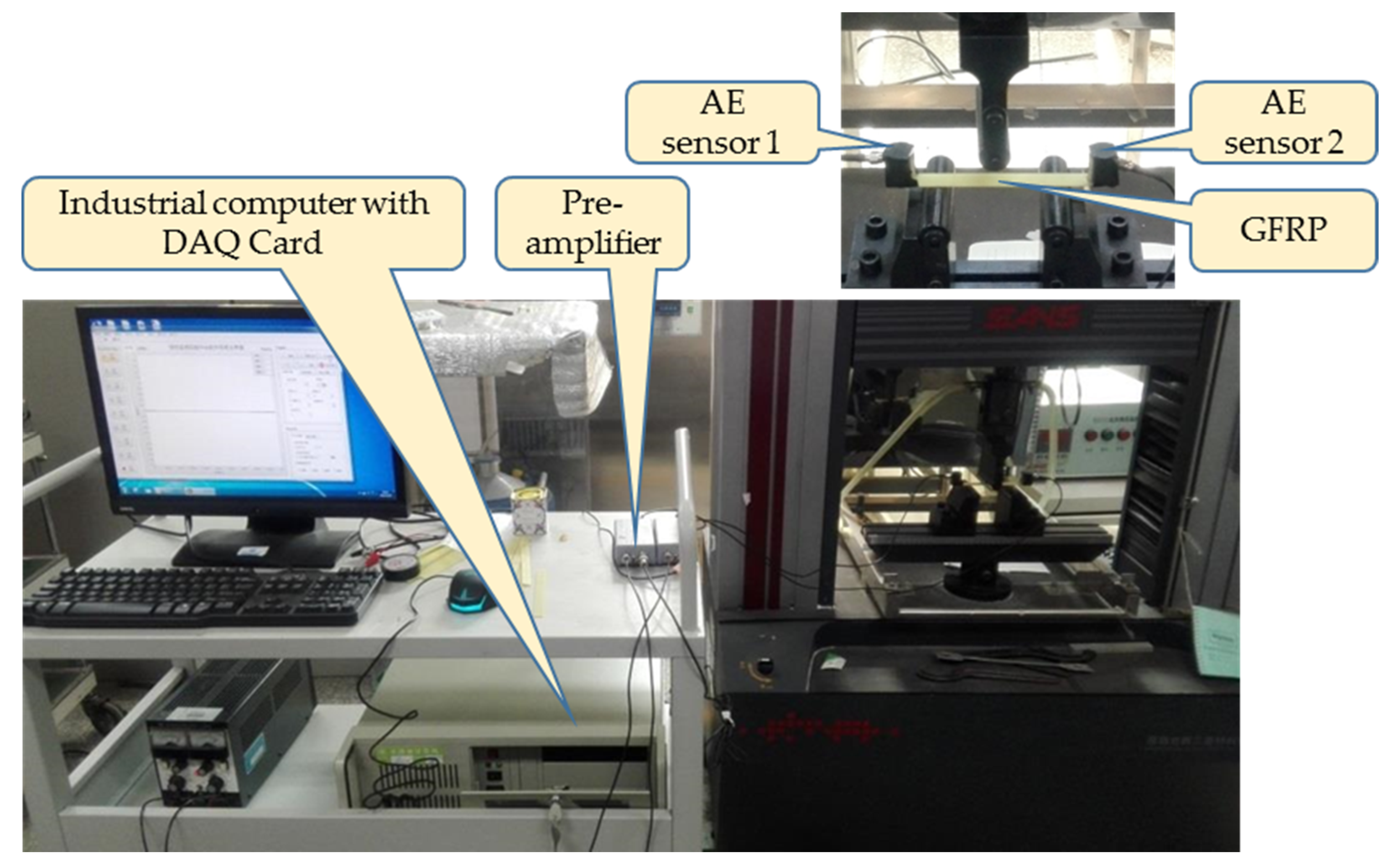
According to the ASTM-D790-10 specification, a specimen of glass fiber reinforced plastics (GFRP) laminates plate with dimension of 120 mm × 15 mm × 2.5 mm is tested on the three-point bending load rig. The experimental system is seen in Figure 15.
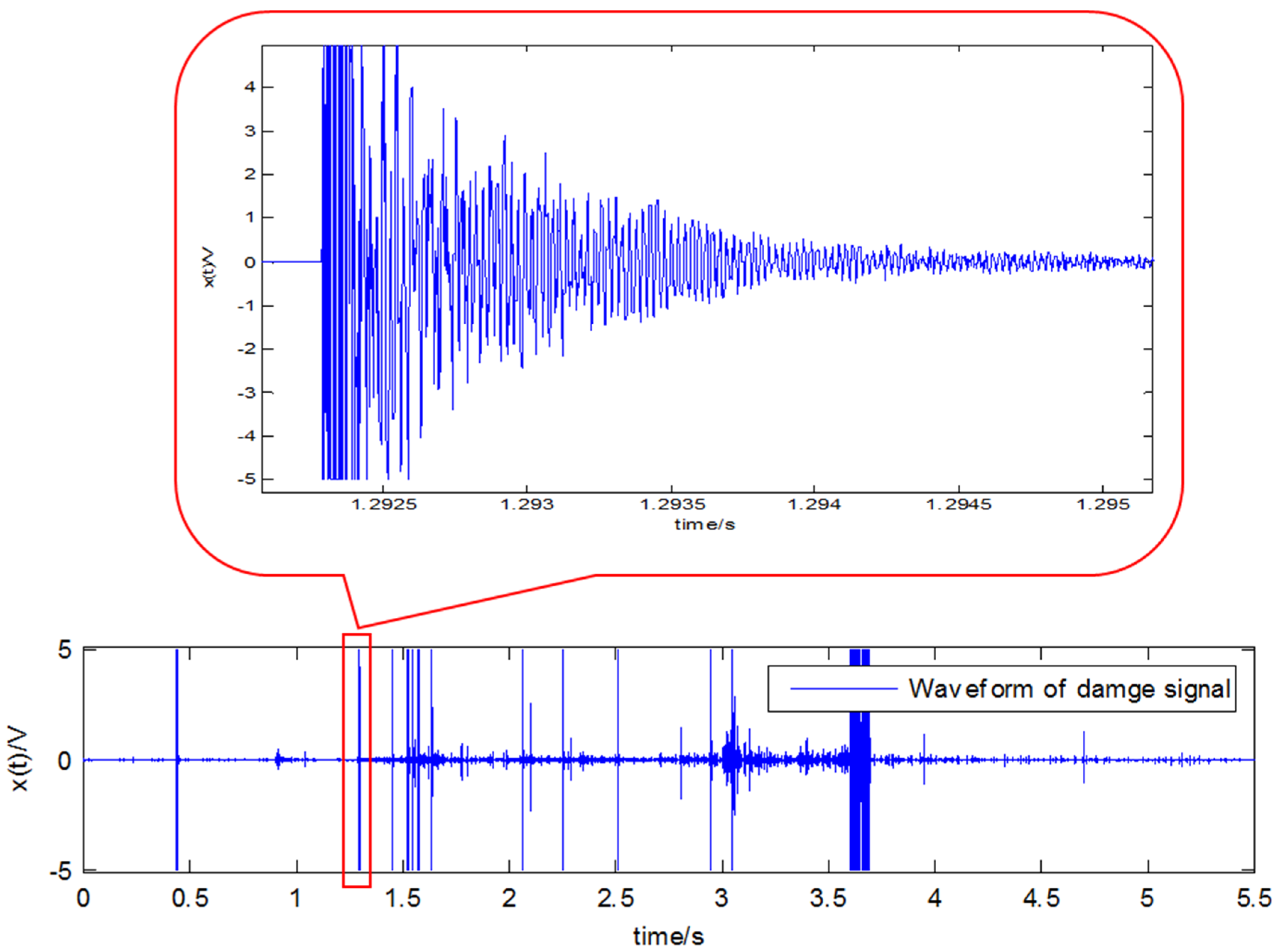
During the experimental process, which lasts about 5 s, two AE sensors are used to monitor the damage signals, and the waveform of sensor 1 is seen in Figure 16.
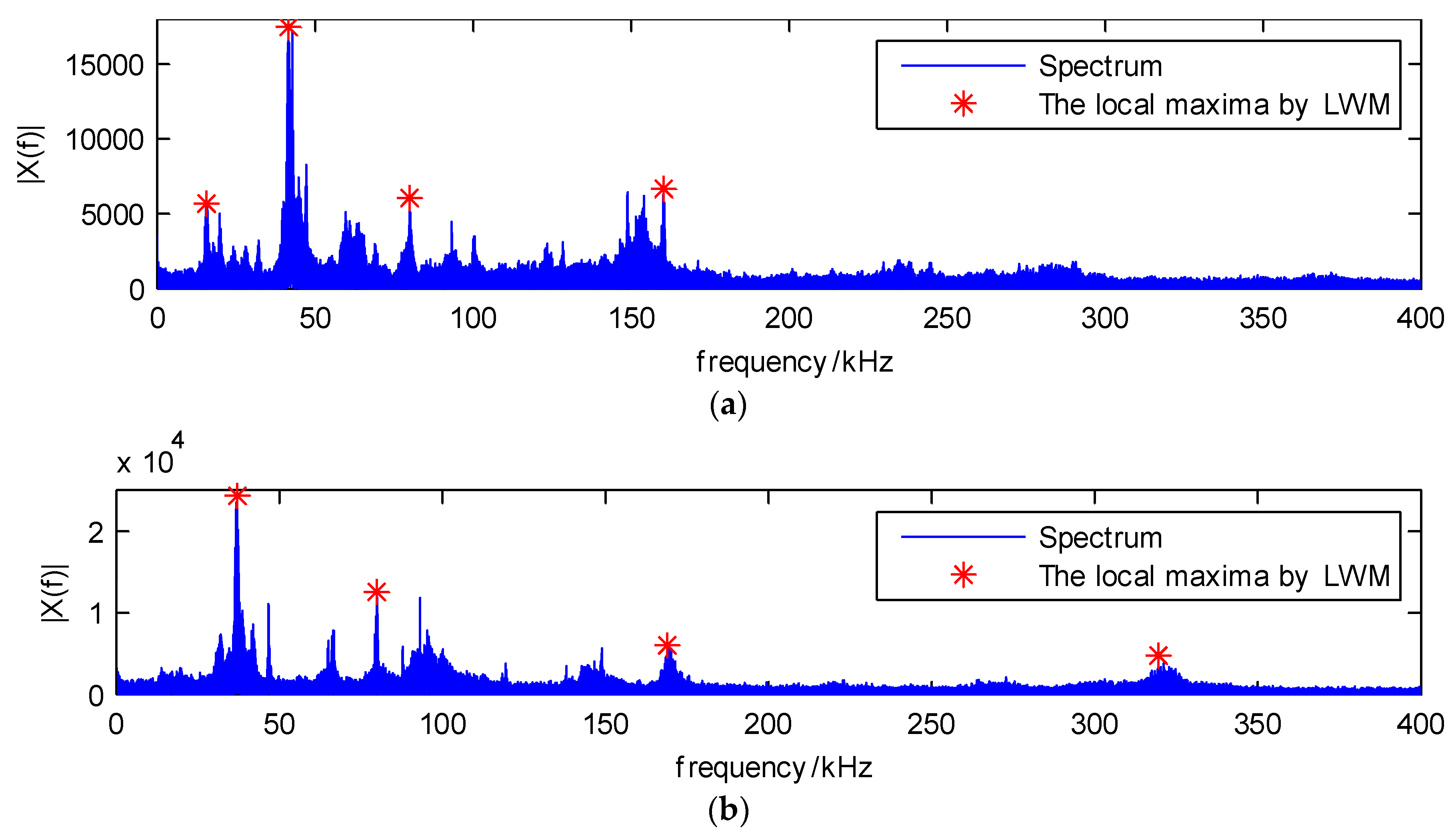
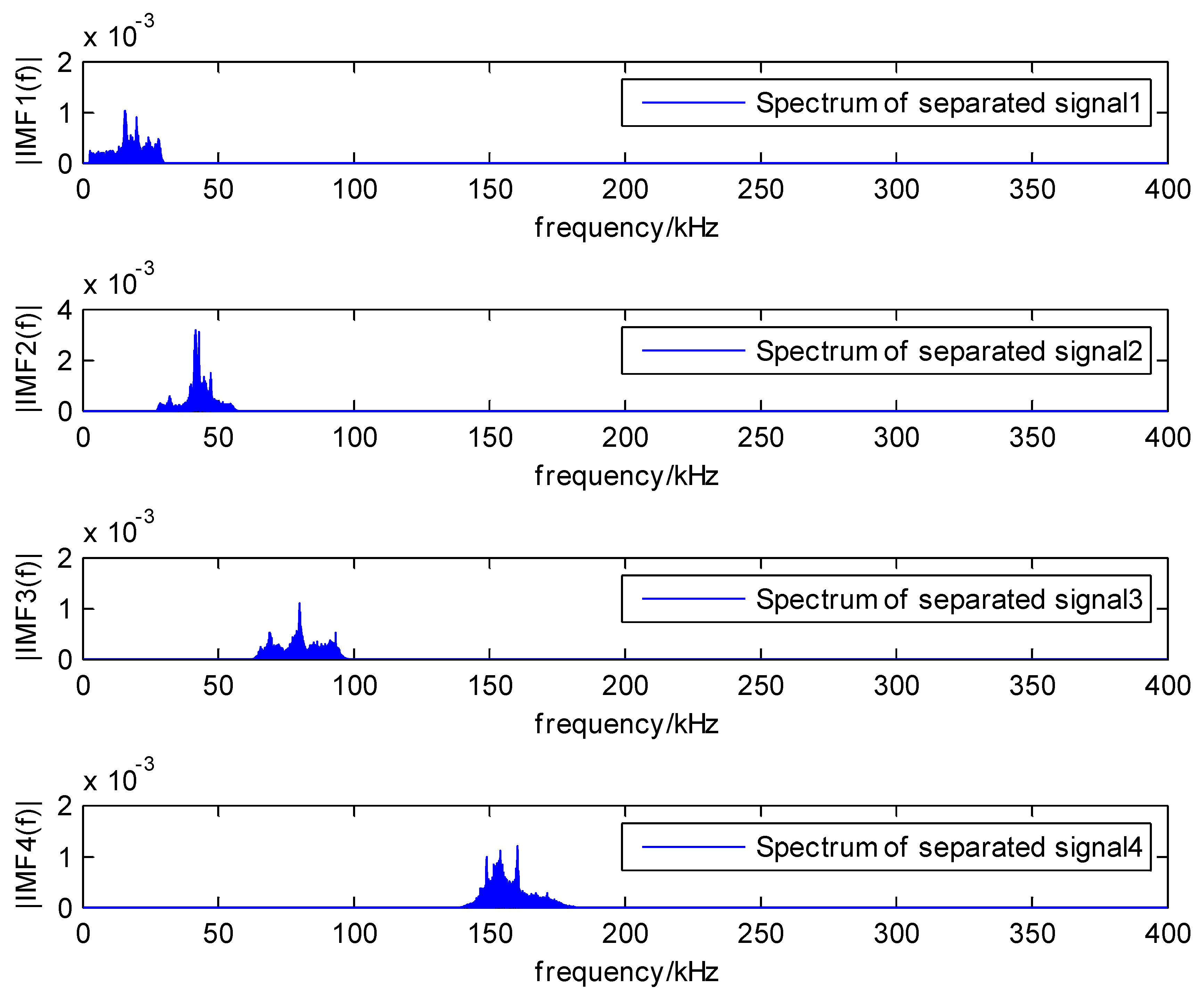
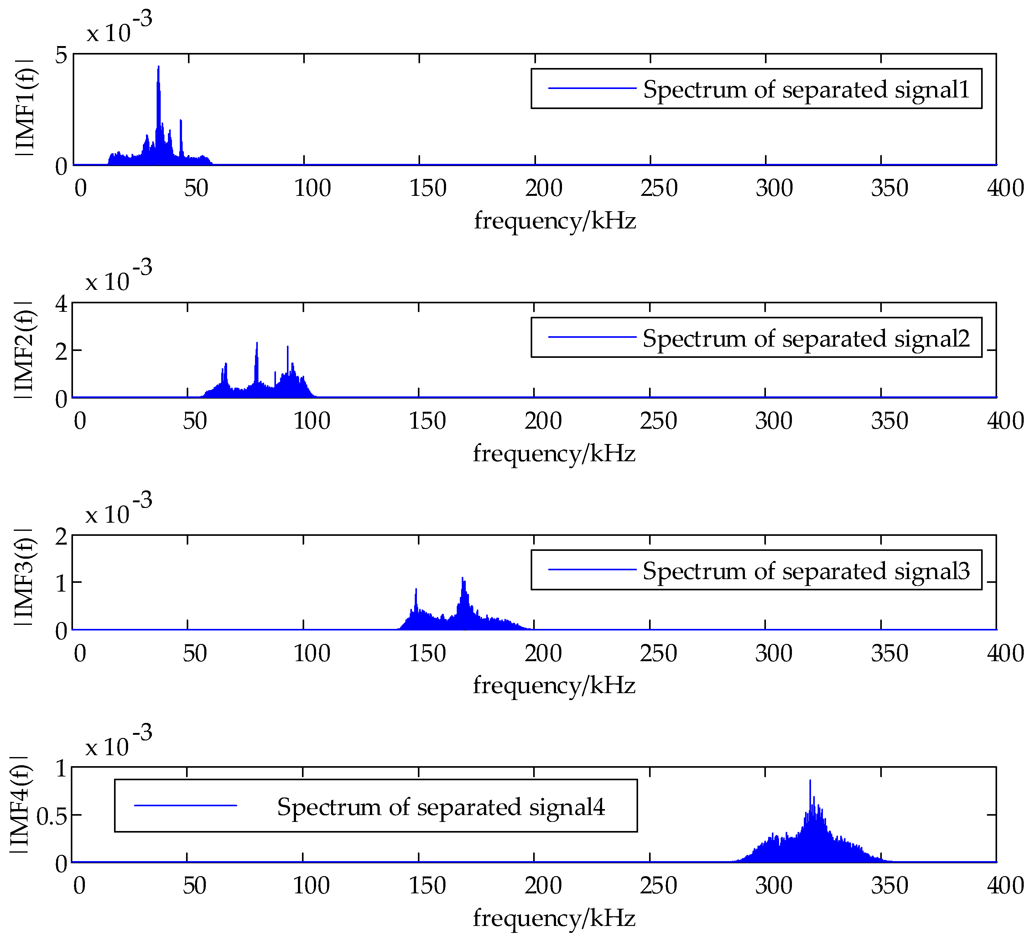
The load speed is 5 mm/min, AE signals happen on the load force of 200 N, and the plate is broken when the load force is about 220 N. The spectrum and local maxima by the proposed method are shown in Figure 17. In addition, the spectrum of separated signals from two sensors are depicted in Figure 18 and Figure 19.
5. Conclusions
This paper presents a novel signal decomposition method which is applied to AE signal processing. To eliminate the impact of noise interference or frequency dispersion, the LWM segmentation approach is used to search the dominant local maxima and the segmentation boundaries. Through the presented algorithm, useful components for damage analysis are decomposed. The decomposition results from the simulation and practical experiment show that the meaningful empirical modes, which are more reflective of damage characteristics, are obtained. Additionally, compared with the original EWT, components decomposed by the proposed LWM-EWT are much more reasonable for the AE signals. Since the frequency of AE signals can be influenced by different structures, further research work should concentrate on acquiring more signals from other structures, to validate the proposed method.
Author Contributions
Conceptualization, S.D. and M.Y.; Methodology, Q.W.; Software, S.D. and Q.W.; Validation, S.D., M.Y. and Z.L.; Formal Analysis, S.D.; Investigation, S.D.; Resources, S.D.; Data Curation, S.D.; Writing-Original Draft Preparation, S.D.; Writing-Review & Editing, S.D., Q.W. and Z.L.; Visualization, S.D.; Supervision, M.Y.; Project Administration, M.Y.; Funding Acquisition, M.Y.
Funding
The authors acknowledged the financial support of the National Natural Science Foundation of China (NSFC) under the Grant No. 51375030, and the special funds for improving basic condition for central universities of China
Conflicts of Interest
The authors declare no conflict of interest.
References
- Baker, A.A.B.; Kelly, D.W. Composite Materials for Aircraft Structures; American Institute of Aeronautics and Astronautics: Reston, VA, USA, 2004; p. 1. [Google Scholar]
- Zhong, Y.; Yuan, S.; Qiu, L. Multiple damage detection on aircraft composite structures using near-field MUSIC algorithm. Sens. Actuators A Phys. 2014, 214, 234–244. [Google Scholar] [CrossRef]
- Velazquez, E.; Kosmatka, J.B. Acoustic Emission Structural Health Monitoring of Laminated Composite Aircraft Structures; American Institute of Aeronautics and Astronautics Inc.: Honolulu, HI, USA, 2012; pp. 1–20. [Google Scholar]
- Farrar, C.R.; Worden, K. An introduction to structural health monitoring. Philos. Trans. R. Soc. A 2007, 365, 303–315. [Google Scholar] [CrossRef] [PubMed]
- Diamanti, K.; Soutis, C. Structural health monitoring techniques for aircraft composite structures. Prog. Aerosp. Sci. 2010, 46, 342–352. [Google Scholar] [CrossRef]
- Johnson, M.; Gudmundson, P. Broad-band transient recording and characterization of acoustic emission events in composite laminates. Compos. Sci. Technol. 2000, 60, 2803–2818. [Google Scholar] [CrossRef]
- Hamstad, M.A. A review: Acoustic emission, a tool for composite-materials studies. Exp. Mech. 1986, 26, 7–13. [Google Scholar] [CrossRef]
- Romhany, G.; Czigany, T.; Karger-Kocsis, J. Failure Assessment and Evaluation of Damage Development and Crack Growth in Polymer Composites via Localization of Acoustic Emission Events: A Review. Polym. Rev. 2017, 57, 397–439. [Google Scholar] [CrossRef]
- Yousefi, J.; Ahmadi, M.; Shahri, M.N.; Oskouei, A.R.; Moghadas, F.J. Damage Categorization of Glass/Epoxy Composite Material under Mode II Delamination Using Acoustic Emission Data: A Clustering Approach to Elucidate Wavelet Transformation Analysis. Arab. J. Sci. Eng. 2014, 39, 1325–1335. [Google Scholar] [CrossRef]
- Dahmene, F.; Yaacoubi, S.; El Mountassir, M.; Bendaoud, N.; Langlois, C.; Bardoux, O. On the modal acoustic emission testing of composite structure. Compos. Struct. 2016, 140, 446–452. [Google Scholar] [CrossRef]
- Surgeon, M.; Wevers, M. Modal analysis of acoustic emission signals from CFRP laminates. NDT E Int. 1999, 32, 311–322. [Google Scholar] [CrossRef]
- Kim, S.T.; Lee, Y.T. Characteristics of damage and fracture process of carbon fiber reinforced plastic under loading-unloading test by using AE method. Mater. Sci. Eng. A-Struct. 1997, 234, 322–326. [Google Scholar] [CrossRef]
- Benammar, A.; Drai, R.; Guessoum, A. Detection of delamination defects in CFRP materials using ultrasonic signal processing. Ultrasonics 2008, 48, 731–738. [Google Scholar] [CrossRef] [PubMed]
- Bourchak, M.; Farrow, I.R.; Bond, I.P.; Rowland, C.W.; Menan, F. Acoustic emission energy as a fatigue damage parameter for CFRP composites. Int. J. Fatigue 2007, 29, 457–470. [Google Scholar] [CrossRef]
- Prosser, W.H.; Hamstad, M.A.; Gary, J.; O’Gallagher, A. Finite Element and Plate Theory Modeling of Acoustic Emission Waveforms. J. Nondestr. Eval. 1999, 18, 83–90. [Google Scholar] [CrossRef]
- Sause, M.G.R.; Horn, S. Simulation of Acoustic Emission in Planar Carbon Fiber Reinforced Plastic Specimens. J. Nondestr. Eval. 2010, 29, 123–142. [Google Scholar] [CrossRef]
- Sause, M.G.R.; Hamstad, M.A.; Horn, S. Finite element modeling of conical acoustic emission sensors and corresponding experiments. Sens. Actuators A Phys. 2012, 184, 64–71. [Google Scholar] [CrossRef]
- Sause, M.G.R.; Hamstad, M.A.; Horn, S. Finite element modeling of lamb wave propagation in anisotropic hybrid materials. Compos. Part B Eng. 2013, 53, 249–257. [Google Scholar] [CrossRef]
- Zelenyak, A.; Hamstad, M.A.; Sause, M.G.R. Modeling of Acoustic Emission Signal Propagation in Waveguides. Sensors 2015, 15, 11805–11822. [Google Scholar] [CrossRef] [PubMed]
- Sause, M.G.R.; Hamstad, M.A. Numerical modeling of existing acoustic emission sensor absolute calibration approaches. Sens. Actuators A Phys. 2018, 269, 294–307. [Google Scholar] [CrossRef]
- Martínez-Jequier, J.; Gallego, A.; Suárez, E.; Juanes, F.J.; Valea, Á. Real-time damage mechanisms assessment in CFRP samples via acoustic emission Lamb wave modal analysis. Compos. Part B Eng. 2015, 68, 317–326. [Google Scholar] [CrossRef]
- Yaacoubi, S.; Dahmene, F.; Bouzenad, A.; El Mountassir, M.; Aouini, M. Modal acoustic emission for composite structures health monitoring: Issues to save computing time and algorithmic implementation. Compos. Struct. 2018, 183, 338–346. [Google Scholar] [CrossRef]
- Gutkin, R.; Green, C.J.; Vangrattanachai, S.; Pinho, S.T.; Robinson, P.; Curtis, P.T. On acoustic emission for failure investigation in CFRP: Pattern recognition and peak frequency analyses. Mech. Syst. Signal Prcess. 2011, 25, 1393–1407. [Google Scholar] [CrossRef]
- McCrory, J.P.; Al-Jumaili, S.K.; Crivelli, D.; Pearson, M.R.; Eaton, M.J.; Featherston, C.A.; Guagliano, M.; Holford, K.M.; Pullin, R. Damage classification in carbon fibre composites using acoustic emission: A comparison of three techniques. Compos. Part B Eng. 2015, 68, 424–430. [Google Scholar] [CrossRef]
- Kumar, C.S.; Arumugam, V.; Sengottuvelusamy, R.; Srinivasan, S.; Dhakal, H.N. Failure strength prediction of glass/epoxy composite laminates from acoustic emission parameters using artificial neural network. Appl. Acoust. 2017, 115, 32–41. [Google Scholar] [CrossRef]
- Beheshtizadeh, N.; Mostafapour, A. Processing of acoustic signals via wavelet & Choi—Williams analysis in three-point bending load of carbon/epoxy and glass/epoxy composites. Ultrasonics 2017, 79, 1–8. [Google Scholar] [PubMed]
- Norden, E.; Huang, A.S.A.R. The Empirical Mode Decomposition and the Hilbert Spectrum for Nonlinear and Non-Stationary Time Series Analysis. Proc. Math. Phys. Eng. Sci. 1998, 1971, 903–996. [Google Scholar]
- Gilles, J. Empirical wavelet transform. IEEE Trans. Signal Process. 2013, 61, 3999–4010. [Google Scholar] [CrossRef]
- Gilles, J.; Heal, K. A parameterless scale-space approach to find meaningful modes in histograms—Application to image and spectrum segmentation. Int. J. Wavelets Multiresolut. 2014, 12, 1450044. [Google Scholar] [CrossRef]
- Amezquita-Sanchez, J.P.; Park, H.S.; Adeli, H. A novel methodology for modal parameters identification of large smart structures using MUSIC, empirical wavelet transform, and Hilbert transform. Eng. Struct. 2017, 147, 148–159. [Google Scholar] [CrossRef]
- Yuan, M.; Sadhu, A.; Liu, K. Condition assessment of structure with tuned mass damper using empirical wavelet transform. J. Vib. Control 2017, 1–18. [Google Scholar] [CrossRef]
- Kedadouche, M.; Thomas, M.; Tahan, A. A comparative study between Empirical Wavelet Transforms and Empirical Mode Decomposition Methods: Application to bearing defect diagnosis. Mech. Syst. Signal Process. 2016, 81, 88–107. [Google Scholar] [CrossRef]
- Zheng, J.; Pan, H.; Yang, S.; Cheng, J. Adaptive parameterless empirical wavelet transform based time-frequency analysis method and its application to rotor rubbing fault diagnosis. Signal Process. 2017, 130, 305–314. [Google Scholar] [CrossRef]
- Wang, D.; Zhao, Y.; Yi, C.; Tsui, K.; Lin, J. Sparsity guided empirical wavelet transform for fault diagnosis of rolling element bearings. Mech. Syst. Signal Process. 2018, 101, 292–308. [Google Scholar] [CrossRef]
- Song, Y.; Zeng, S.; Ma, J.; Guo, J. A fault diagnosis method for roller bearing based on empirical wavelet transform decomposition with adaptive empirical mode segmentation. Measurement 2018, 117, 266–276. [Google Scholar] [CrossRef]
- Shan, S.; Qiu, J.; Zhang, C.; Ji, H.; Cheng, L. Multi-damage localization on large complex structures through an extended delay-and-sum based method. Struct. Health Monit. 2016, 15, 50–64. [Google Scholar] [CrossRef]
Figure 1.
The structure diagram of AE detection theory.

Figure 2.
Flowcharts of (a) the EWT method and (b) the proposed LWM-EWT method.

Figure 3.
The detection process of the first LWM. (a) Detect the four local maxima and determine the window. (Red circles are the local maxima; blue dashed lines are the boundaries of the window.); (b) zero the amplitude in the window, obtain the first LWM which is denoted by pentagram, and redetect the other three local maxima which are denoted by the red circles.

Figure 4.
The detected boundaries which are denoted by the blue dot-dashed lines, the four LWM and the minimum distance of two adjacent LWM.
Figure 4.
The detected boundaries which are denoted by the blue dot-dashed lines, the four LWM and the minimum distance of two adjacent LWM.

Figure 5.
The (a) waveform and (b) spectrum of the simulation signal.

Figure 6.
The (a) waveform and (b) spectrum of simulation signal which is generated by adding 9 different modulated sine burst signals together (the simulation parameters are in Equation (14) and the expression of each signal is in Equation (12)).
Figure 6.
The (a) waveform and (b) spectrum of simulation signal which is generated by adding 9 different modulated sine burst signals together (the simulation parameters are in Equation (14) and the expression of each signal is in Equation (12)).

Figure 7.
Local maxima by (a) the original EWT method denoted by red circles and (b) the LWM method denoted by red stars; the spectrum segmentation results are shown by the color of gray, cyan and green.
Figure 7.
Local maxima by (a) the original EWT method denoted by red circles and (b) the LWM method denoted by red stars; the spectrum segmentation results are shown by the color of gray, cyan and green.

Figure 8.
Decomposition signals of the proposed LWM-EWT method: the red curves are the original signals (with offset of 20 V); the blue curves are the separated signals and the green curves are the error (with offset of −20 V) between separated signals and original signals.
Figure 8.
Decomposition signals of the proposed LWM-EWT method: the red curves are the original signals (with offset of 20 V); the blue curves are the separated signals and the green curves are the error (with offset of −20 V) between separated signals and original signals.

Figure 9.
The difference value between separated signals and original signals calculated by 20*log_10(|E(t)|), the difference values are all less than 0.1 V.
Figure 9.
The difference value between separated signals and original signals calculated by 20*log_10(|E(t)|), the difference values are all less than 0.1 V.

Figure 10.
(a) The experimental system of PLB and (b) the configuration of CFRP plate with T stiffeners.
Figure 10.
(a) The experimental system of PLB and (b) the configuration of CFRP plate with T stiffeners.

Figure 11.
The waveform of the PLB signal.

Figure 12.
(a) The spectrum and (b) the PSD of PLB signal. (Include three different main spectrum bands, which are near the 100, 200 and 500 kHz marks).
Figure 12.
(a) The spectrum and (b) the PSD of PLB signal. (Include three different main spectrum bands, which are near the 100, 200 and 500 kHz marks).

Figure 13.
Local maxima of (a) the original EWT method and (b) the proposed LWM method.

Figure 14.
(a) The waveforms and (b) the spectrum of separated signals by the LWM-EWT method.

Figure 15.
The three-point bending load experimental system.

Figure 16.
The damage signal waveform of sensor 1.

Figure 17.
The spectrum and local maxima of (a) sensor 1 and (b) sensor 2.

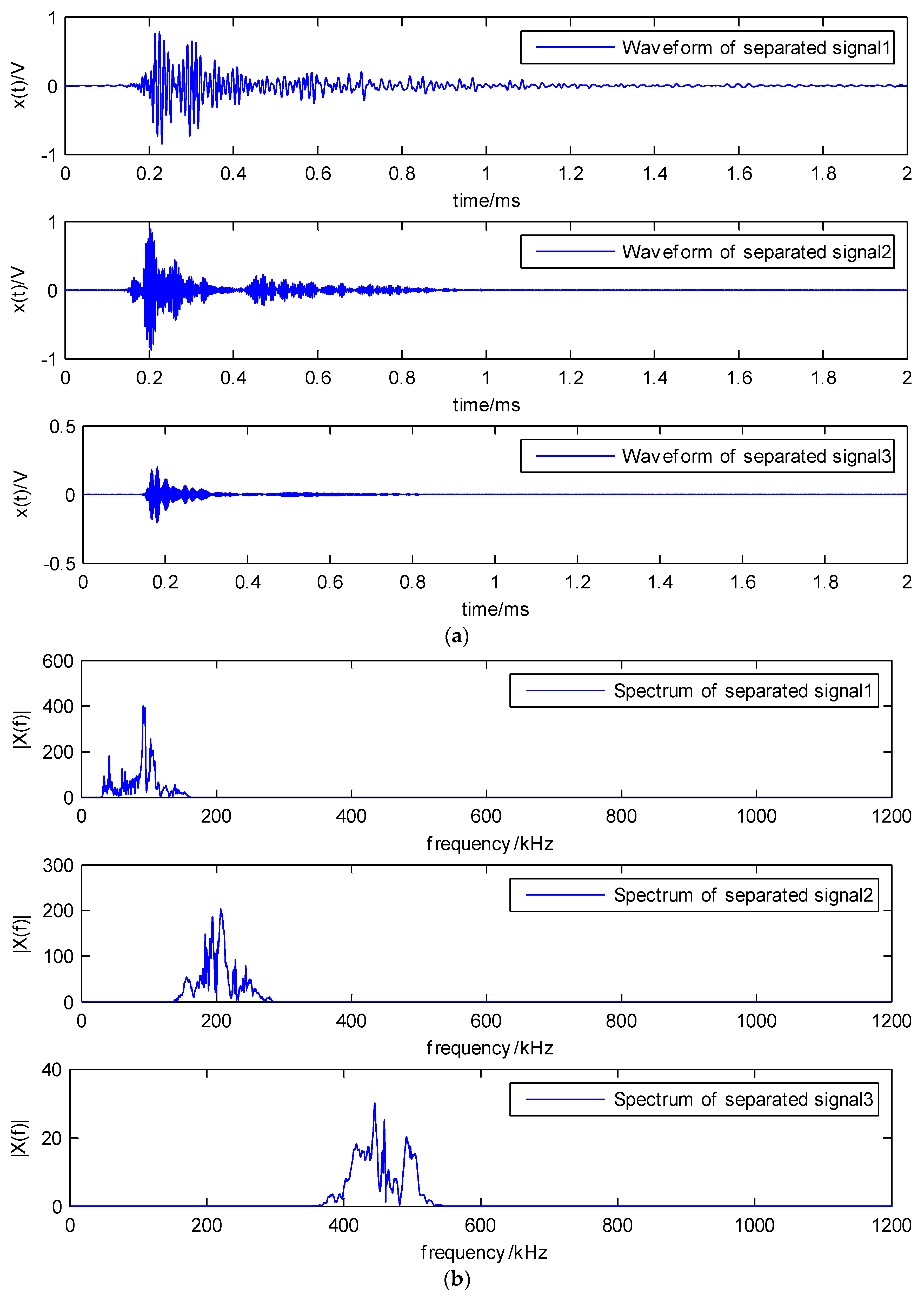
Figure 18.
The spectrum of separated signals of sensor 1.

Figure 19.
The spectrum of separated signals of sensor 2.


Table 1.
The detailed information of the experimental system.
| Name | Type | Parameter |
|---|---|---|
| CFRP plate with stiffeners | TR50S12L | 650 mm × 650 mm × 3 mm, 20 layers, [0, 90]10S; T shape stiffeners (cross section): 40 mm × 20 mm × 3 mm |
| Pencil-lead | Mitsu Nano Dia | Diameter: 0.5 mm |
| AE sensor | PAC 1 WS α | Wide-band (WD) Sensor; Operating Frequency Range: 100–1000 kHz; Temperature Range: −65–175 °C. |
| Pre-amplifier | PAC 2/4/6 | Gain Selectable: 20/40/60 dB Bandwidth: 10 kHz–2.5 MHz (20 dB), 10 kHz–2.0 MHz (40 dB), 10 kHz–900 kHz (60 dB); Temperature Range: −40–65 °C |
| AE system | PAC PCI-2 | 2 simultaneous channels, 18 bit resolution, 40 MS/s |
| Industrial computer | IEI RACK-360GBATX | E5800 3.2 GHz, 4G memory, 7 PCI slots |
1 Physical Acoustics Corporation.
© 2018 by the authors. Licensee MDPI, Basel, Switzerland. This article is an open access article distributed under the terms and conditions of the Creative Commons Attribution (CC BY) license (http://creativecommons.org/licenses/by/4.0/).
Share and Cite
MDPI and ACS Style
Dong, S.; Yuan, M.; Wang, Q.; Liang, Z. A Modified Empirical Wavelet Transform for Acoustic Emission Signal Decomposition in Structural Health Monitoring. Sensors 2018, 18, 1645. https://0-doi-org.brum.beds.ac.uk/10.3390/s18051645
AMA Style
Dong S, Yuan M, Wang Q, Liang Z. A Modified Empirical Wavelet Transform for Acoustic Emission Signal Decomposition in Structural Health Monitoring. Sensors. 2018; 18(5):1645. https://0-doi-org.brum.beds.ac.uk/10.3390/s18051645
Chicago/Turabian StyleDong, Shaopeng, Mei Yuan, Qiusheng Wang, and Zhiling Liang. 2018. "A Modified Empirical Wavelet Transform for Acoustic Emission Signal Decomposition in Structural Health Monitoring" Sensors 18, no. 5: 1645. https://0-doi-org.brum.beds.ac.uk/10.3390/s18051645
Note that from the first issue of 2016, this journal uses article numbers instead of page numbers. See further details here.