This section presents the results of the implementations of the KNN-based filtering algorithm by evaluating different sets of parameters, analyzing both the computational times and the classification accuracy.
4.1. KNN Window Search Optimization Results with Euclidean Distance
Section 3.1 described an important optimization introduced in the serial and parallel implementations concerning the computation of the distances between pixels inside a window and not within the entire image. Reducing the space where the algorithm evaluates the distances ensures a significant decrease of the computational time, as shown in
Table 2. In particular, the table provides the execution times for all the images, considering both the case in which the neighbors are searched within the entire image (
EI) and within a window of 14 rows (
WSize14). The speedup obtained with the optimization has been also included. In addition, this table shows the total number of pixels of each image and the number of pixels inside the smallest and the biggest window in the
WSize14 implementation. The times refer to tests where the Euclidean distance has been considered. The simulations of the serial code have been carried out on an Intel i7 processor, working at 3.50 GHz, equipped with 16 GB RAM. The execution times shown in the following tables have been measured using the clock routine included in the
time.h header file.
Data presented in
Table 2 show that this optimization allows a huge decrease in the execution times. For example, considering the biggest image of the dataset, P1C2, the time of the implementation for the entire image is 19,135.58 s (about 5 h and 30 min). On the contrary, considering a window of 14 rows, this time decreases to 509.16 s (about 8 min). The reason of this huge time difference is that, when the algorithm has to consider the entire image, it needs to compute a number of distances equal to (264,408–1) for each pixel, where 264,408 is the number of pixels of the P1C2 image. However, with the window technique, the algorithm computes a number of distances that, for the same image, varies from (3864–1) to (7728–1), where 3864 and 7728 are the number of pixels inside the windows with the minimum and the maximum sizes, respectively (depending whether the pixel is in the borders or in the center of the image). It is important to highlight that the highest speedup is achieved analyzing the image P2C1, since it has a number of pixel which is an integer multiple of 2, allowing better use of the CPU resources and faster memory accesses. The other images have not this characteristic and thus the CPU execution is not so optimal. Concerning the classification results, it is important to notice that there are no differences in the results, and therefore all the pixels are classified with the same labels, using either the entire image or a window.
Considering this significant result, the computational time variations were evaluated when the window size was reduced. Furthermore, since the main goal of the work was to reach real-time execution, a parallel version of the algorithm was developed in CUDA language to exploit the GPU technology.
Table 3 shows the execution times of the serial and parallel implementations characterized by window sizes that vary from 14 to 2 with decrements of 2. In addition, the speedups between the serial and the parallel codes (executed onto the Tesla K40 GPU) are presented.
The reduction of the window size supposes a decrease in the execution times because the algorithm has to compute a lower number of distances. For example, considering the P1C2 image, the time varies from 509.16 s (~8 min) to 62.36 s (~1 min) in the serial versions of
WSize14 and
WSize2, respectively. If the parallel implementation of the same image is considered, the times present a further decrease. In fact, for the same image the parallel version of
WSize14 is ~37× times faster than the serial version, taking only 13.53 s instead of ~8 min. At the same time, the parallel execution of
WSize2 takes only 1.26 s instead of ~1 min (the speedup is ~49×). Concerning all the images in the reference implementation
WSize14, the speedups are always higher than 35× and, in the best case (P4C1), it reaches 43×. If we consider all the other versions, with the decreased windows sizes, the parallel code shows even higher speedups. For example, considering the P1C2 image and the window size
WSize10, the parallel code takes 6.48 s while the serial version takes 408.52 s (~6 min), obtaining a speedup of ~63×. Nevertheless, it is necessary to examine these times and speedups also taking into account the classification results. It is very important to consider if, when reducing the window size, there are pixels classified with different labels compared to the
reference version (
WSize14).
Table 4 shows the number of misclassified pixels between the reference result and other window sizes. Additionally, the percentage of the difference is shown.
Considering the first three windows sizes (
WSize12,
WSize10,
WSize8) for all the images, the number of pixels classified with different labels is very low, taking into account the final application of the system. In fact, the highest percentage of different pixels is 0.057%, and it is related to the P4C1 image, which, in the
WSize8 version, presents 71 different pixels on a total amount of 124,691 pixels. Concerning the other three windows sizes, the highest percentage of different pixels for window
WSize6 is 1.46% considering the P1C1 image (3672 different pixels on 251,532). For the window
WSize4, the percentage of different pixels is ~3.62%, referred also to the P1C1 image (9096 different pixels on 251,532) and for
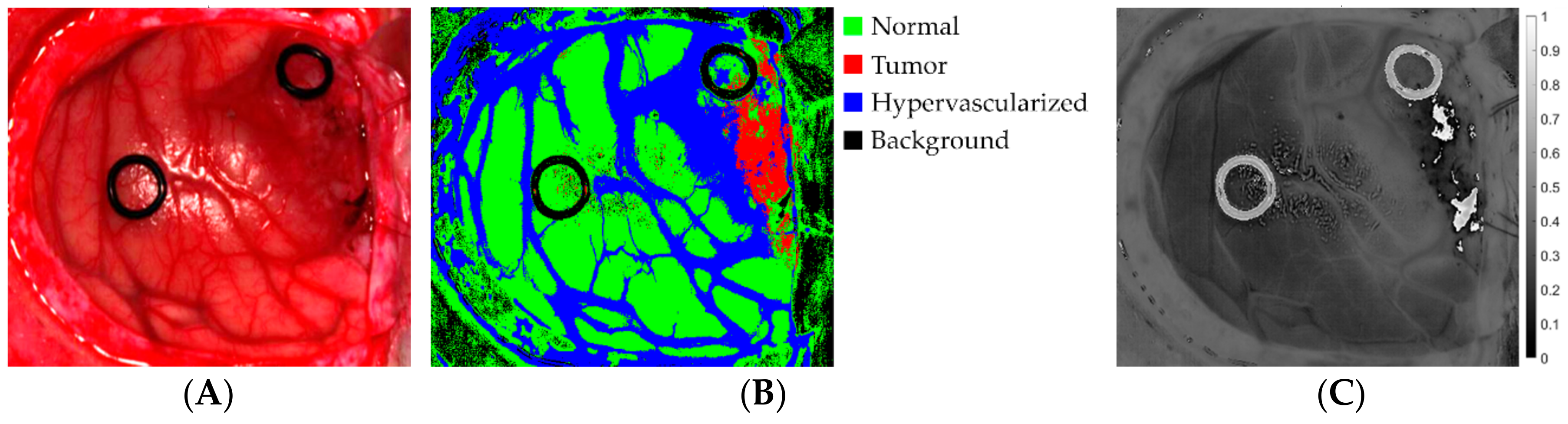
WSize2, the highest percentage is ~8.341%, considering the biggest image of the database, P1C2 (22,054 different pixels on 264,408). At this point, there is a further evaluation that can be made considering that this algorithm is part of a system whose main goal is to discriminate between tumor and healthy tissue. The classification is made between four classes that are normal tissue, tumor tissue, hypervascularized tissue and background [
22]. From the surgical and medical point of view, it is clear that a wrong discrimination between tumor and healthy tissue has much greater and transcendental relevance than just a misclassification issue between tumor and any other classes (hypervascularized and background) or between healthy, hypervascularized and background classes. It is possible to re-evaluate again the results of
Table 4, considering that, in the different
WSize executions, only a low percentage of different pixel labels are exchanged between tumor and normal tissue.
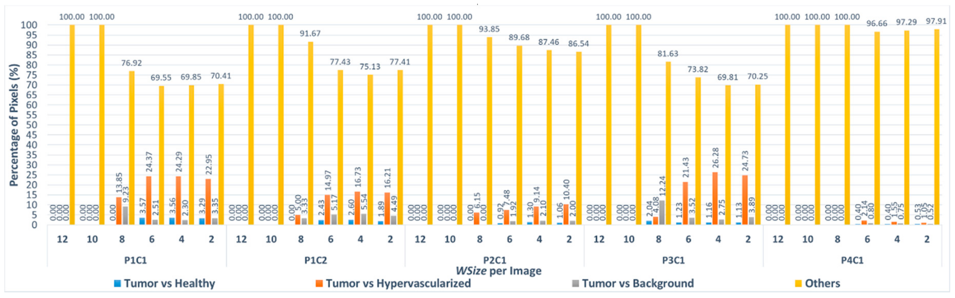
Figure 8 shows the percentage of pixels that are misclassified between tumor and healthy tissues, tumor and hypervascularized tissues and tumor and background, respectively, considering all the windows sizes for each image compared to the reference version. In addition, the graph presents the classification differences between healthy, hypervascularized and background classes (called
Others).
As it can be seen in
Figure 8, only in the case of the P3C1 image using the
WSize8, the algorithm misclassifies approximately 2% of the pixels (1 out of 49 pixels), exchanging the labels between tumor and healthy tissues. In all the other implementations of
WSize8, the classification differences do not involve the tumor class. Furthermore, in the versions related to the three smallest windows (
WSize6,
WSize4,
WSize2), the percentage of the pixels exchanged between these two classes is lower than the percentages of pixels exchanged between the other classes. For example, for the biggest image of the database (P1C2), in the
WSize6 implementation, the classification difference between tumor and healthy tissue represents 2.43% out of 2845 different pixels. Considering the same image in the
WSize4 and in the
WSize2 implementations, this percentage is 2.60% out of 7705 pixels and 1.89% out of 22,054 pixels, respectively. The highest percentage of differences between these two classes is found in the
WSize6 version regarding the P1C1 image, where it is around 3.57% out of 3672 pixels. According to these data, it is clear that the algorithm can correctly distinguish the tumor from the healthy tissue, while it makes more errors in separating the tumor from the hypervascularized tissue. The highest percentages of misclassified pixels between the tumor and the hypervascularized classes reach 26.28% of the total number of different pixels (P3C1 image,
WSize4 version). In fact, according to what it is said in [
22], these two classes referred to tissues with similar spectral signatures that can produce some misclassifications. On the other hand, the spectral signatures of tumor and healthy tissues present remarkable differences that allow the algorithm to distinguish these two classes in the classification.
4.2. KNN Window Search Optimization Results Using Manhattan Distance
As it was said before, the neighbors search represents the heaviest computational load of the KNN filtering algorithm. Although the distances computation is the most time-consuming task, the number of evaluated distances has been reduced in this study by considering a window, so a smallest area is considered instead of the entire image. To further reduce the execution time of this phase, the Manhattan metric has been tested instead of the Euclidean one, as described in Equation (3).
Table 5 compares the times of the serial code using both the entire image (
EI) and the reference window (
WSize14), applying both the Euclidean and the Manhattan distances. The speedup obtained using the Manhattan distance and the percentages of pixels that are different in the results are also presented in this table.
As said in the previous paragraph, searching the neighbors within a window instead of in the entire image allows saving time without changing the classification results. A further reduction of the execution time is obtained using the Manhattan metric in the distance computations. In fact, for the biggest image of the database (P1C2), the time is reduced from ~5 h (19,135.58 s) using the Euclidean distance to ~2 h (7683.44 s) in the case of using the entire image. If the neighbors are searched within the window (for the same image), the time decreases to ~3 min (202.42 s) using the Manhattan distance. Concerning all the images, it is possible to reach speedups from 2.22× to 3.33×, considering the versions with the entire image, and from 2.49× to 2.66× in the WSize14 executions. Comparing the implementations that exploit the Manhattan distance and the ones that use the Euclidean metric, the number of pixels classified with different labels is quite low: the highest percentage of different pixels is 1.33% in the P1C1 image. Furthermore, it is important to highlight that there are no differences in the classification results comparing the entire image and the WSize14 versions, using the Manhattan distance.
At this point, it is interesting to evaluate how the execution times can be reduced changing the size of the windows using the Manhattan metric in the distances computation. The results shown in
Table 6 confirm that decreasing the number of distance computations, i.e., the variations of the window sizes, allows further reductions of the computational time. The lowest execution times are obtained exploiting the GPU technology that can run the parallel algorithm taking ~8 s (compared to ~3 min) if the biggest image (P1C2) with the
WSize14 version is considered. The speedups obtained using this device and the optimizations introduced in the code are significant and they can reach up to 33.2× (P2C1-
WSize12). For some images and for some window dimensions, the algorithm takes only a few seconds, but what is even more important to consider is the number of pixels that are misclassified when the window size decreases (
Table 7).
As it can be seen in the results shown in
Table 7,
WSizes12 and
WSizes10 present a reduced number of different pixels compared to the other implementations. Analyzing the Euclidean distance results presented in
Table 4, this consideration can be made for the first three tests (
WSizes12,
WSizes10 and
WSize8) but, in this case, the number of different pixels in
WSize8 is higher than the first two versions. Despite this, it is important to highlight that the classification differences shown in
Table 7 are not very relevant for the final application of the system. In this application, a solution with a good compromise between real-time execution and classification accuracy of the results has to be selected. In addition, it is also important to evaluate the percentage of different pixels that are misclassified between tumor and healthy tissues and between tumor and the other classes.
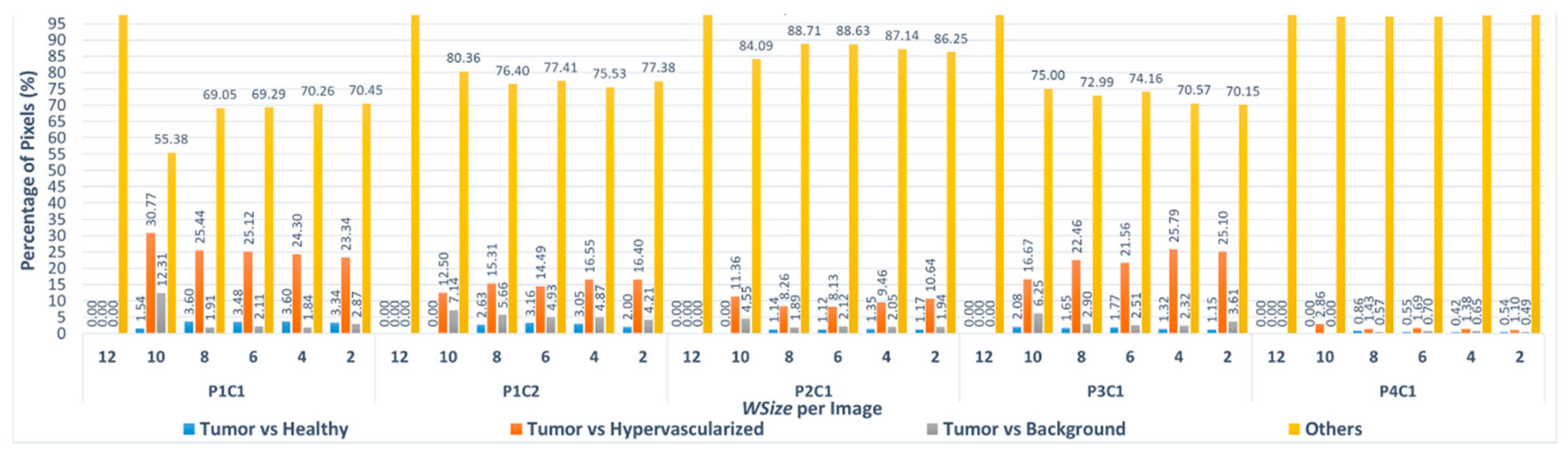
Figure 9 shows the percentage of pixels that are misclassified using the Manhattan metric between the different classes. In this figure, it is possible to notice that the algorithm misclassifies more pixels between tumor and hypervascularized classes than between tumor and healthy classes. In fact, the highest percentage of pixels misclassified is 30.77% related to the P1C1 image with
WSize10, where the algorithm exchanges the labels of 20 pixels (between tumor and hypervascularized tissue) out of a total amount of 65 different pixels compared to the reference version
WSize14 (
Table 7). Concerning the comparison between tumor and healthy classes, the number of pixels with an exchanged label is very low: the worst case is always the P1C1 image (
WSize8), where 66 out of 1832 different pixels are misclassified, being a 3.60% of pixels.
4.3. Summary
In this study, the results of serial and parallel versions of the KNN filtering algorithm for the classification of in-vivo brain tumor for hyperspectral images are introduced. In particular, the importance of reducing the area of the neighbors search in order to decrease the elaboration time is explained. In fact, the results prove that searching the neighbors of a pixel within a window instead of the entire image supposes a significant reduction of the computation time. It is important to notice that introducing a window (characterized by 14 rows with the reference pixel in the center) does not affect the result of the classification. For this reason, this version has been defined as the reference one (WSize14). Reducing the window size compared to the reference one, the time of the computation drastically decreases but the number of pixels that the algorithm misclassifies increases. At this point, it is important to select the best versions that have a good tradeoff between performance and number of misclassifications.
In the previous sections, the percentages and the number of different pixels between versions with different window sizes were analyzed. Concerning the implementations that exploit the Euclidean distance,
Table 4 demonstrated that by using the window sizes
WSize12,
WSize10 and
WSize8, the number of different pixels was lower than those obtained using the
WSize6,
WSize4 and
WSize2, compared with the reference test (
WSize14).
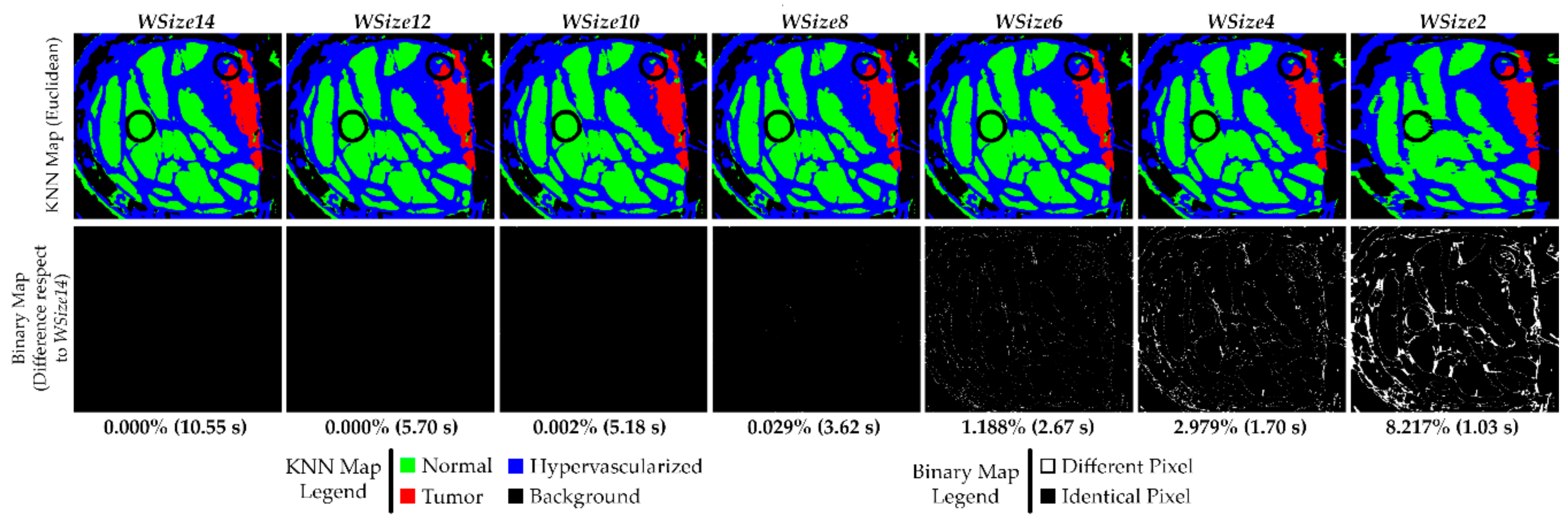
In
Figure 10, the KNN filtered maps obtained from the P2C1 image and the binary maps are shown, where the differences between the evaluated window size version and the reference version are highlighted. Despite the differences between the first and the last three versions shown in
Table 4, it is possible to see that the KNN filtered maps of the implementations for
WSize6 and
WSize8 do not present relevant dissimilarities. In fact, it is important to remember that the main goal of these maps is to delineate the tumor area, in order to provide the surgeons with a guidance tool during the tumor resection. In this context, it is clear that the number of different pixels in
WSize8 and
WSize6 versions are not so significant for the final application of the system, since the surgeon always resect a security margin around the tumor tissue.
In the previous paragraph, the data showed that the algorithm is able to correctly discriminate between tumor and healthy classes. This consideration can also be seen in the KNN filtered maps, where the area related to the tumor tissue (red) remains roughly the same in the implementations WSize6, WSize8, WSize10 and WSize12 compared to the WSize14 one. Considering the WSize4 and the WSize2 versions, it is possible to appreciate that the margins of the tumor are not as evident and well defined as in the other images, confirming what has been said in the previous paragraphs while analyzing the classification results.
The second row of
Figure 10 presents the binary maps that show the pixel differences between all the window size versions and the reference implementation (
WSize14). In particular, by analyzing the binary maps of
WSize4 and
WSize2, it is possible to identify several differences compared to
WSize14. For this reason, these two versions should not be chosen for the final solution. However, in the binary maps of
WSize6 and
WSize8, there are few differences, and they are barely appreciated analyzing the KNN filtered maps. It is important to remember that the suitable version for this application is the option that offers a good compromise between accurate classification and fast execution. Exploiting the GPU technology, the parallel version of the KNN algorithm with
WSize8 takes ~3.62 s to filter the P2C1 image, while the
WSize6 implementation is executed in ~2.67 s. For the biggest image of the database (P1C2), the
WSize6 implementation allows to save ~2 s when compared to the
WSize8 version. According to these results, the
WSize8 version has been selected as the best solution, giving priority to the classification accuracy but considering also a fast implementation. On the contrary, the
WSize6 implementation has been chosen as the fastest implementation with acceptable accuracy results.
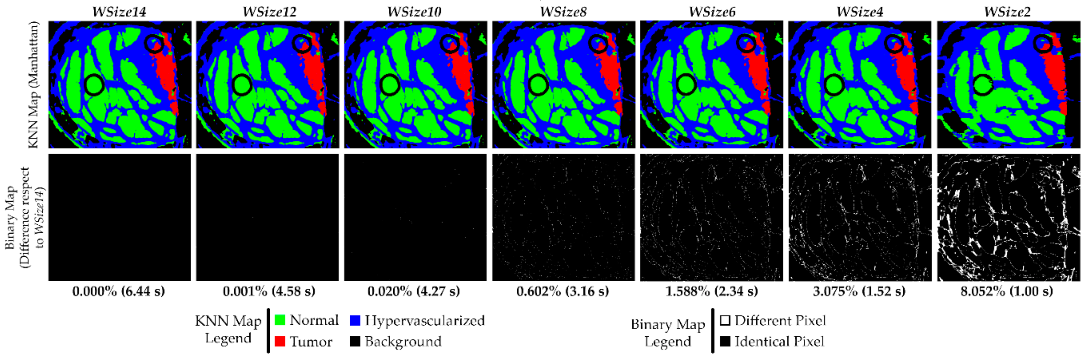
Similarly, the same evaluation can be done considering the implementations that exploit the Manhattan metric for the computation of the distances. Analyzing the computational times in the previous sections, it is evident that this metric leads to faster executions than the Euclidean distance. The first row of
Figure 11 shows the KNN filtered maps of the P2C1 image using different window sizes and using the Manhattan distance. The second row presents the binary maps to evaluate the differences between the developed versions when compared to the
WSize14 implementation. According to the data shown in
Table 7, in
Figure 11 it is possible to see that the KNN filtered maps of the versions
WSize12 and
WSize10 are practically identical to the map obtained with
WSize14. The number of different pixels is low enough to not perceive the differences between the classification maps. In
Table 7, it is also evident that the number of different pixels from the
WSize8 to the
WSize2 implementations drastically increases. Concerning the KNN filtered maps of the
WSize4 and, in particular, the
WSize2 implementations, the differences are very clear since the margin of the tumor is not as well defined as in the other maps. Instead, in the filtered maps of the
WSize8 and
WSize6 implementations, the classification differences are not so evident, especially taking into account the tumor tissue area. The differences between all the versions compared to the
WSize14 implementation can be evaluated in the binary maps (
Figure 11, second row). Even if the
WSize4 and
WSize2 are the fastest implementations, their binary maps clearly show that these two versions cannot be chosen because the amount of different pixels compared to
WSize14 is too high. However, in the binary maps of
WSize12 and
WSize10, it is evident that these implementations offer the highest accuracy but the slowest execution times. Finally, concerning the
WSize8 and
WSize6 implementations, it is possible to determine that the
WSize8 version has the highest accuracy but the execution time is slower than the
WSize6 version (the former exhibits 3.16 s and the latter 2.34 s). Also in this case, the best solution is chosen on the basis of the degree of accuracy and the time constraints that the application requires.
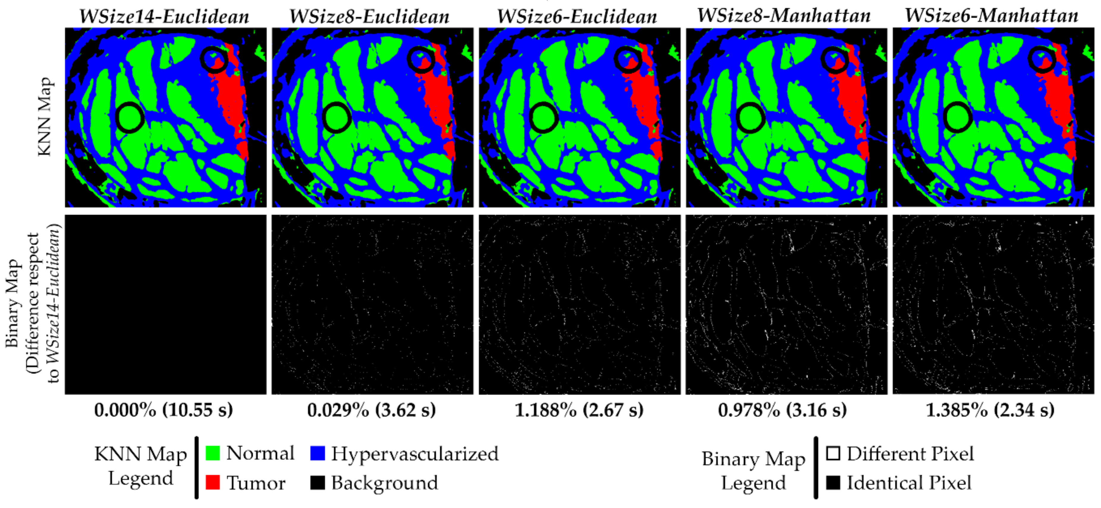
At this point, the best solutions selected between the Manhattan versions (WSize8 and WSize6) have to be compared with the reference test WSize14 that exploits the Euclidean distance. The original algorithm is characterized by the use of the Euclidean metric in the neighbors search within the entire image. Since the WSize14 Euclidean implementation does not have any differences in the classification results compared to the original version, the results of the Manhattan best solutions have to be compared with the reference results.
By analyzing the results comparison shown in
Figure 12, it is possible to see that all these versions have a reduced percentage of different pixels compared to the
WSize14-Euclidean implementation. In all the obtained KNN filtered maps, the boundaries of the tumor area are accurately defined.
The solutions where the results are more similar to the reference implementation are the
WSize8-Euclidean and
WSize8-Manhattan versions, which differ 0.029% and 0.978% respectively, compared to the
WSize14-Euclidean reference. The versions characterized by a window with 6 rows are less accurate than the previous ones, but they are faster. Concerning the computational times, the parallel execution of the reference solution is executed in ~10.55 s, while the
WSize8-Euclidean and
WSize8-Manhattan versions are executed in 3.62 and 3.16 s, respectively. The
WSize6-Euclidean and
WSize6-Manhattan implementations require 2.67 and 2.34 s, respectively. Finally, a figure of merit (
FoM in Equation (5)), which relates the execution time (
t) and the classification results (
err), was considered to select the best solution that offers the highest value. The version
WSize8-Euclidean is chosen as the best solution since it presents the highest value of
FoM (
Figure 13). To the best of our knowledge, the state of the art does not provide implementations of the KNN filtering algorithm that could be a touchstone for a fair comparison with the presented work.


 ,
, 


