Evaluation of the Accuracy of Bathymetry on the Nearshore Coastlines of Western Korea from Satellite Altimetry, Multi-Beam, and Airborne Bathymetric LiDAR


Abstract
:1. Introduction
2. Data sets and Methodology
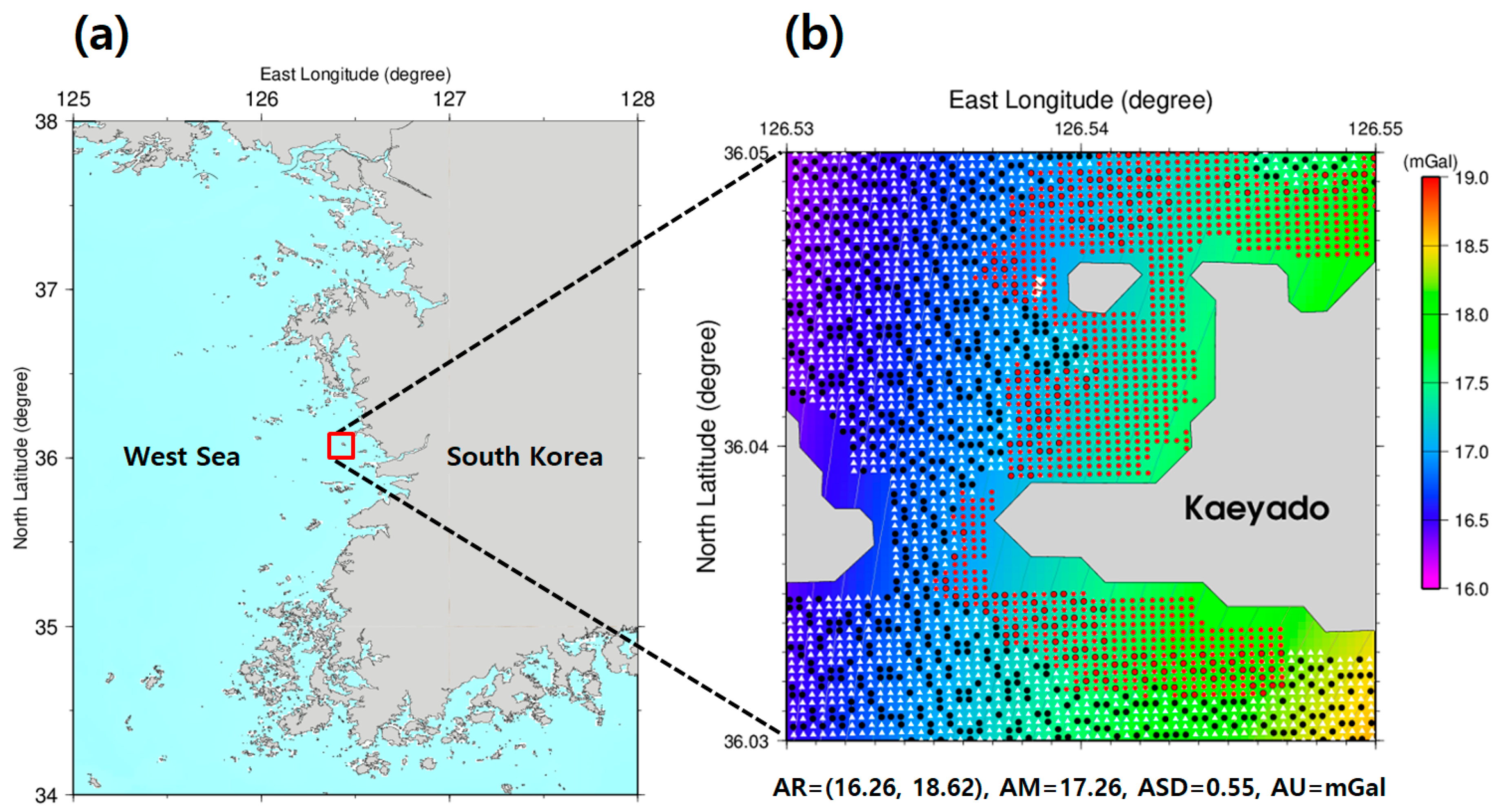
2.1. Study Area
2.2. Data Set
2.2.1. Multi-Beam
2.2.2. Bathymetric LiDAR
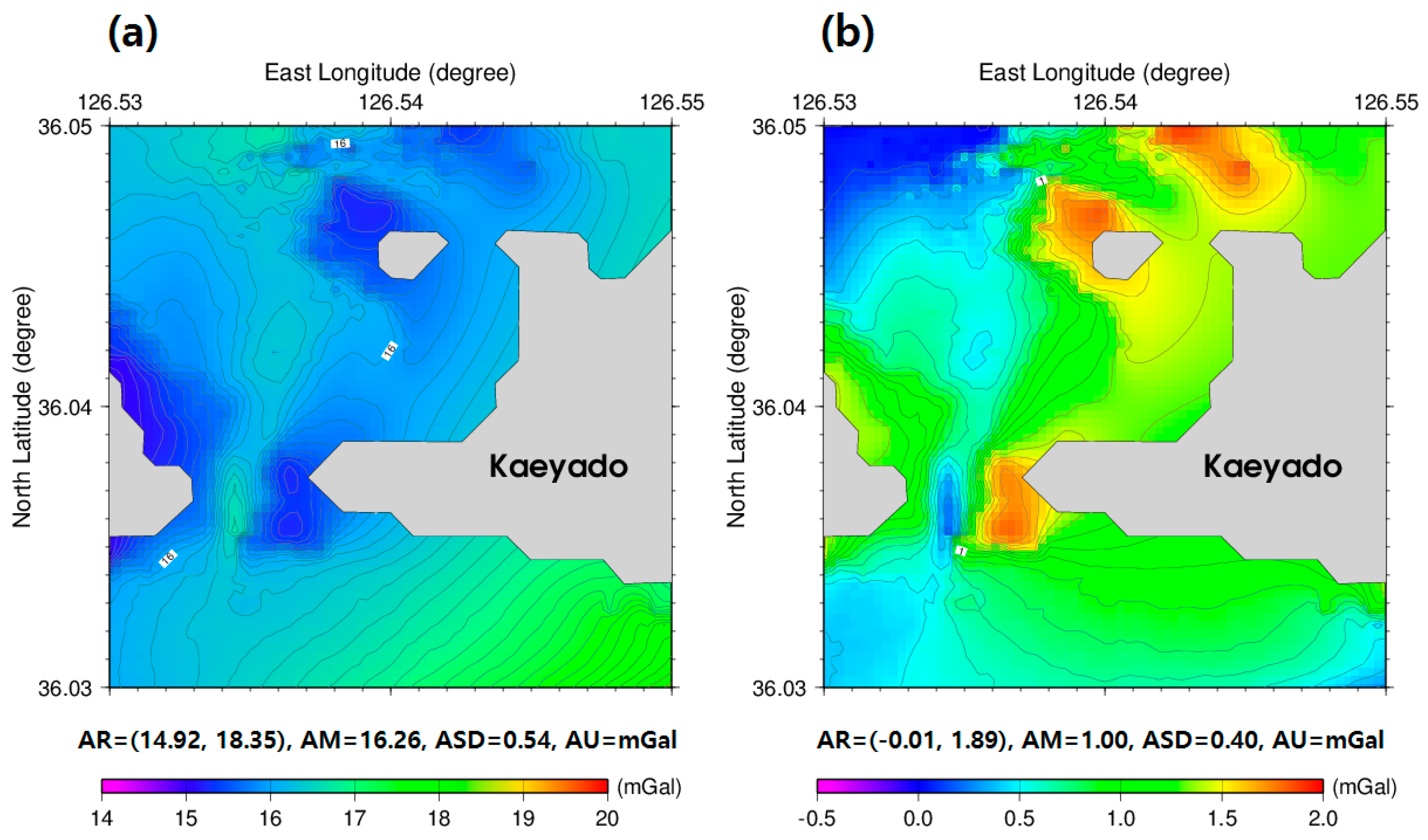
2.2.3. Satellite Altimetry-Derived Gravity Anomaly
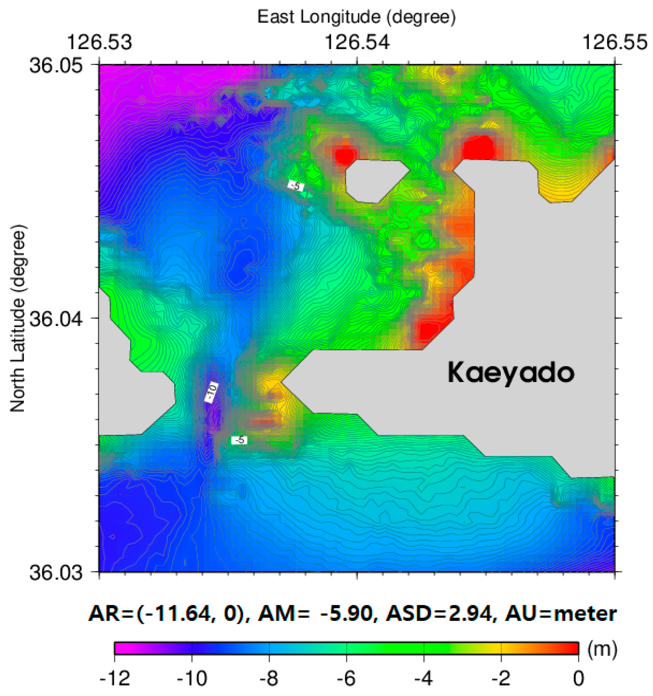
2.3. Methodology
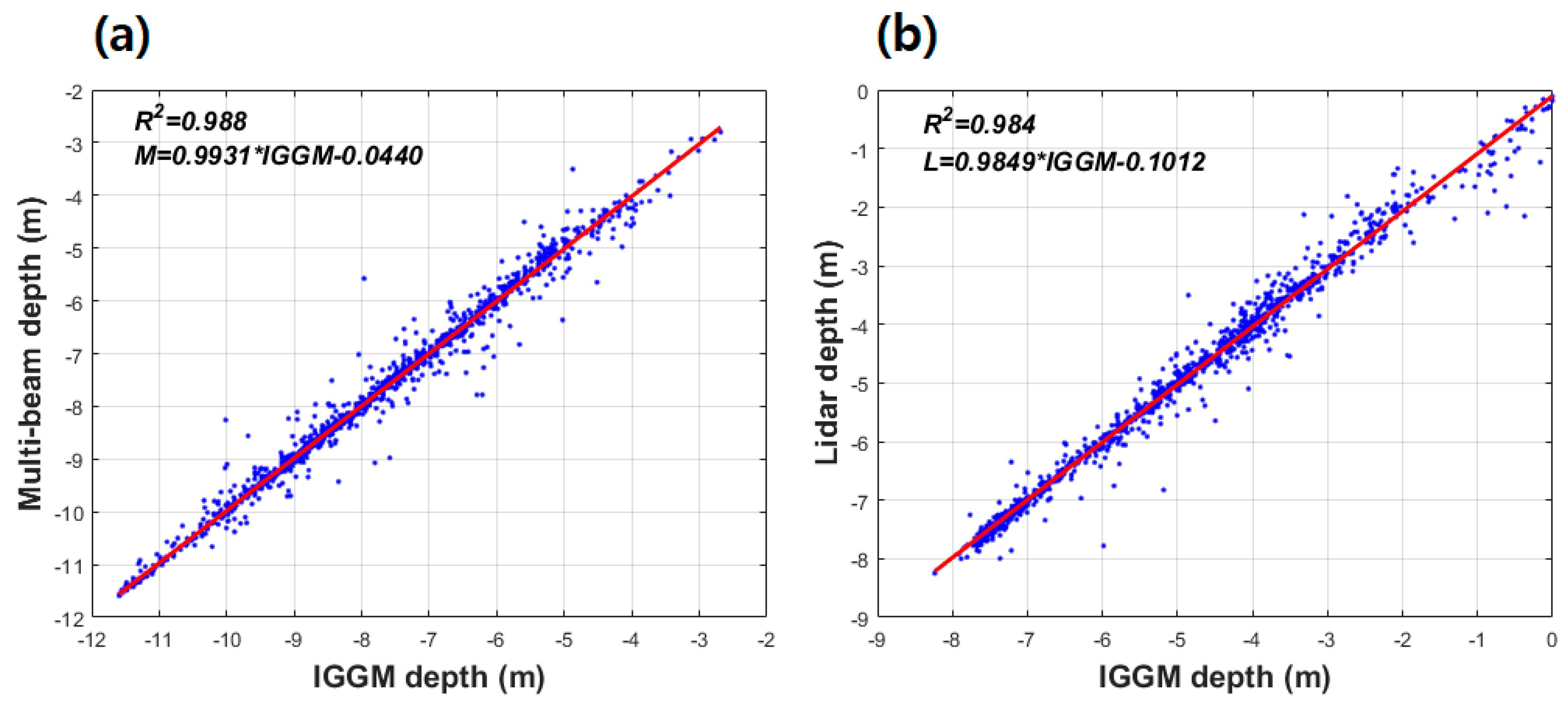
3. Results
4. Discussion
5. Conclusions
Author Contributions
Funding
Acknowledgments
Conflicts of Interest
References
- Stafford, D.B.; Langfelder, J. Air photo survey of coastal erosion. Photogramm. Eng. 1971, 37, 565–575. [Google Scholar]
- Moore, L.J.; Benumof, B.T.; Griggs, G.B. Coastal erosion hazards in Santa Cruz and San Diego Counties, California. J. Coastal Res. 1999, SI28, 121–139. [Google Scholar]
- Battiau-Queney, Y.; Billet, J.F.; Chaverot, S.; Lanoy-Ratel, P. Recent shoreline mobility and geomorphologic evolution of macrotidal sandy beaches in the north of France. Mar. Geol. 2003, 194, 31–45. [Google Scholar] [CrossRef]
- Aiello, A.; Canora, F.; Pasquariello, G.; Spilotro, G. Shoreline variations and coastal dynamics: A space–time data analysis of the Jonian littoral, Italy. Estuar. Coast. Shelf Sci. 2013, 129, 124–135. [Google Scholar] [CrossRef]
- Alesheikh, A.A.; Ghorbanali, A.; Nouri, N. Coastline change detection using remote sensing. Int. J. Environ. Sci. Technol. 2007, 4, 61–66. [Google Scholar] [CrossRef] [Green Version]
- Sunder, S.; Ramsankaran, R.A.A.J.; Ramakrishnan, B. Inter-comparison of remote sensing sensing-based shoreline mapping techniques at different coastal stretches of India. Environ. Monit. Assess. 2017, 189, 290. [Google Scholar] [CrossRef] [PubMed]
- Niedermeier, A.; Romaneessen, E.; Lehner, S. Detection of coastlines in SAR images using wavelet methods. IEEE Trans. Geosci. Remote Sens. 2000, 38, 2270–2281. [Google Scholar] [CrossRef]
- Demir, N.; Oy, S.; Erdem, F.; Seker, D.Z.; Bayram, B. Integrated shoreline extraction approach with use of Rasat MS and SENTINEL-1A SAR Images. ISPRS Annals of Photogramm. Remote Sens. Spa. Inf. Sci. 2017, 445–449. [Google Scholar] [CrossRef]
- White, S.A.; Wang, Y. Utilizing DEMs derived from LIDAR data to analyze morphologic change in the North Carolina coastline. Remote Sens. Environ. 2003, 85, 39–47. [Google Scholar] [CrossRef]
- Deronde, B.; Houthuys, R.; Henriet, J.P.; Lancker, V.V. Monitoring of the sediment dynamics along a sandy shoreline by means of airborne hyperspectral remote sensing and LIDAR: A case study in Belgium. Earth Surf. Proc. Land. 2008, 33, 280–294. [Google Scholar] [CrossRef]
- Templin, T.; Popielarczyk, D.; Kosecki, R. Application of low-cost fixed-wing UAV for inland lakes shoreline investigation. Pure Appl. Geophys. 2017, 1–21. [Google Scholar] [CrossRef]
- Topouzelis, K.; Papakonstantinou, A.; Doukari, M. Coastline change detection using Unmanned Aerial Vehicles and image processing technique. Fresen. Environ. Bull. 2017, 26, 5564–5571. [Google Scholar]
- Plant, N.G.; Holman, R.A. Intertidal beach profile estimation using video images. Mar. Geol. 1997, 140, 1–24. [Google Scholar] [CrossRef]
- Guedes, R.M.; Calliari, L.J.; Holland, K.T.; Plant, N.G.; Pereira, P.S.; Alves, F.N. Short-term sandbar variability based on video imagery: comparison between time–average and time–variance techniques. Mar. Geol. 2011, 289, 122–134. [Google Scholar] [CrossRef]
- De Moustier, C.; Matsumoto, H. Seafloor acoustic remote sensing with multibeam echo-sounders and bathymetric sidescan sonar systems. Mar. Geophys. Res. 1993, 15, 27–42. [Google Scholar] [CrossRef] [Green Version]
- Hughes Clarke, J.E.; Mayer, L.A.; Wells, D.E. Shallow-water imaging multibeam sonars: A new tool for investigating seafloor processes in the coastal zone and on the continental shelf. Mar. Geophys. Res. 1996, 18, 607–629. [Google Scholar] [CrossRef]
- Canepa, G.; Pace, N.G. Seafloor segmentation from multibeam bathymetric sonar. In Proceedings of the Fifth European Conference on Underwater Acoustics, Lyon, France, 10–13 July 2000; pp. 361–366. [Google Scholar]
- Atallah, L.; Smith, P.J.P.; Bates, C.R. Wavelet analysis of bathymetric sidescan sonar data for the classification of seafloor sediments in Hopvågen Bay-Norway. Mar. Geophys. Res. 2002, 23, 431–442. [Google Scholar] [CrossRef]
- Ibrahim, A.; Hinze, W.J. Mapping Buried Bedrock Topography with Gravity. Ground Water. 1972, 10, 18–23. [Google Scholar] [CrossRef]
- Kim, K.B.; Hsiao, Y.-S.; Kim, J.W.; Lee, B.Y.; Kwon, Y.K.; Kim, C.H. Bathymetry enhancement by altimetry-derived gravity anomalies in the East Sea (Sea of Japan). Mar. Geophys. Res. 2010, 31, 285–298. [Google Scholar] [CrossRef]
- Hsiao, Y.-S.; Kim, J.W.; Kim, K.B.; Lee, B.Y.; Hwang, C. Bathymetry estimation by gravity-geologic method: Investigation of density contrast predicted by downward continuation. Terr. Atmos. Ocean. Sci. 2011, 22, 347–358. [Google Scholar] [CrossRef]
- Kim, J.W.; von Frese, R.R.B.; Lee, B.Y.; Roman, D.R.; Doh, S.J. Altimetry-derived gravity predictions of bathymetry by gravity-geologic method. Pure Appl. Geophys. 2011, 168, 815–826. [Google Scholar] [CrossRef]
- Kim, K.B.; Lee, C.K. Bathymetry change investigation of the 2011 Tohoku earthquake. J. Kor. Soc. Surv. Geodesy Photogramm. Cartogr. 2015, 33, 181–192. [Google Scholar] [CrossRef]
- Hsiao, Y.-S.; Hwang, C.; Cheng, Y.-S.; Chen, L.-C.; Hsu, H.-J.; Tsai, J.-H.; Liu, C.-L.; Wang, C.-C.; Liu, Y.-C.; Kao, Y.-C. High-resolution depth and coastline over major atolls of South China Sea from satellite altimetry and imagery. Remote Sens. Environ. 2016, 176, 69–83. [Google Scholar] [CrossRef]
- Kim, K.B.; Yun, H.S. Satellite-derived Bathymetry Prediction in Shallow Waters Using the Gravity-Geologic Method: A Case Study in the West Sea of Korea. KSCE J. Civ. Eng. 2018, 22, 2560–2568. [Google Scholar] [CrossRef]
- Aarninkhof, S.G.J.; Turner, I.L.; Dronkers, T.D.T.; Caljouw, M.; Nipius, L. A video-based technique for mapping intertidal beach bathymetry. Coast. Eng. 2003, 49, 275–289. [Google Scholar] [CrossRef]
- Bergsma, E.W.J.; Conley, D.C.; Davidson, M.A.; O’Hare, T.J. Video-based nearshore bathymetry estimation in macro-tidal environments. Mar. Geol. 2016, 374, 31–41. [Google Scholar] [CrossRef]
- Osorio, A.F.; Medina, R.; Gonzalez, M. An algorithm for the measurement of shoreline and intertidal beach profiles using video imagery: PSDM. Comput. Geosci. 2012, 46, 196–207. [Google Scholar] [CrossRef]
- Uunk, L.; Wijnberg, K.M.; Morelissen, R. Automated mapping of the intertidal beach bathymetry from video images. Coast. Eng. 2010, 57, 461–469. [Google Scholar] [CrossRef]
- Wang, C.K.; Philpot, W.D. Using airborne bathymetric lidar to detect bottom type variation in shallow waters. Remote Sens. Environ. 2007, 106, 123–135. [Google Scholar] [CrossRef]
- Brock, J.C.; Purkis, S.J. The emerging role of lidar remote sensing in coastal research and resource management. J. Coastal Res. 2009, SI53, 1–5. [Google Scholar] [CrossRef]
- Irish, J.L.; McClung, J.K.; Lillycrop, W.J. Airborne Lidar Bathymetry: The SHOALS System; U.S. Army Corps of Engineer, Mobile District: Mobile, AL, USA, 2016. [Google Scholar]
- Eisemann, E.R.; Wallace, D.J.; Buijsman, M.C.; Pierce, T. Response of a vulnerable barrier island to multi-year storm impacts: LiDAR-data-inferred morphodynamic changes on Ship Island, Mississippi, USA. Geomorphology 2018, 313, 58–71. [Google Scholar] [CrossRef]
- Sandwell, D.T.; Smith, W.H.F. Global marine gravity from retracked Geosat and ERS-1 altimetry: Ridge segmentation versus spreading rate. J. Geophys. Res. 2009, 114, B01411. [Google Scholar] [CrossRef]
- Teledyne Marine. Available online: http://www.teledynemarine.com/ (accessed on 24 July 2018).
- Teledyne Optech. Available online: http://www.teledyneoptech.com/ (accessed on 24 July 2018).
- Sandwell, D.T.; Garcia, E.; Soofi, K.; Wessel, P.; Chandler, M.; Smith, W.H.F. Toward 1-mGal accuracy in global marine gravity from CryoSat-2, Envisat, and Jason-1. Lead. Edge 2013, 32, 892–899. [Google Scholar] [CrossRef]
- Guenther, G.C. Airborne lidar bathymetry. In Digital Elevation Model Technologies and Applications: The DEM Users Manual, 2nd ed.; American Society for Photogrammetry and Remote Sensing: Bethesda, MD, USA, 2007; pp. 253–320. [Google Scholar]
- Wessel, P.; Smith, W.H.F.; Scharroo, R.; Luis, J.; Wobbe, F. Generic Mapping Tools: Improved version released. EOS Trans. Am. Geophys. Union 2013, 94, 409–410. [Google Scholar] [CrossRef]


| Type | Multi-Beam Bathymetry | Airborne Bathymetric LiDAR | Satellite Altimetry-Derived Gravity Anomalies |
|---|---|---|---|
| Sensor | Seabat 7125 | CZMIL | Altimeter |
| Platform | shipborne | airborne | spaceborne |
| Ellipsoid | WGS-84 | WGS-84 | WGS-84 |
| Unit | meter | meter | mGal |
| Reference surface | Datum Level | Datum Level | Mean Sea Level |
| Min. | Max. | Mean | Std. Dev. | RMSE | |
|---|---|---|---|---|---|
| GGM–KHOA | 0.00 | 2.44 | 0.08 | 0.18 | 0.19 |
| GGM–LiDAR | 0.00 | 5.49 | 0.65 | 0.93 | 1.13 |
| Min. | Max. | Mean | Std. Dev. | RMSE | |
|---|---|---|---|---|---|
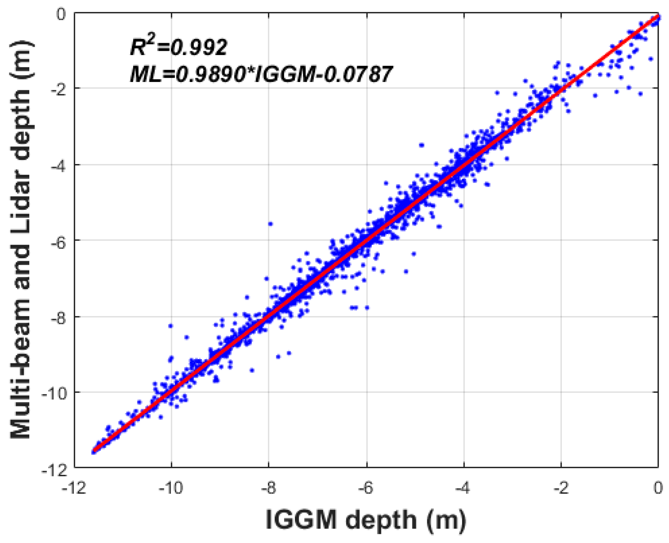
| IGGM–KHOA | 0.00 | 2.39 | 0.08 | 0.16 | 0.18 |
| IGGM–LiDAR | 0.00 | 1.80 | 0.14 | 0.19 | 0.24 |
| Min. | Max. | Mean | Std. Dev. | RMSE | |
|---|---|---|---|---|---|
| IGGM − (KHOA + LiDAR) | 0.00 | 2.39 | 0.10 | 0.18 | 0.20 |
© 2018 by the authors. Licensee MDPI, Basel, Switzerland. This article is an open access article distributed under the terms and conditions of the Creative Commons Attribution (CC BY) license (http://creativecommons.org/licenses/by/4.0/).
Share and Cite
Yeu, Y.; Yee, J.-J.; Yun, H.S.; Kim, K.B. Evaluation of the Accuracy of Bathymetry on the Nearshore Coastlines of Western Korea from Satellite Altimetry, Multi-Beam, and Airborne Bathymetric LiDAR. Sensors 2018, 18, 2926. https://0-doi-org.brum.beds.ac.uk/10.3390/s18092926
Yeu Y, Yee J-J, Yun HS, Kim KB. Evaluation of the Accuracy of Bathymetry on the Nearshore Coastlines of Western Korea from Satellite Altimetry, Multi-Beam, and Airborne Bathymetric LiDAR. Sensors. 2018; 18(9):2926. https://0-doi-org.brum.beds.ac.uk/10.3390/s18092926
Chicago/Turabian StyleYeu, Yeon, Jurng-Jae Yee, Hong Sik Yun, and Kwang Bae Kim. 2018. "Evaluation of the Accuracy of Bathymetry on the Nearshore Coastlines of Western Korea from Satellite Altimetry, Multi-Beam, and Airborne Bathymetric LiDAR" Sensors 18, no. 9: 2926. https://0-doi-org.brum.beds.ac.uk/10.3390/s18092926