Collective Anomalies Detection for Sensing Series of Spacecraft Telemetry with the Fusion of Probability Prediction and Markov Chain Model

Abstract
:1. Introduction
2. Related Works
3. Anomaly Detection with Probability Prediction Models
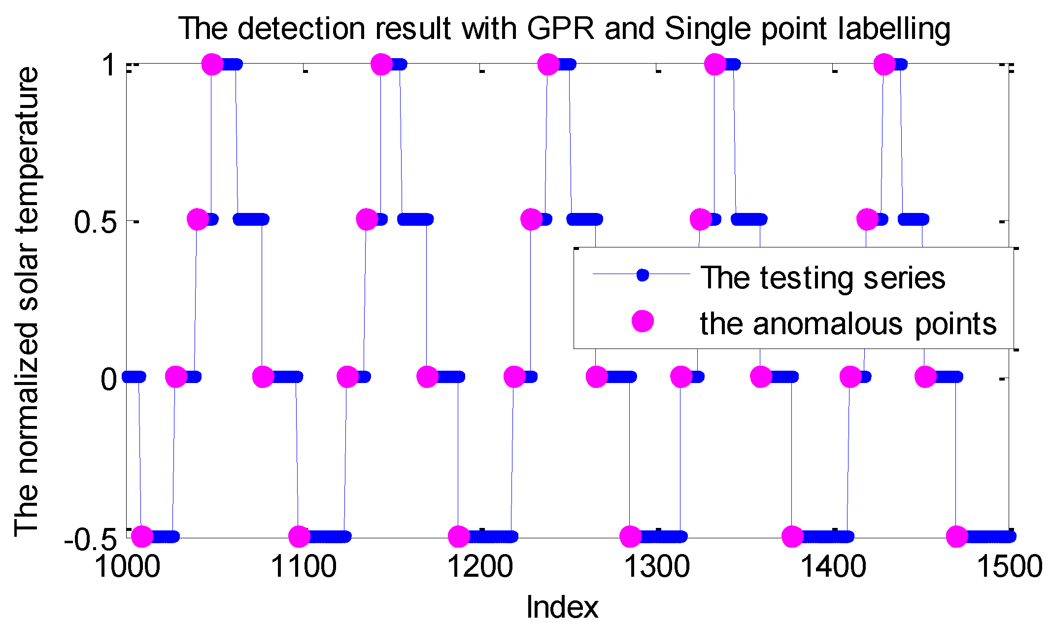
3.1. Probability Prediction with the Gaussian Process Regression Model
3.2. Probability Prediction with the Relevance Vector Machine Model
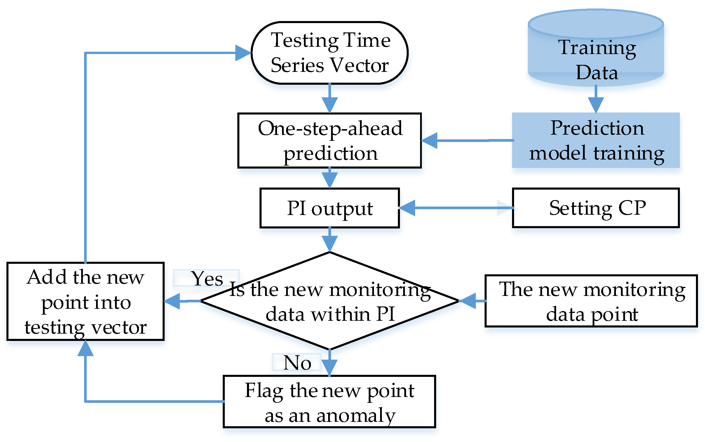
3.3. Anomaly Detection with Prediction Interval Constructed by Probability Prediction Model
3.4. Problem Formulation
4. Markov Chain Labelling Fused with Probability Prediction-Based Method
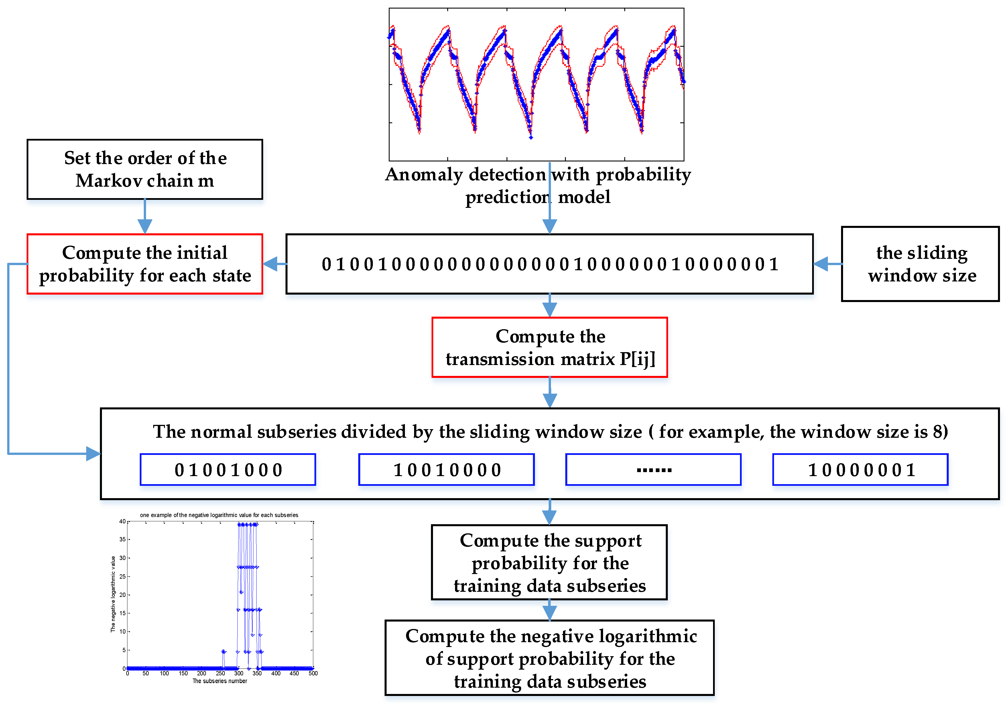
4.1. Markov Chain Model
4.2. Markov Chain Training for Normal Series Labeled by the Probability Prediction Model
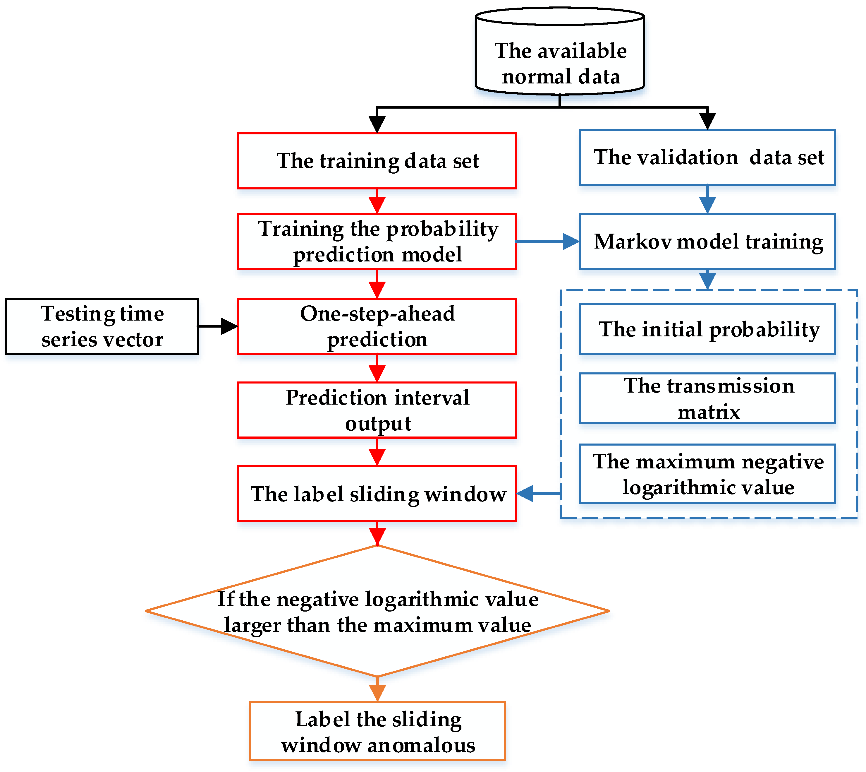
4.3. Anomaly Detection with Markov Chain Fused with Probability Prediction-Based Method
5. Experimental Results and Analysis
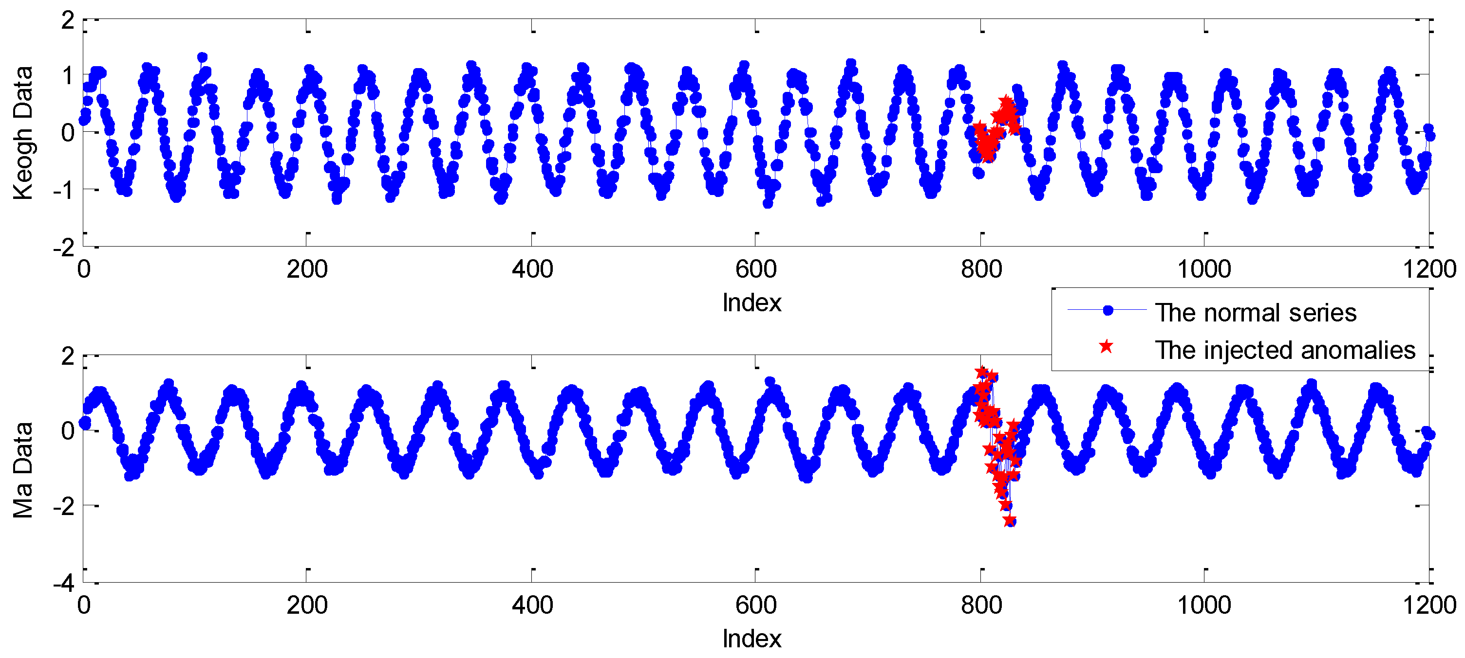
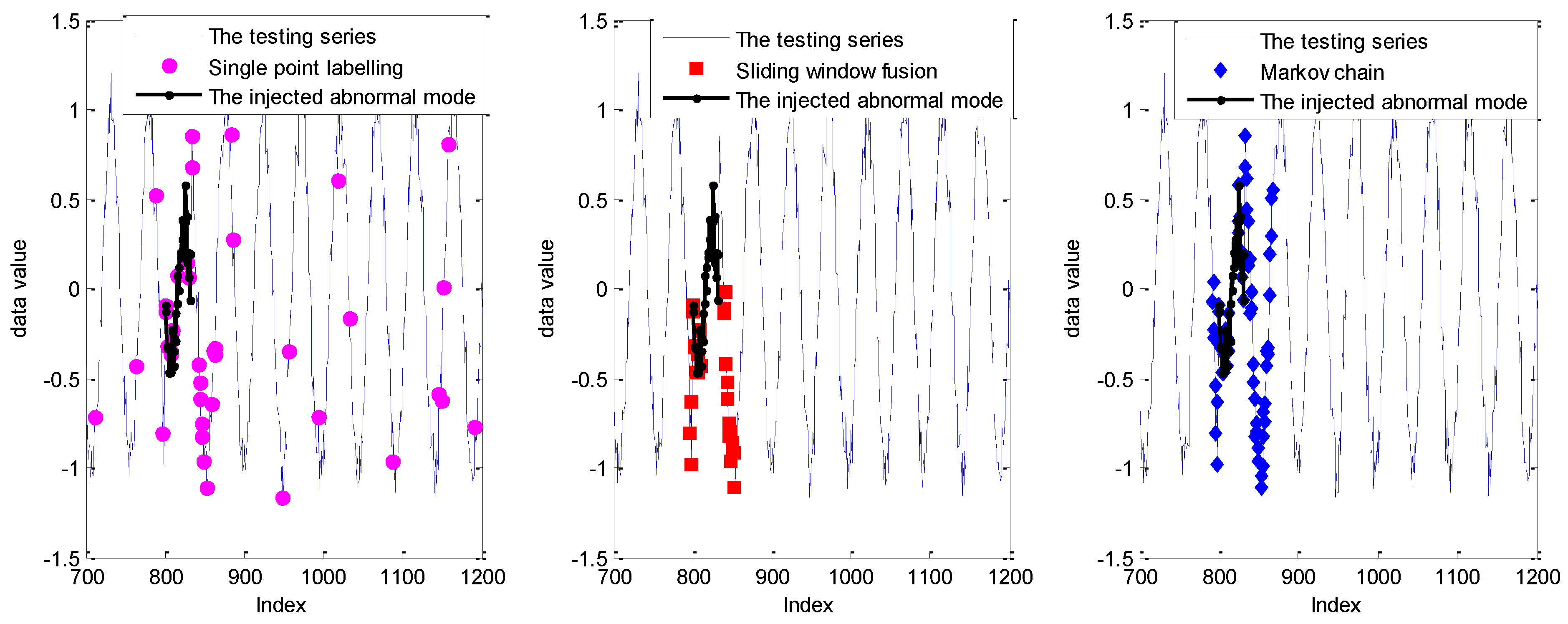
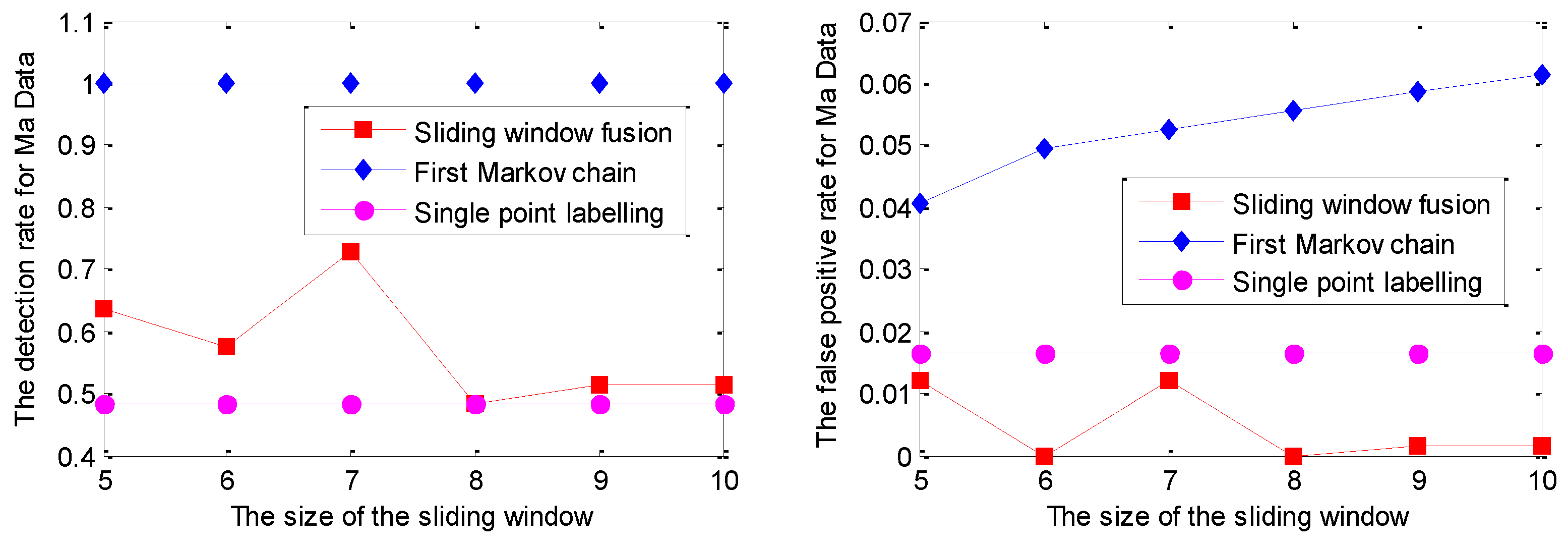
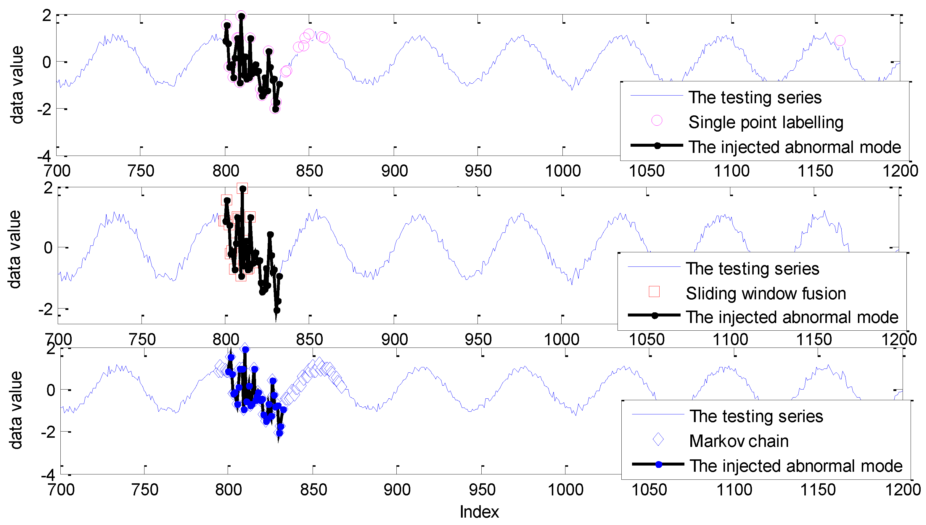
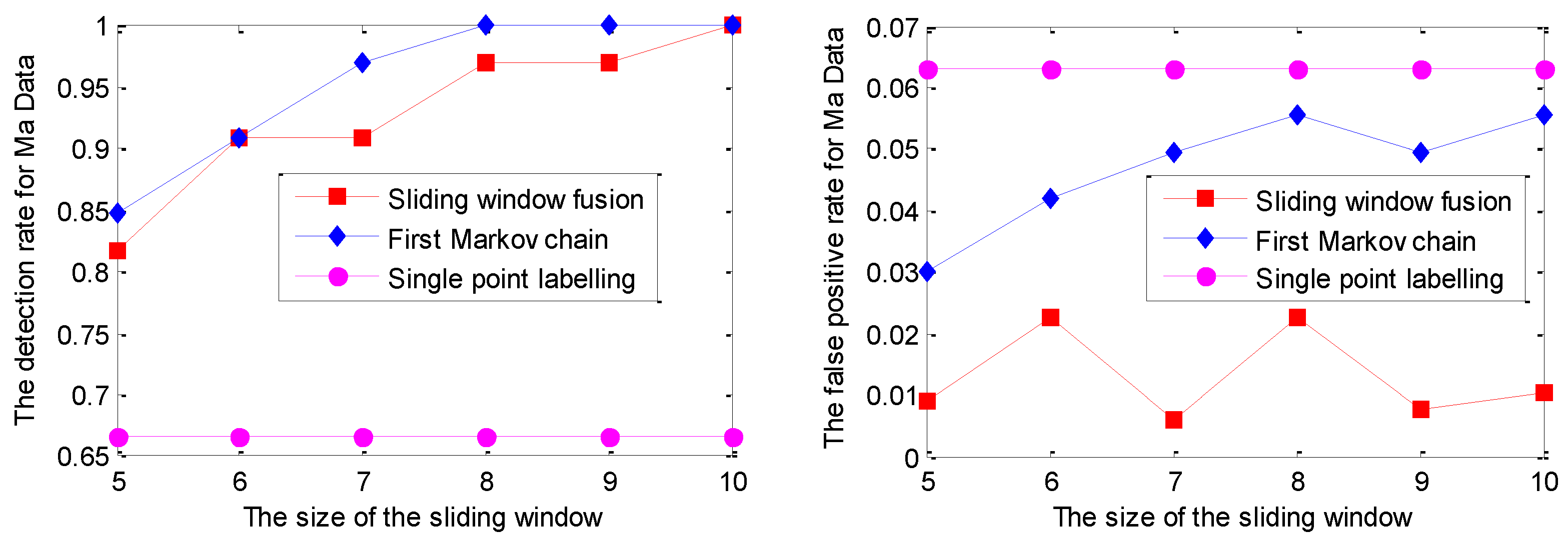
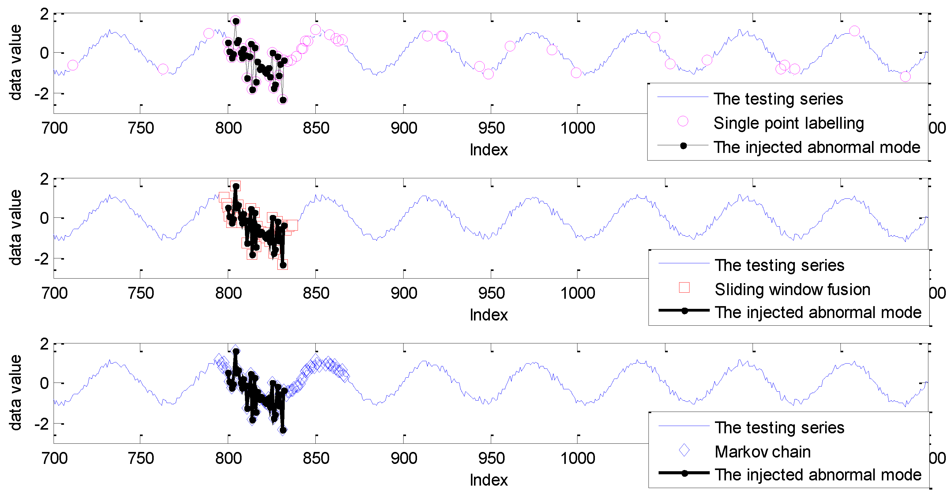
5.1. Experiments on Simulated Data Sets
5.2. Experiments on Normal Telemetry Series
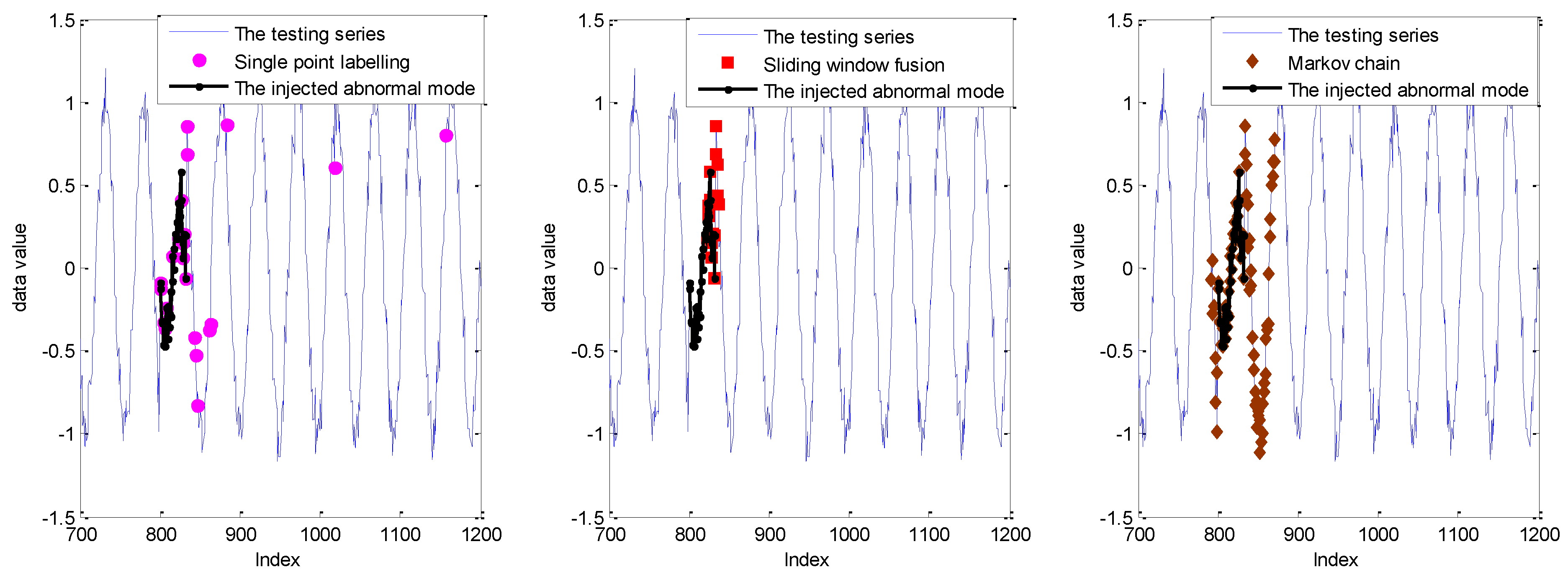
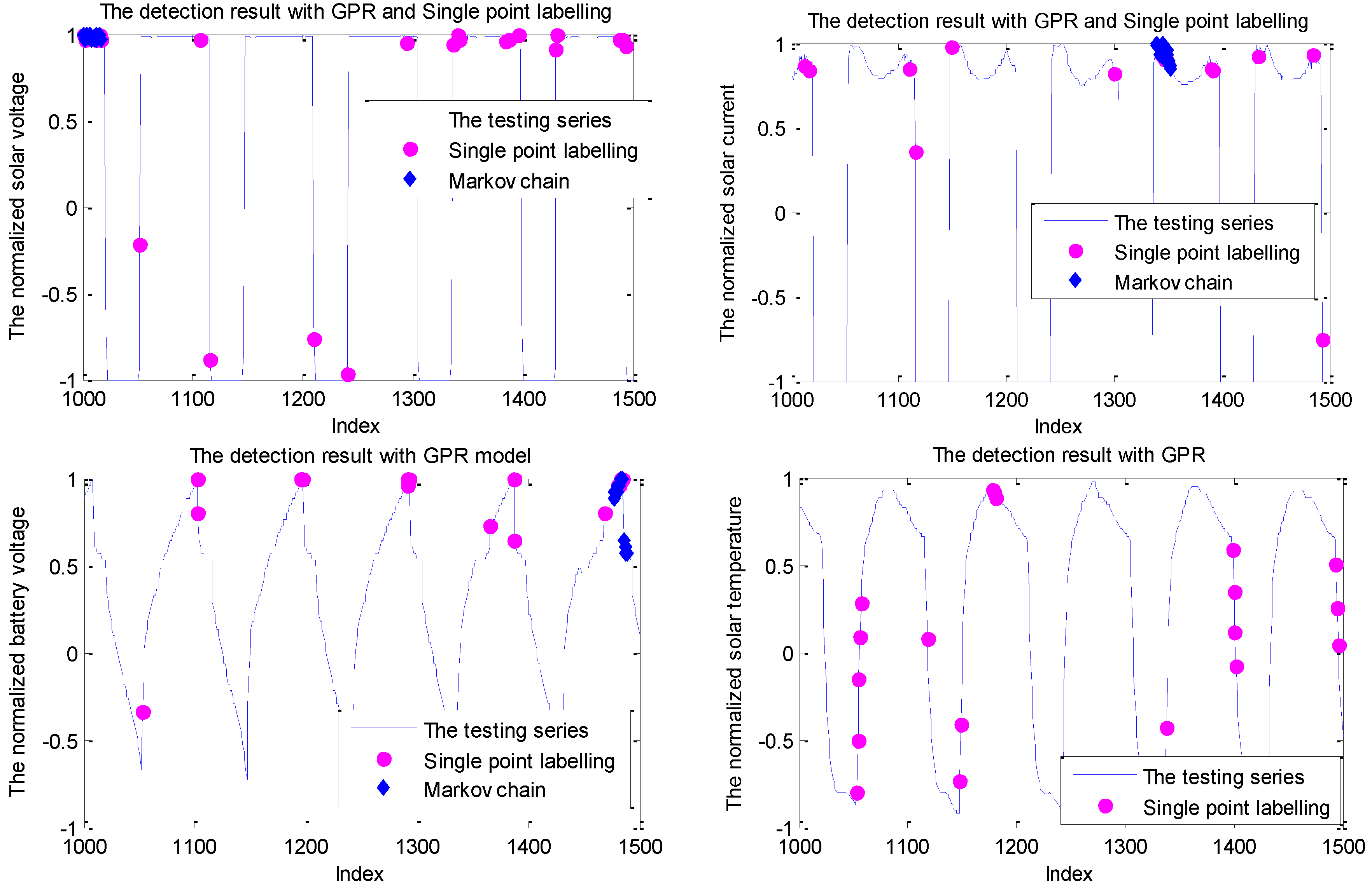
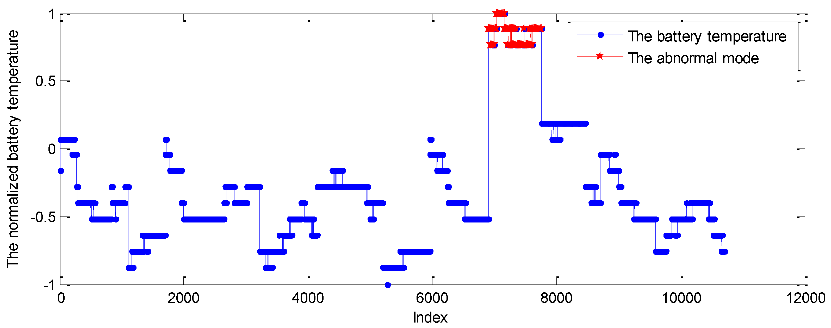
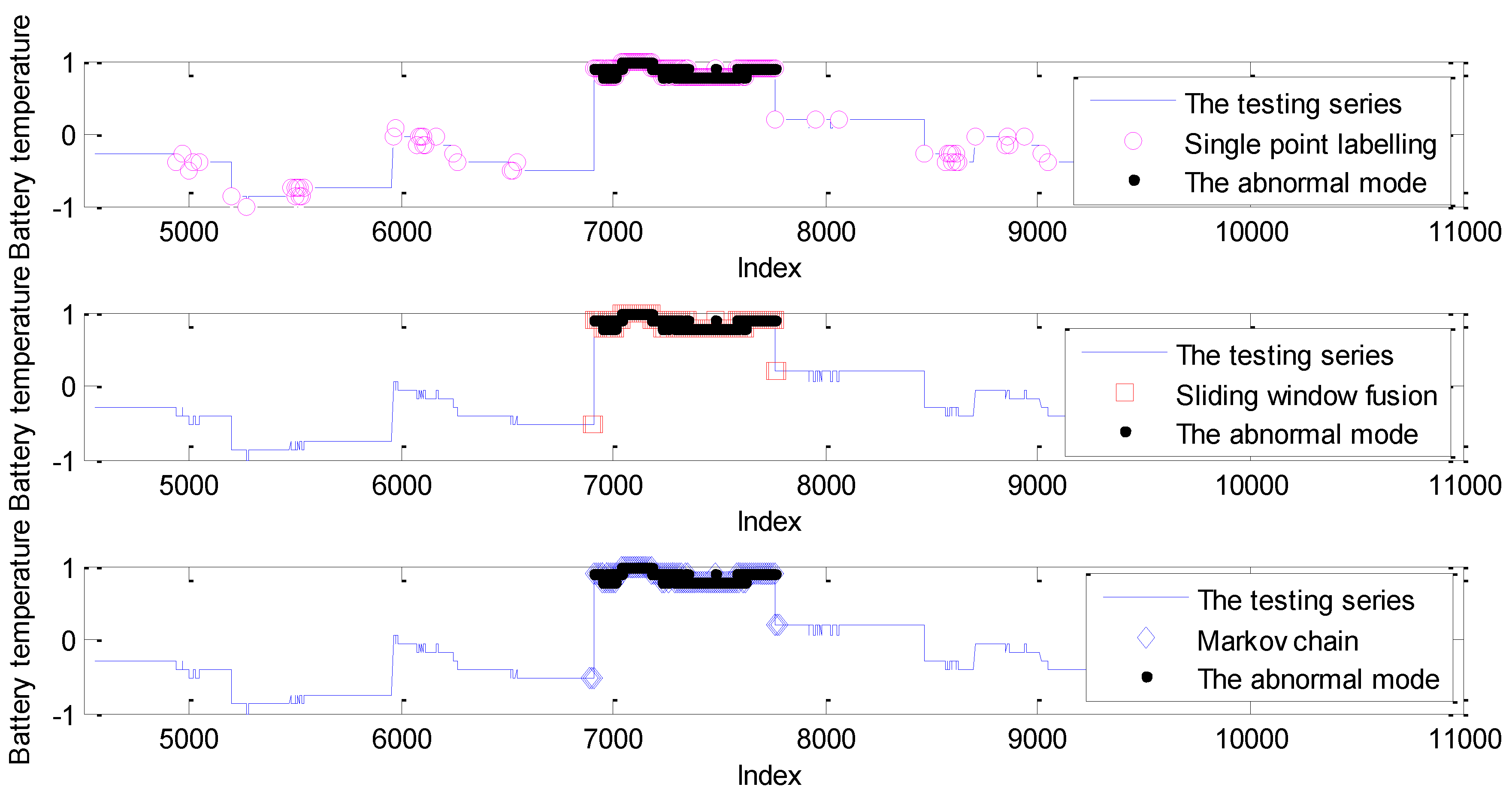
5.3. Case Study: Experiments on Telemetry Series with Anomalies
6. Conclusions
Author Contributions
Funding
Acknowledgments
Conflicts of Interest
References
- Fujimaki, R.; Yairi, T.; Machida, K. An approach to spacecraft anomaly detection problem using kernel feature space. In Proceedings of the Eleventh ACM SIGKDD International Conference on Knowledge Discovery in Data Mining, Chicago, IL, USA, 21–24 August 2005. [Google Scholar]
- Fuertes, S.; Picart, G.; Tourneret, J.Y.; Chaari, L.; Ferrari, A.; Richard, C. Improving Spacecraft Health Monitoring with Automatic Anomaly Detection Techniques. In Proceedings of the 14th International Conference on Space Operations, Daejeon, Korea, 16–20 May 2016. [Google Scholar]
- Kim, S.Y.; Castet, J.F.; Saleh, J.H. Spacecraft electrical power subsystem: Failure behavior, reliability, and multi-state failure analyses. Reliab. Eng. Syst. Saf. 2012, 98, 55–65. [Google Scholar] [CrossRef]
- Wu, J.; Yan, S.; Xie, L. Reliability analysis method of a solar array by using fault tree analysis and fuzzy reasoning Petri net. Acta Astronaut. 2011, 69, 960–968. [Google Scholar] [CrossRef]
- Song, Y.; Liu, D.; Hou, Y.; Yu, J.; Peng, Y. Satellite lithium-ion battery remaining useful life estimation with an iterative updated RVM fused with the KF algorithm. Chin. J. Aeronaut. 2018, 31, 31–40. [Google Scholar] [CrossRef]
- Yairi, T.; Oda, T.; Nakajima, Y.; Miura, N.; Takata, N. Evaluation Testing of Learning-based Telemetry Monitoring and Anomaly Detection System in SDS-4 Operation. In Proceedings of the International Symposium on Artificial Intelligence, Robotics and Automation in Space (i-SAIRAS), Montreal, QC, Canada, 17–19 June 2014. [Google Scholar]
- Rui, S. How the use of “Big Data” clusters improves off-line data analysis and operations. In Proceedings of the International Conference on Space Operations, Pasadena, CA, USA, 5–9 May 2014. [Google Scholar]
- Martínez-Heras, J.A.; Donati, A.; Sousa, B.; Fischer, J. DrMUST-a Data Mining Approach for Anomaly Investigation. In Proceedings of the SpaceOps 2012 Conference, Stockholm, Sweden, 11–15 June 2012. [Google Scholar]
- Bay, S.D.; Schwabacher, M. Mining distance-based outliers in near linear time with randomization and a simple pruning rule. In Proceedings of the ACM SIGKDD International Conference on Knowledge Discovery and Data Mining, Washington, DC, USA, 24–27 August 2003. [Google Scholar]
- Iverson, D. Data Mining Applications for Space Mission Operations System Health Monitoring. In Proceedings of the SpaceOps 2008 Conference, Heidelberg, Germany, 12–16 May 2008. [Google Scholar]
- Hundman, K.; Constantinou, V.; Laporte, C.; Colwell, I.; Soderstrom, T. Detecting Spacecraft Anomalies Using LSTMs and Nonparametric Dynamic Thresholding. In Proceedings of the 24th ACM SIGKDD International Conference on Knowledge Discovery and Data Mining, London, UK, 19–23 August 2018. [Google Scholar]
- Castet, J.F.; Saleh, J.H. Satellite Reliability: Statistical Data Analysis and Modeling. J. Spacecr. Rocket. 2009, 46, 1065–1076. [Google Scholar] [CrossRef]
- Zheng, L.; Jin, G.; Han, T.S. Fluctuation feature extraction of satellite telemetry data and on-orbit anomaly detection. In Proceedings of the Prognostics & System Health Management Conference, Chengdu, China, 19–21 October 2016. [Google Scholar]
- Zhang, Y.; Liu, L.; Peng, Y.; Liu, D. An Electro-Mechanical Actuator Motor Voltage Estimation Method with a Feature-Aided Kalman Filter. Sensors 2018, 18, 4190. [Google Scholar] [CrossRef] [PubMed]
- Liu, L.; Wang, S.; Liu, D.; Peng, Y. Quantitative Selection of Sensor Data Based on Improved Permutation Entropy for System Remaining Useful Life Prediction. Microelectron. Reliab. 2017, 75, 264–270. [Google Scholar] [CrossRef]
- Li, Q.; Zhou, X.; Lin, P.; Li, S. Anomaly detection and fault Diagnosis technology of spacecraft based on telemetry-mining. In Proceedings of the International Symposium on Systems & Control in Aeronautics & Astronautics, Harbin, China, 8–10 June 2010. [Google Scholar]
- Yairi, T.; Inui, M.; Kawahara, Y.; Takata, N. Spacecraft Telemetry Monitoring Method Based on Dimensionality Reduction and Clustering. J. Jpn. Soc. Aeronaut. Spaceences 2011, 59, 197–205. [Google Scholar] [CrossRef] [Green Version]
- Fujimaki, R.; Yairi, T.; Machida, K. Adaptive Limit-Checking for Spacecraft Using Sequential Prediction Based on Regression Techniques. J. Jpn. Soc. Aeronaut. Spaceences 2006, 54, 312–318. [Google Scholar] [CrossRef]
- Liu, D.; Pang, J.; Song, G.; Xie, W.; Peng, Y.; Peng, X. Fragment Anomaly Detection with Prediction and Statistical Analysis for Satellite Telemetry. IEEE Access 2017, 5, 19269–19281. [Google Scholar] [CrossRef]
- Xiong, L.; Ma, H.D.; Fang, H.Z. Anomaly detection of spacecraft based on least squares support vector machine. In Proceedings of the Prognostics & System Health Management Conference, Shenzhen, China, 24–25 May 2011. [Google Scholar]
- Fujimaki, R.; Yairi, T.; Machida, K. An Anomaly Detection Method for Spacecraft Using Relevance Vector Learning. In Proceedings of the Pacific-Asia Conference on Knowledge Discovery & Data Mining, Hanoi, Vietnam, 18–20 May 2005. [Google Scholar]
- Pang, J.; Liu, D.; Peng, Y.; Peng, X. Anomaly detection based on uncertainty fusion for univariate monitoring series. Measurement 2017, 95, 280–292. [Google Scholar] [CrossRef]
- Yairi, T.; Kawahara, Y.; Fujimaki, R.; Sato, Y.; Machida, K. Telemetry-mining: A Machine Learning Approach to Anomaly Detection and Fault Diagnosis for Space Systems. In Proceedings of the IEEE International Conference on Space Mission Challenges for Information Technology, Pasadena, CA, USA, 17–20 July 2006. [Google Scholar]
- Rasmussen, C.E. Gaussian Processes in Machine Learning. In Advanced Lectures on Machine Learning; Springer: Berlin/Heidelberg, Germany, 2004; pp. 63–71. [Google Scholar]
- Seeger, M. Gaussian Processes for Machine Learning. Int. J. Neural Syst. 2004, 14, 69–106. [Google Scholar] [CrossRef] [PubMed]
- Tipping, M.E. Sparse Bayesian Learning and Relevance Vector Machine. J. Mach. Learn. Res. 2001, 1, 211–244. [Google Scholar]
- Chandola, V.; Cheboli, D.; Kumar, V. Detecting Anomalies in a Time Series Database; CS Technical Report 09-004; Computer Science Department, University of Minnesota: Minneapolis, MN, USA, 2009. [Google Scholar]
- Zheludev, M.; Nagradov, E. Anomaly detection using Markov chain model. In Proceedings of the 2017 Computer Science and Information Technologies, Yerevan, Armenia, 25–29 September 2017. [Google Scholar]
- Sha, W.; Zhu, Y.; Huang, T. A Multi-order Markov Chain Based Scheme for Anomaly Detection. In Proceedings of the IEEE Computer Software & Applications Conference Workshops, Kyoto, Japan, 22–26 July 2013. [Google Scholar]
- Young, D.S.; Mills, T.M. Choosing a coverage probability for forecasting the incidence of cancer. Stat. Med. 2014, 33, 4104–4115. [Google Scholar] [CrossRef] [PubMed]
- Bontemps, L.; Cao, V.L.; Mcdermott, J.; Le-Khac, N. Collective Anomaly Detection Based on Long Short-Term Memory Recurrent Neural Networks. In Proceedings of the International Conference on Future Data and Security Engineering, Can Tho City, Vietnam, 23–25 November 2016. [Google Scholar]
- Keogh, E.; Lonardi, S.; Chiu, W. Finding surprising patterns in a time series database in linear time and space. In Proceedings of the Eighth ACM SIGKDD International Conference on Knowledge Discovery and Data Mining, Edmonton, AB, Canada, 23–26 July 2002. [Google Scholar]
- Chen, X.Y.; Zhan, Y.Y. Multi-scale anomaly detection algorithm based on infrequent pattern of time series. J. Comput. Appl. Math. 2008, 214, 227–237. [Google Scholar] [CrossRef] [Green Version]
- Guo, X.; Wang, D.; Chen, F. An anomaly detection based on data fusion algorithm in wireless sensor networks. Int. J. Distrib. Sens. Netw. 2015, 2015, 943532. [Google Scholar] [CrossRef]
- Chan, K.P.; Fu, W.C.; Yu, C. Data structures and algorithms haar wavelets for efficient similarity search of time series: With and without time warping. IEEE Trans. Knowl. Data Eng. 2003, 15, 686–705. [Google Scholar] [CrossRef]
- Allouche, O.; Tsoar, A.; Kadmon, R. Assessing the accuracy of species distribution models: Prevalence, kappa and the true skill statistic (TSS). J. Appl. Ecol. 2006, 43, 1223–1232. [Google Scholar] [CrossRef]


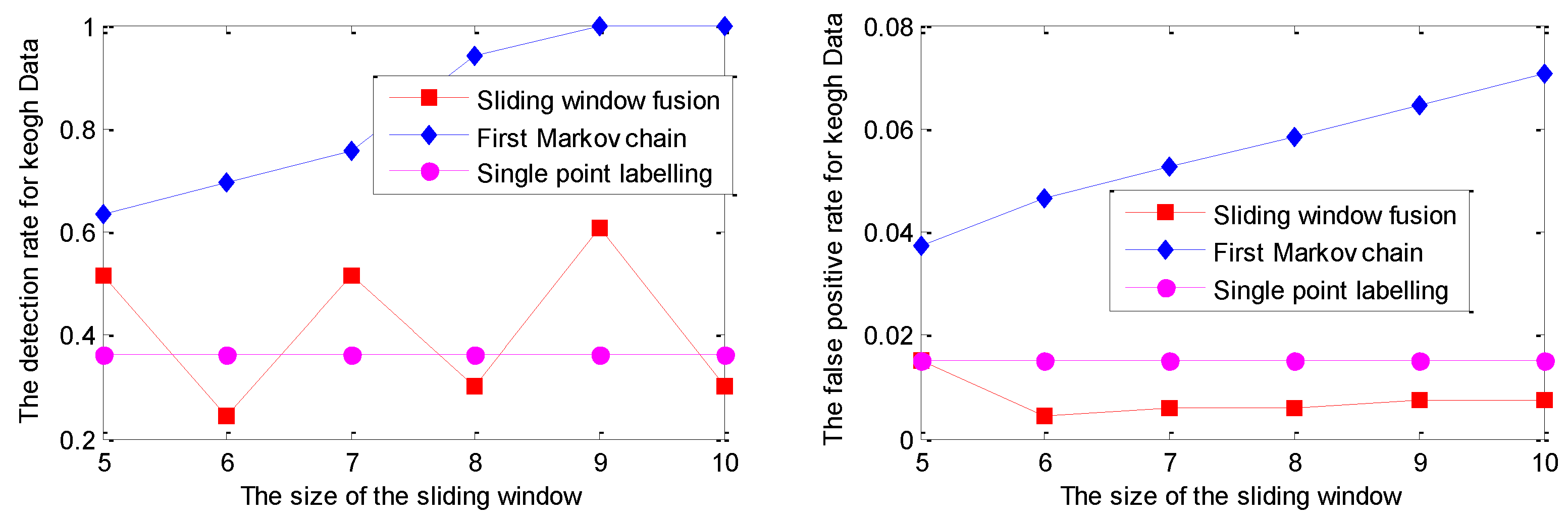
| Data/Model | Strategy | Indices | 5 | 6 | 7 | 8 | 9 | 10 |
|---|---|---|---|---|---|---|---|---|
| Keogh Data/GPR model | Single point | DR | 36.36% 1.50% | 36.36% 1.50% | 36.36% 1.50% | 36.36% 1.50% | 36.36% 1.50% | 36.36% 1.50% |
| FPR | ||||||||
| Sliding window | DR | 51.52% 1.50% | 24.24% 0.45% | 51.52% 0.60% | 30.30% 0.60% | 60.61% 0.75% | 30.30% 0.75% | |
| FPR | ||||||||
| Markov chain | DR | 84.85% | 90.91% | 96.97% | 100.00% | 100.00% | 100.00% | |
| FPR | 3.75% | 4.65% | 5.25% | 5.85% | 6.45% | 7.05% | ||
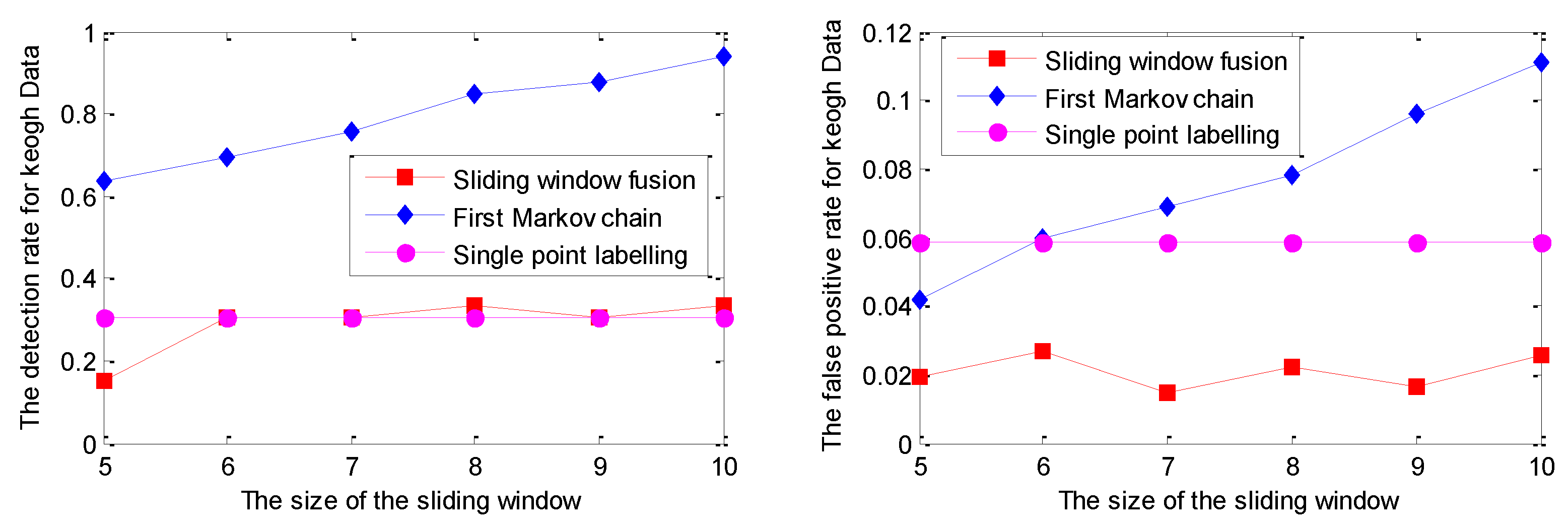
| Keogh Data/RVM model | Single point | DR | 30.30% 5.85% | 36.36% 1.50% | 36.36% 1.50% | 36.36% 1.50% | 36.36% 1.50% | 36.36% 1.50% |
| FPR | ||||||||
| Sliding window | DR | 15.15% 1.95% | 30.30% 2.70% | 30.30% 1.50% | 33.33% 2.25% | 30.30% 1.65% | 33.33% 2.55% | |
| FPR | ||||||||
| Markov chain | DR | 63.64% | 69.70% | 75.76% | 84.85% | 87.88% | 93.94% | |
| FPR | 4.20% | 6.00% | 6.90% | 7.80% | 9.60% | 11.09% | ||
| Ma Data/GPR model | Single point | DR | 48.48% 1.65% | 48.48% 1.65% | 48.48% 1.65% | 48.48% 1.65% | 48.48% 1.65% | 48.48% 1.65% |
| FPR | ||||||||
| Sliding window | DR | 63.64% 1.20% | 57.58% 0.00% | 72.73% 1.20% | 48.48% 0.00% | 51.52% 0.15% | 51.52% 0.15% | |
| FPR | ||||||||
| Markov chain | DR | 100.00% | 100.00% | 100.00% | 100.00% | 100.00% | 100.00% | |
| FPR | 4.05% | 4.95% | 5.25% | 5.55% | 5.85% | 6.15% | ||
| Ma Data/RVM model | Single point | DR | 66.70% 6.30% | 66.70% 6.30% | 66.70% 6.30% | 66.70% 6.30% | 66.70% 6.30% | 66.70% 6.30% |
| FPR | ||||||||
| Sliding window | DR | 81.82% 0.90% | 90.91% 2.25% | 90.91% 0.60% | 96.97% 2.25% | 96.97% 0.75% | 100.00% 1.05% | |
| FPR | ||||||||
| Markov chain | DR | 84.85% | 90.91% | 96.97% | 100.00% | 100.00% | 100.00% | |
| FPR | 3.00% | 4.20% | 4.95% | 5.55% | 4.95% | 5.55% |
| Data | Model | 5 | 6 | 7 | 8 | 9 | 10 |
|---|---|---|---|---|---|---|---|
| Keogh Data | GPR model | 81.10% | 86.26% | 91.72% | 94.15% | 93.55% | 92.95% |
| RVM model | 59.44% | 63.70% | 68.86% | 77.05% | 78.28% | 82.85% | |
| Ma Data | GPR model | 95.95% | 95.05% | 94.75% | 94.45% | 94.15% | 93.85% |
| RVM model | 81.85% | 86.71% | 92.02% | 94.45% | 95.05% | 94.45% |
| Data | Strategy | 5 | 6 | 7 | 8 | 9 | 10 |
|---|---|---|---|---|---|---|---|
| Solar voltage | Single point | 4.80% | 4.80% | 4.80% | 4.80% | 4.80% | 4.80% |
| Sliding window | 2.40% | 1.40% | 1.80% | 0.00% | 0.00% | 0.00% | |
| Markov chain | 1.00% | 2.60% | 4.80% | 3.60% | 2.00% | 3.40% | |
| Solar current | Single point | 2.80% | 2.80% | 2.80% | 2.80% | 2.80% | 2.80% |
| Sliding window | 1.00% | 0.00% | 0.00% | 0.00% | 0.00% | 0.00% | |
| Markov chain | 2.20% | 4.20% | 5.40% | 5.60% | 2.60% | 3.00% | |
| Battery voltage | Single point | 3.40% | 3.40% | 3.40% | 3.40% | 3.40% | 3.40% |
| Sliding window | 3.20% | 1.80% | 2.22% | 2.22% | 2.60% | 0.00% | |
| Markov chain | 0.00% | 0.00% | 1.40% | 1.80% | 2.20% | 2.60% | |
| Solar temperature | Single point | 3.80% | 3.80% | 3.80% | 3.80% | 3.80% | 3.80% |
| Sliding window | 6.00% | 3.40% | 4.20% | 2.20% | 2.60% | 0.00% | |
| Markov chain | 4.00% | 5.00% | 6.20% | 7.40% | 5.40% | 0.00% |
| Telemetry Series | 4 | 5 | 6 | 7 | 8 |
|---|---|---|---|---|---|
| Solar voltage | 6.60% | 3.00% | 0.00% | 0.00% | 0.00% |
| Data | Strategy | FPR | DR |
|---|---|---|---|
| Battery temperature | Single point labelling | 1.45% | 100.00% |
| Sliding window Fusion | 0.42% | 100.00% | |
| Markov chain | 0.75% | 100.00% |
© 2019 by the authors. Licensee MDPI, Basel, Switzerland. This article is an open access article distributed under the terms and conditions of the Creative Commons Attribution (CC BY) license (http://creativecommons.org/licenses/by/4.0/).
Share and Cite
Pang, J.; Liu, D.; Peng, Y.; Peng, X. Collective Anomalies Detection for Sensing Series of Spacecraft Telemetry with the Fusion of Probability Prediction and Markov Chain Model. Sensors 2019, 19, 722. https://0-doi-org.brum.beds.ac.uk/10.3390/s19030722
Pang J, Liu D, Peng Y, Peng X. Collective Anomalies Detection for Sensing Series of Spacecraft Telemetry with the Fusion of Probability Prediction and Markov Chain Model. Sensors. 2019; 19(3):722. https://0-doi-org.brum.beds.ac.uk/10.3390/s19030722
Chicago/Turabian StylePang, Jingyue, Datong Liu, Yu Peng, and Xiyuan Peng. 2019. "Collective Anomalies Detection for Sensing Series of Spacecraft Telemetry with the Fusion of Probability Prediction and Markov Chain Model" Sensors 19, no. 3: 722. https://0-doi-org.brum.beds.ac.uk/10.3390/s19030722