Performance Evaluation and Interference Characterization of Wireless Sensor Networks for Complex High-Node Density Scenarios

 ,
,  ,
,  ,
,  and
and 
Abstract
:1. Introduction
2. Proposed Simulation Technique
2.1. The RL Technique
- -
- Creation of the 3D environment.
- -
- Simulation procedure.
- -
- Results analysis.
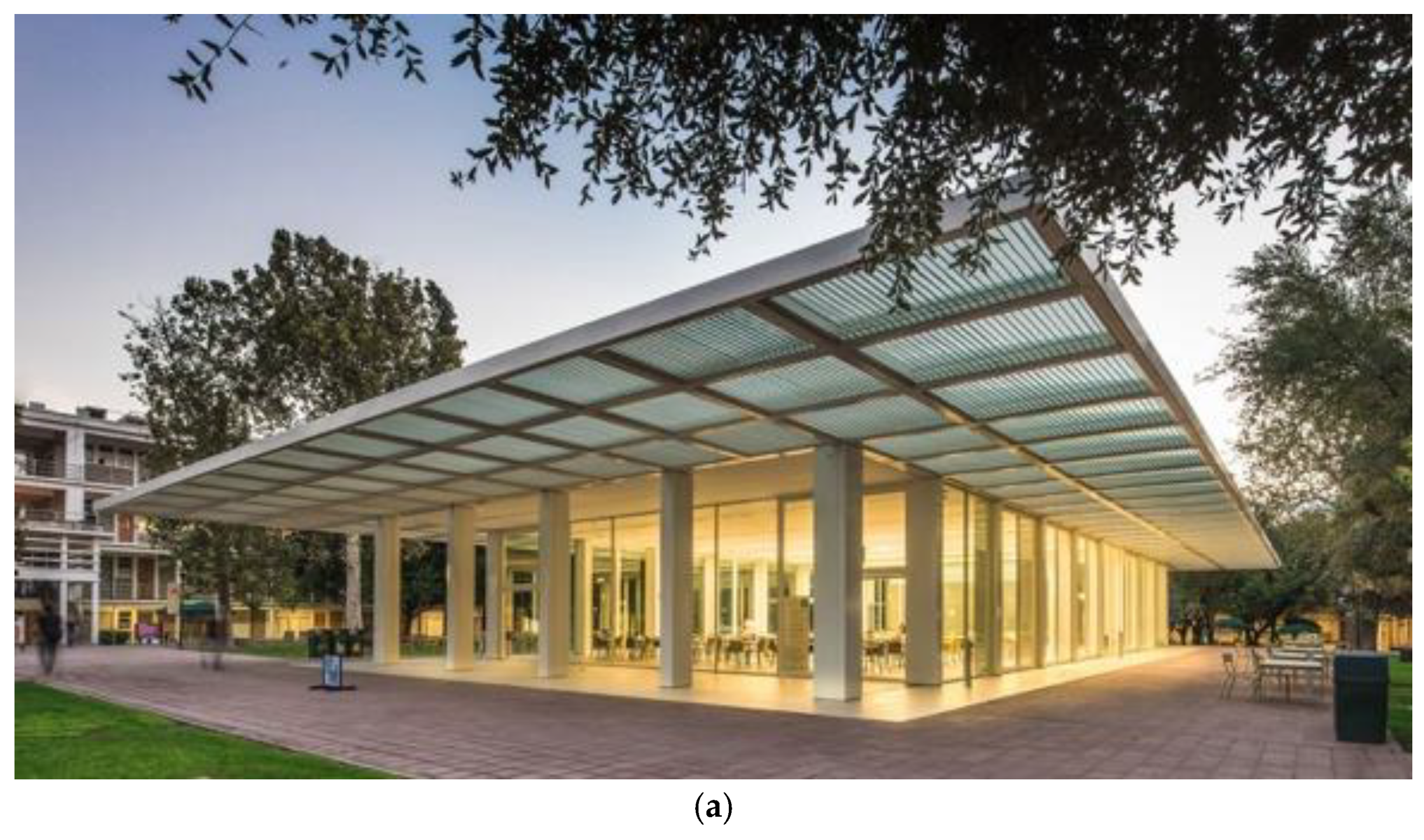
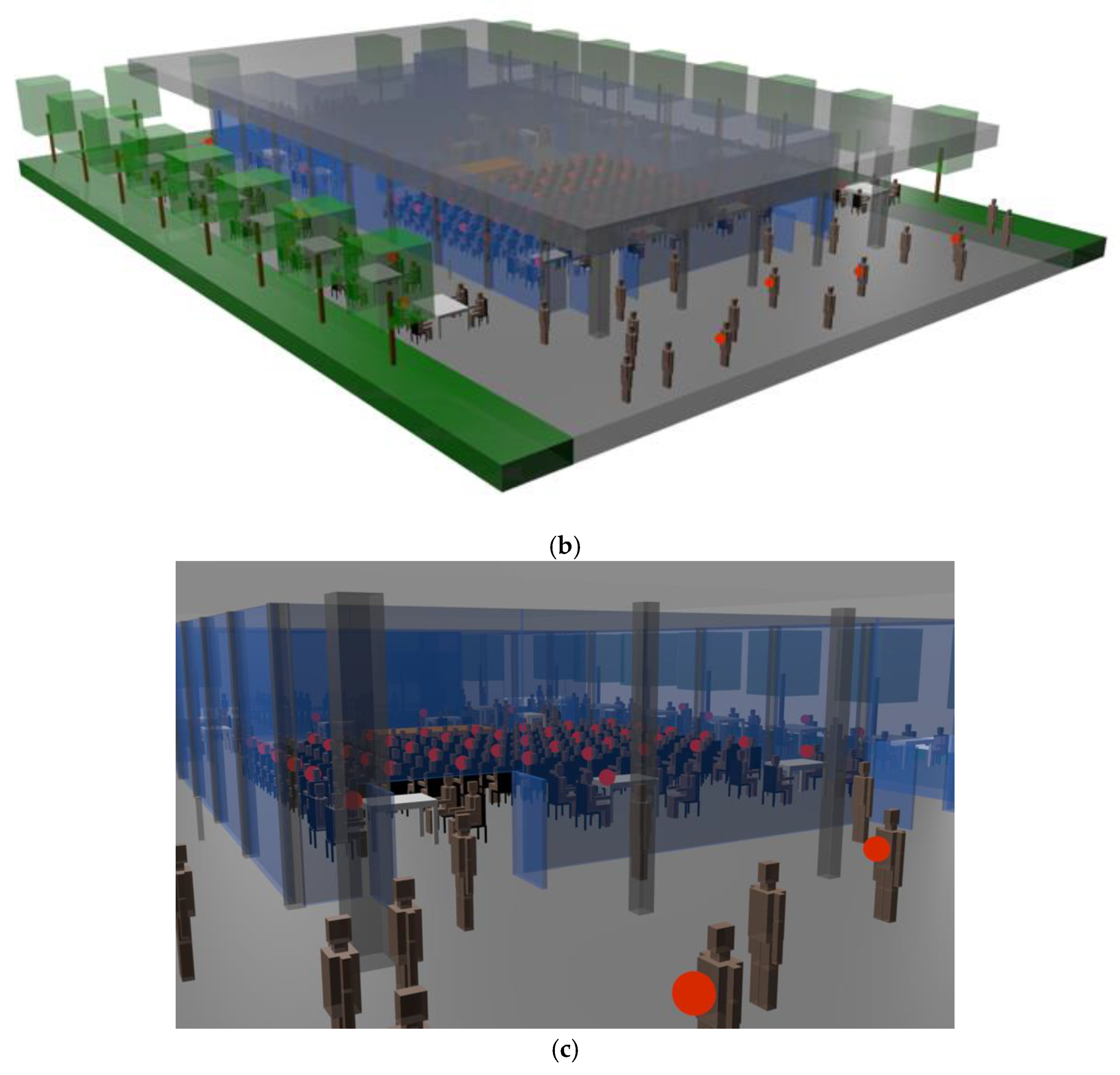
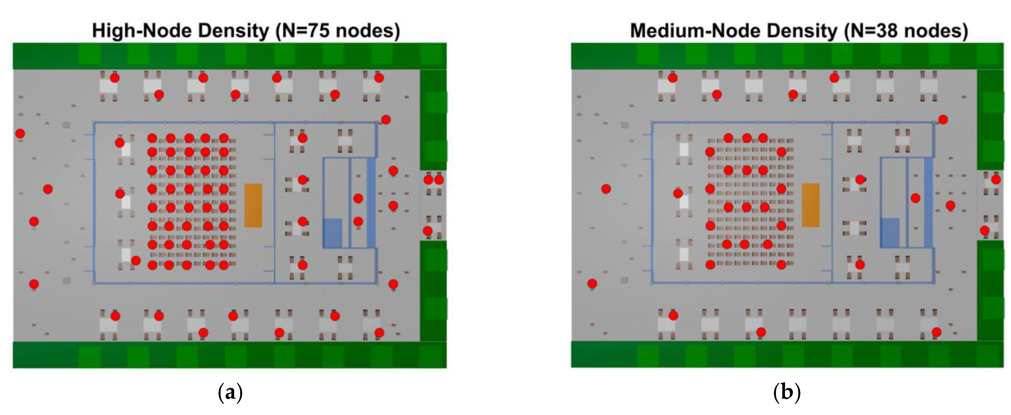
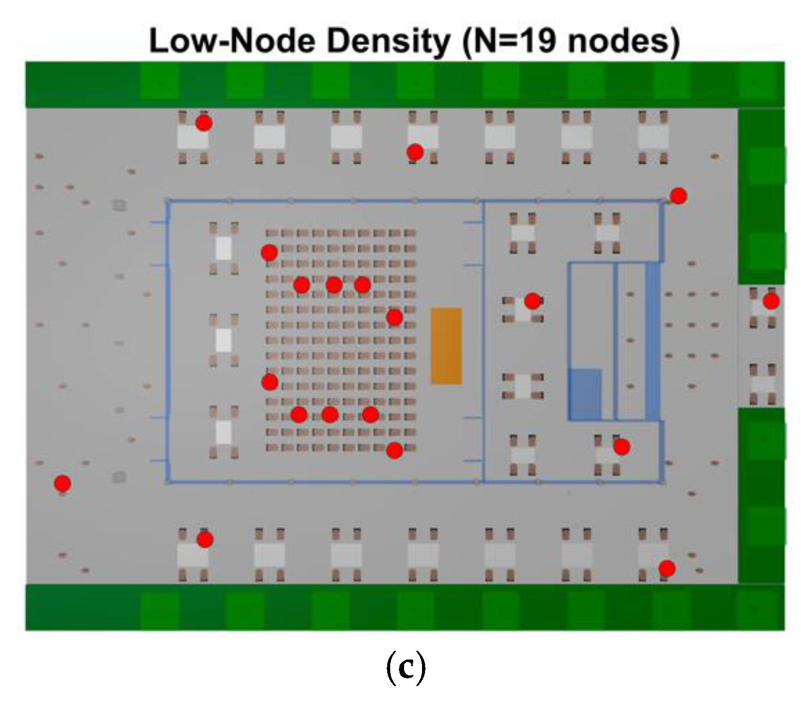
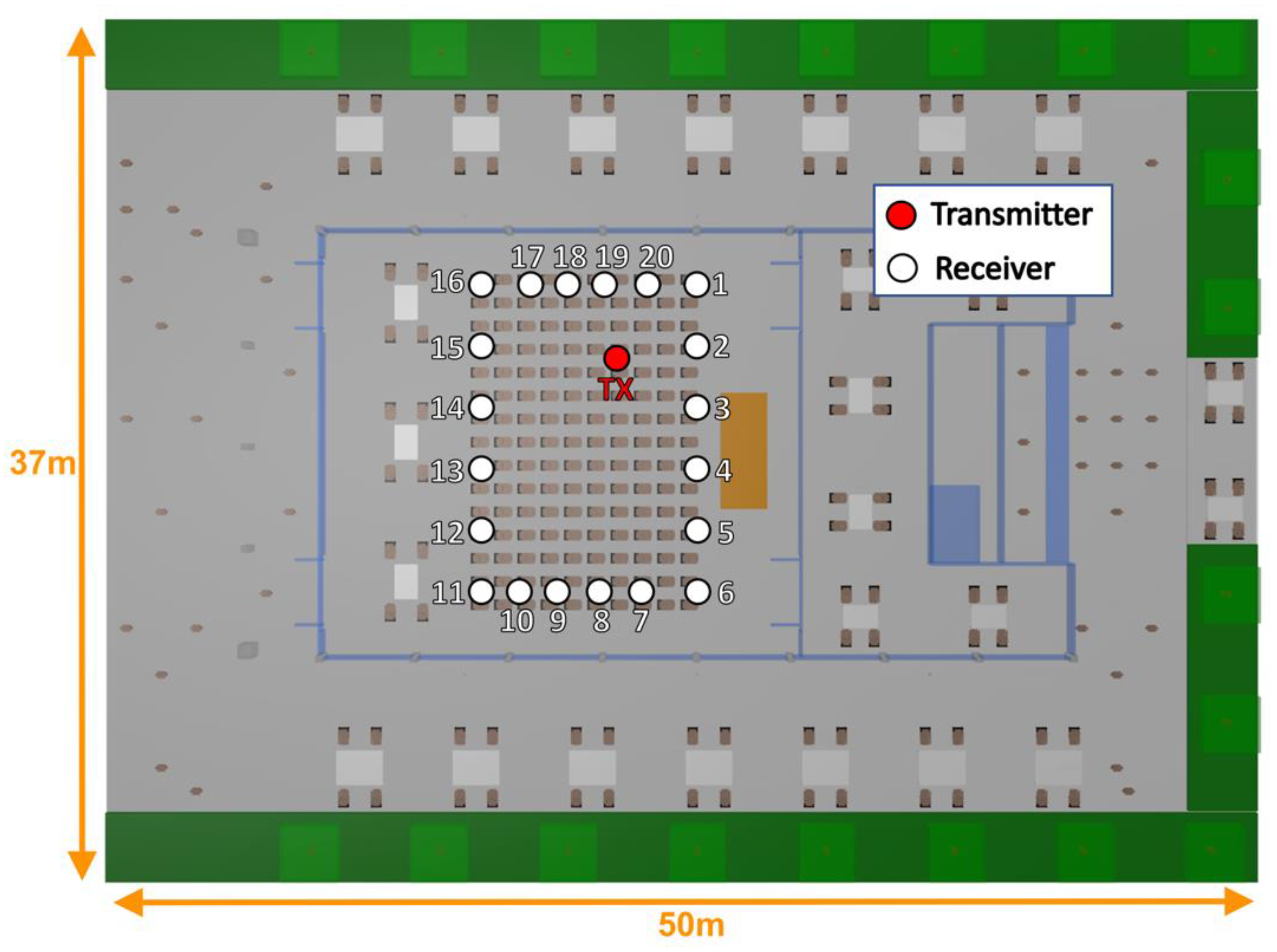
2.2. Scenario Description
3. Simulation Results
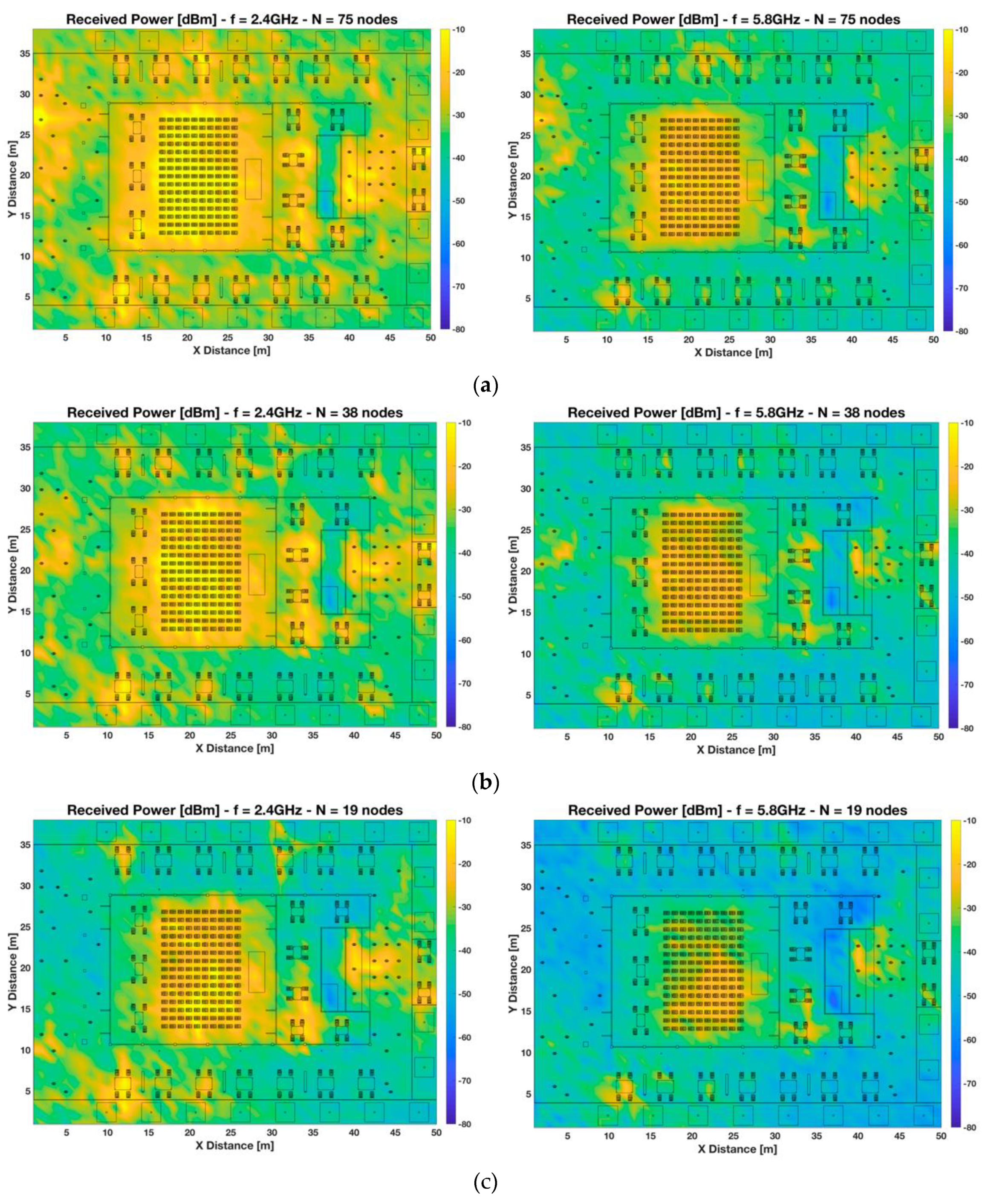
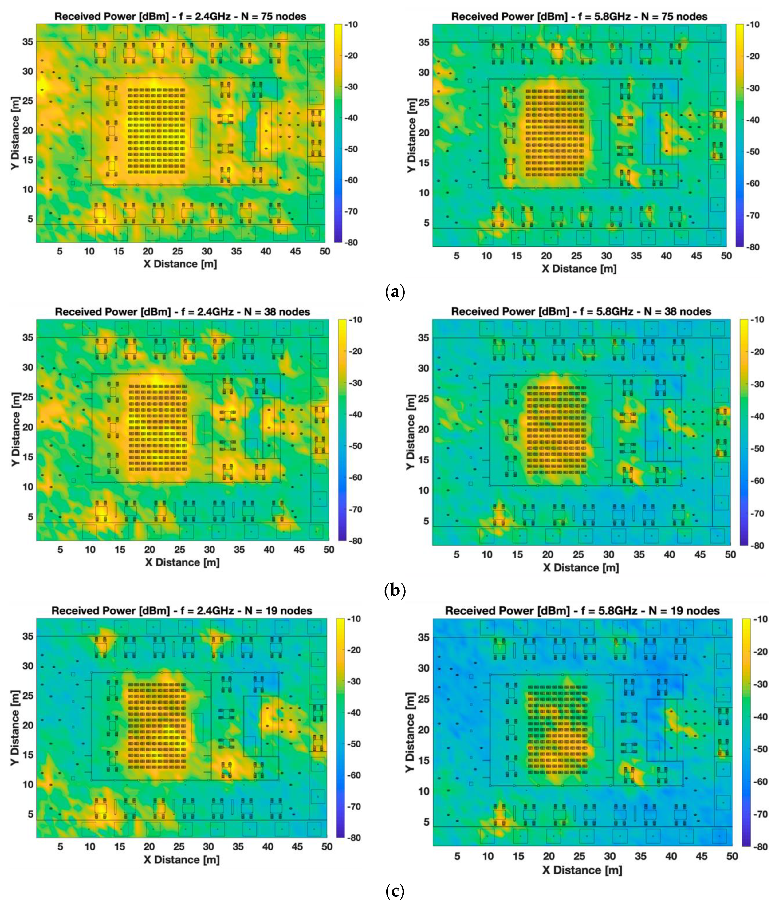
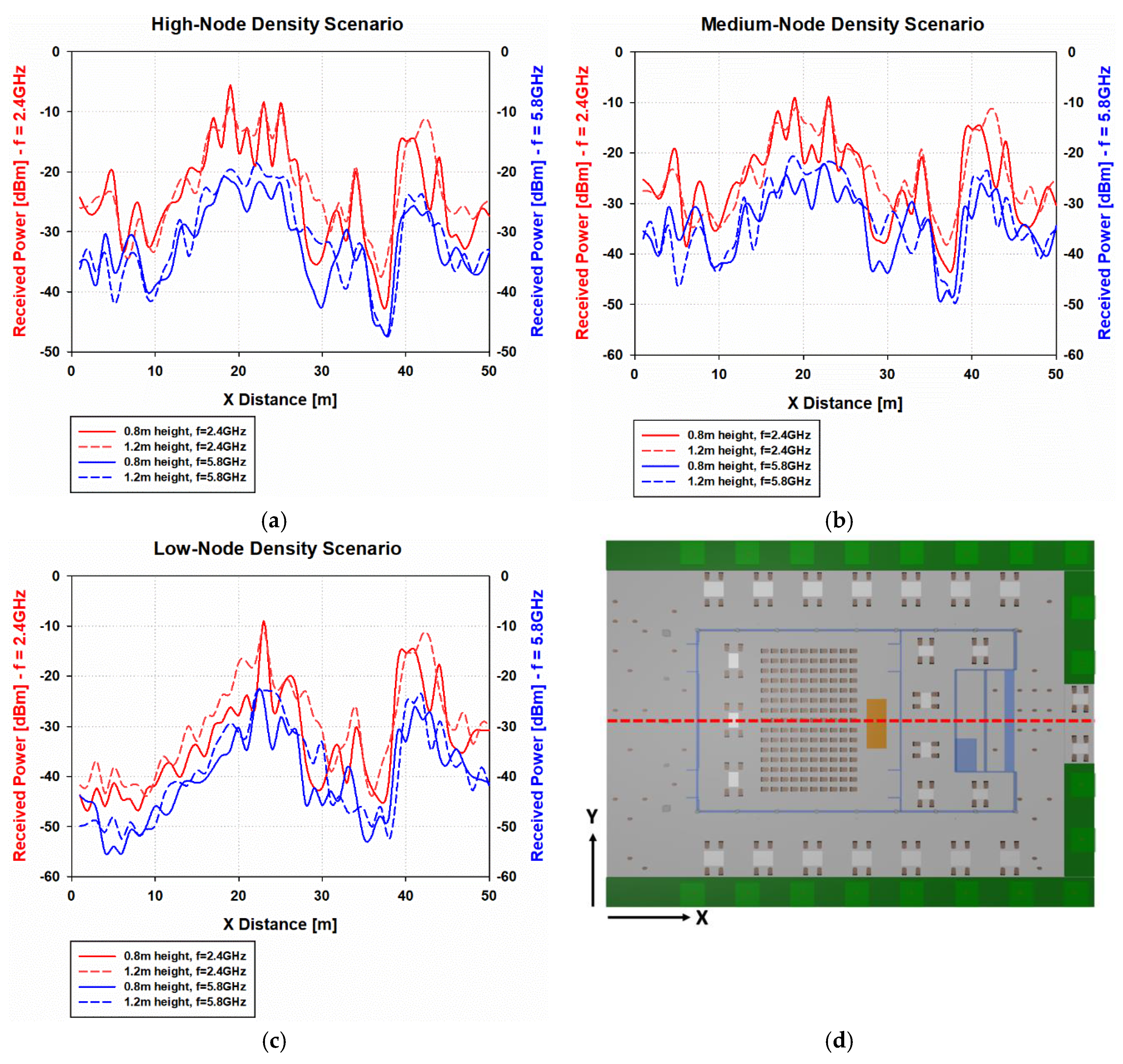
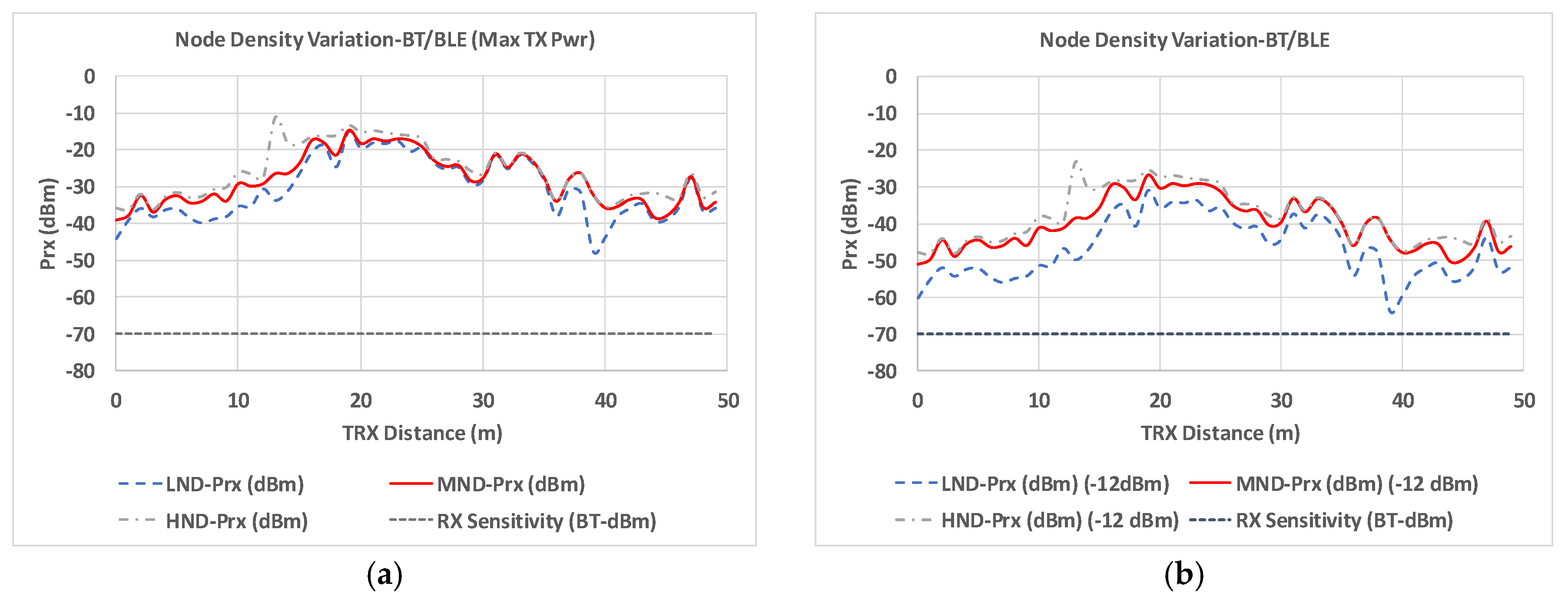
3.1. Received Signal Strength
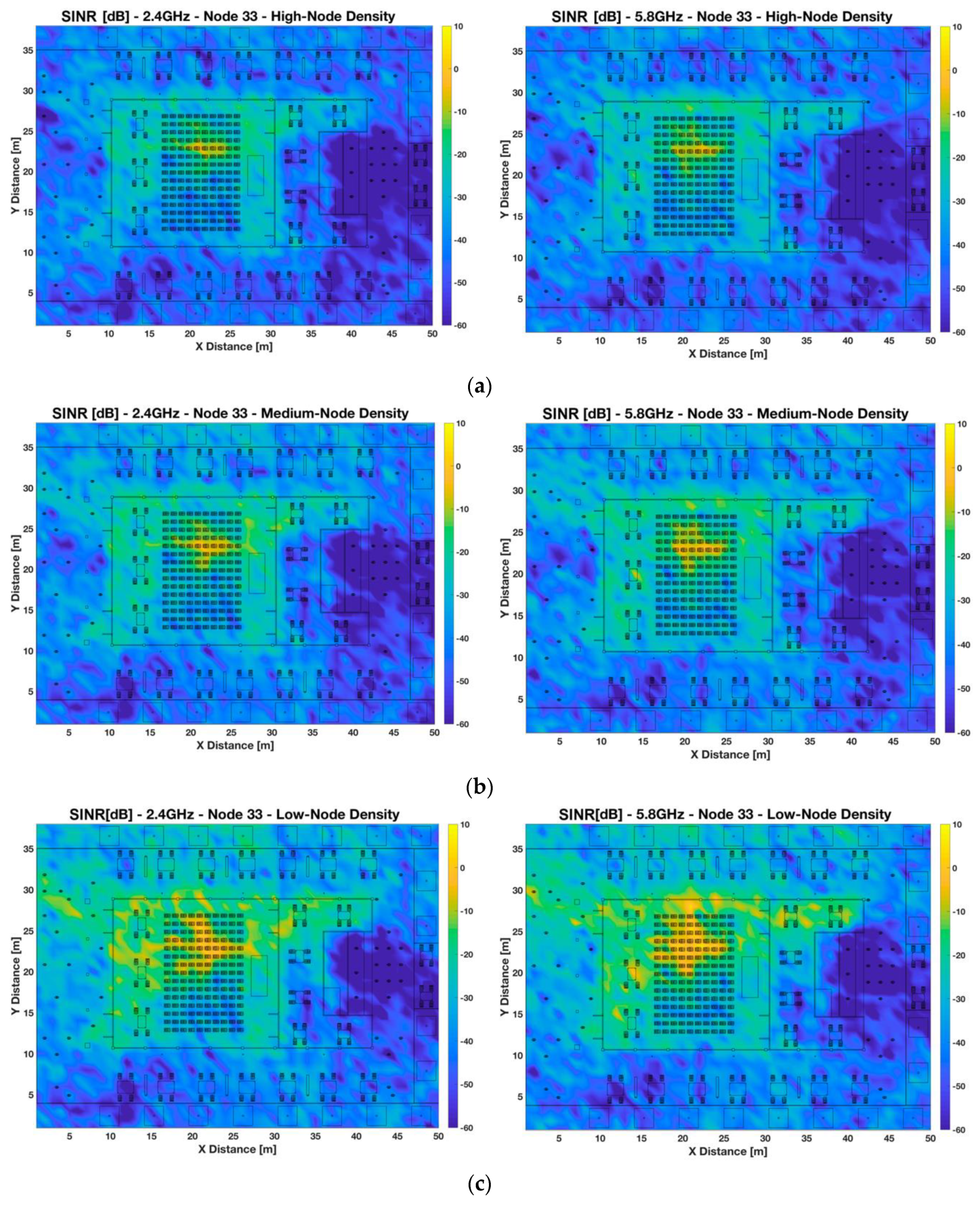
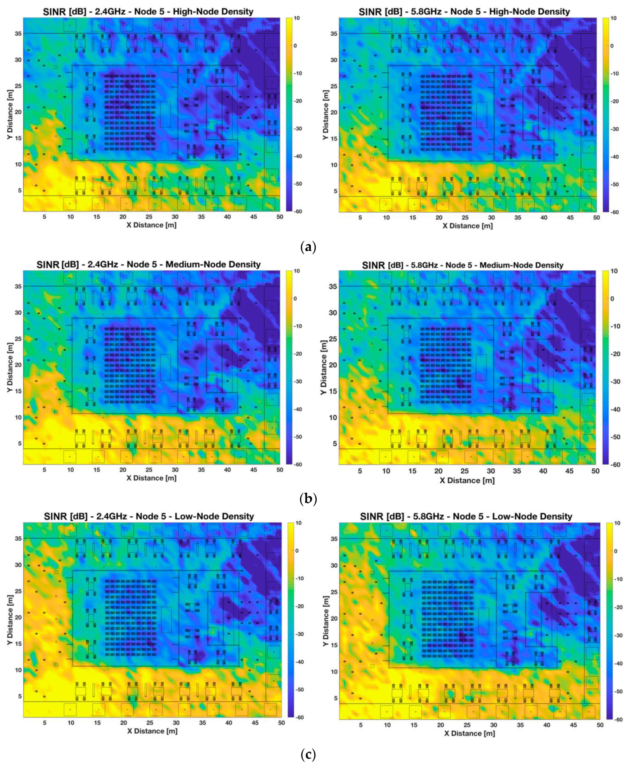
3.2. Signal to Interference Noise Ratio
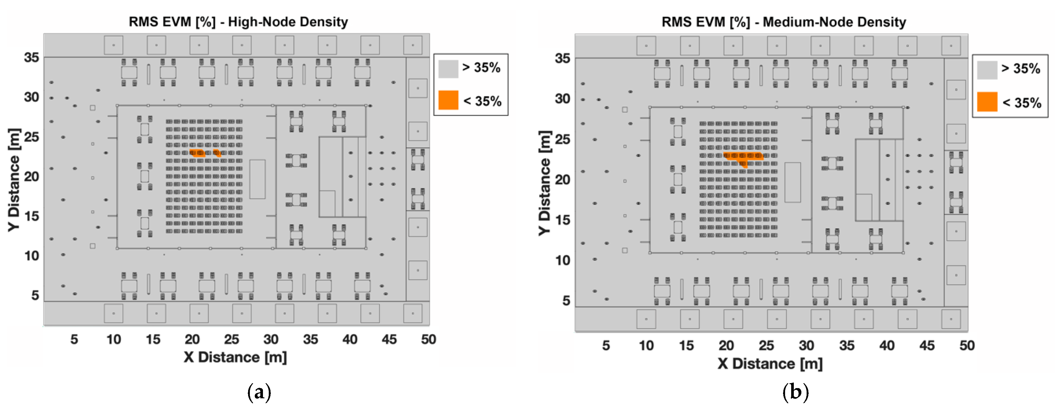
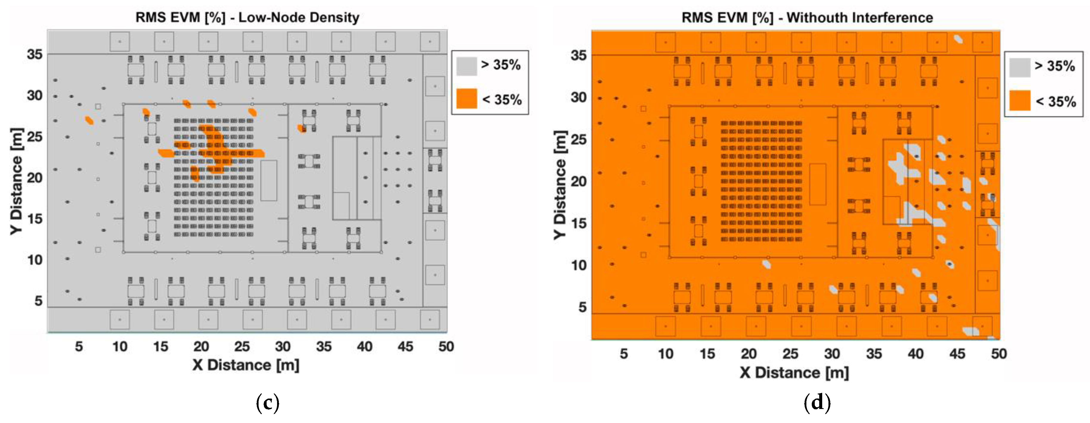
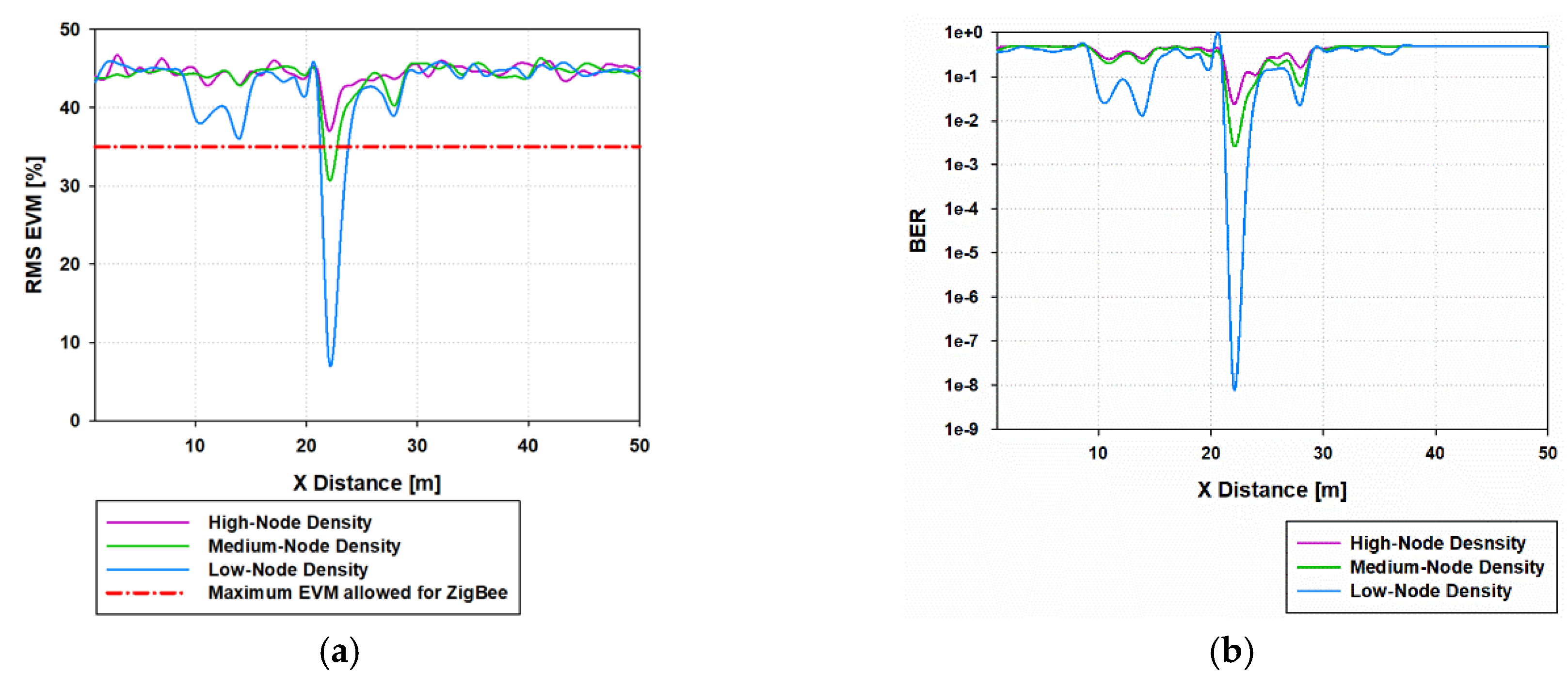
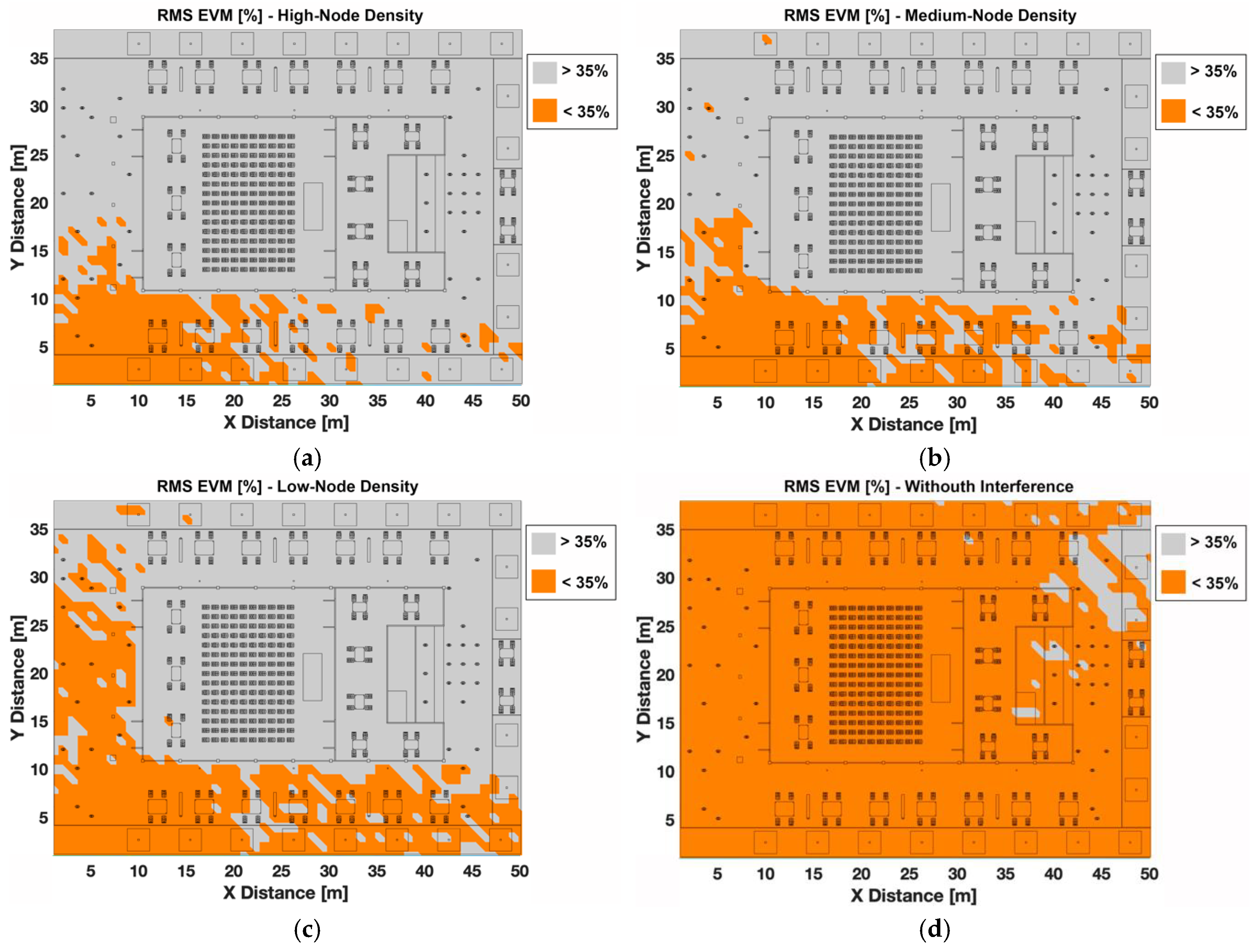
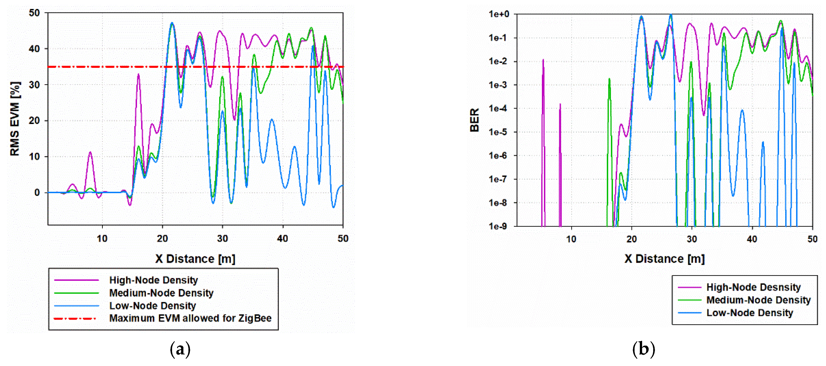
3.3. Performance Analysis
4. Measurements Campaign
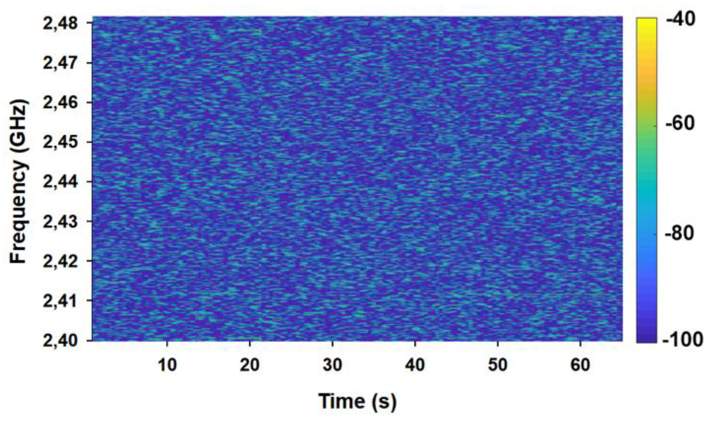
4.1. Experimental Setup
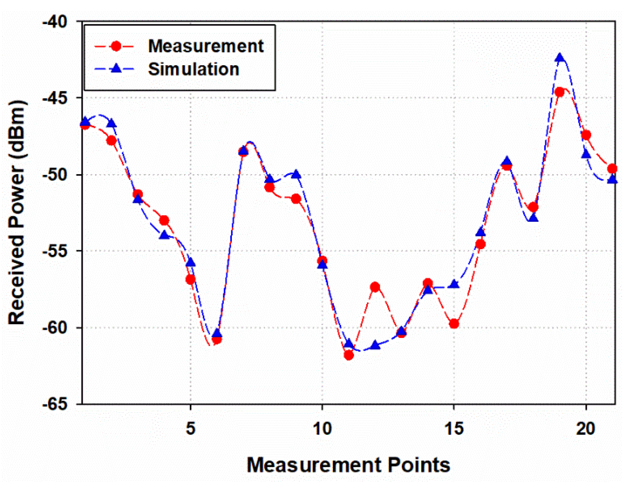
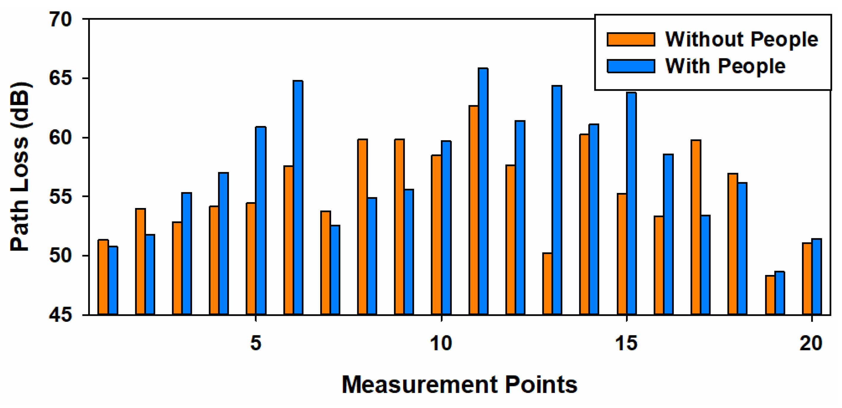
4.2. Measurements Results
5. Conclusions and Future Work
Author Contributions
Funding
Acknowledgments
Conflicts of Interest
References
- Stankovic, J.A. Research Directions for the Internet of Things. IEEE Internet Things J. 2014, 1, 3–9. [Google Scholar] [CrossRef]
- Bradshaw, V. The Building Environment: Active and Passive Control Systems; Wiley: Hoboken, NJ, USA, 2006. [Google Scholar]
- Zeiler, W.; Houten, R.; Boxem, G.; Vissers, D.; Maaijen, R. Indoor air quality and thermal comfort strategies: The human-in-the-loop approach. In Proceedings of the 11th International Conference for Enhanced Building (ICEBO 2011), New York, NY, USA, 18–20 October 2011. [Google Scholar]
- Burnham, G.; Seo, J.; Bekey, G.A. Identification of human driver models in car following. IEEE Trans. Autom. Control 1974, 19, 911–915. [Google Scholar] [CrossRef]
- Control4 Home Automation and Control [Online]. Available online: http://www.control4.com (accessed on 23 January 2019).
- M1 Security and Automation Controls [Online]. Available online: http://www.elkproducts.com/m1 controls.html (accessed on 23 January 2019).
- Dickerson, R.; Gorlin, E.; Stankovic, J. Empath: A continuous remote emotional health monitoring system for depressive illness. In Proceedings of the 2nd Conference on Wireless Health, San Diego, CA, USA, 10–13 October 2011. [Google Scholar]
- World’s Population Increasingly Urban with More Than Half Living in Urban Areas; United Nat: New York, NY, USA, 2014; Available online: http://www.un.org/en/development/desa/news/population/world-urbanization-prospects-2014.html (accessed on 23 January 2019).
- Evans, D. The Internet of Things: How the Next Evolution of the Internet Is Changing Everything. 2011. Available online: http://www.cisco.com/c/dam/en_us/about/ac79/docs/innov/IoT_IBSG_0411FINAL.pdf (accessed on 23 January 2019).
- Gharaibeh, A. Smart Cities: A Survey on Data Management, Security, and Enabling Technologies. IEEE Commun. Surv. Tutor. 2017, 19, 2456–2501. [Google Scholar] [CrossRef]
- Al-Dulaimi, A.; Al-Rubaye, S.; Cosmas, J.; Anpalagan, A. Planning of Ultra-Dense Wireless Networks. IEEE Netw. 2017, 31, 90–96. [Google Scholar] [CrossRef]
- Lee, S.; Kim, S.; Park, Y.; Choi, S.; Hong, D. Effect of Unpredictable Interference on MU-MIMO Systems in HetNet. IEEE Access 2018, 6, 28870–28876. [Google Scholar] [CrossRef]
- Park, Y.; Hong, D. Theoretical Analysis of Interference Effect from Idle Cells in Ultra-Dense Small Cell Networks. IEEE Access 2018, 6, 26881–26894. [Google Scholar] [CrossRef]
- Liu, Z.; Liu, J.; Zeng, Y.; Ma, J. Covert Wireless Communications in IoT Systems: Hiding Information in Interference. IEEE Wirel. Commun. 2018, 25, 46–52. [Google Scholar] [CrossRef]
- Yao, K.; Wu, Q.; Xu, Y.; Jing, J. Distributed ABS-Slot Access in Dense Heterogeneous Networks: A Potential Game Approach with Generalized Interference Model. IEEE Access 2017, 5, 94–104. [Google Scholar] [CrossRef]
- Fu, S.; Su, Z.; Jia, Y.; Zhou, H.; Jin, Y.; Ren, J.; Wu, B.; Huq, S.K.M. Interference Cooperation via Distributed Game in 5G Networks. IEEE Internet Things J. 2019, 6, 311–320. [Google Scholar] [CrossRef]
- Zhang, L.; Ijaz, A.; Xiao, P.; Tafazolli, R. Channel Equalization and Interference Analysis for Uplink Narrowband Internet of Things (NB-IoT). IEEE Commun. Lett. 2017, 21, 2206–2210. [Google Scholar] [CrossRef]
- Croce, D.; Gucciardo, M.; Mangione, S.; Santaromita, G.; Tinnirello, I. Impact of LoRa Imperfect Orthogonality: Analysis of Link-Level Performance. IEEE Commun. Lett. 2018, 22, 796–799. [Google Scholar] [CrossRef] [Green Version]
- Kishk, M.A.; Dhillon, H.S. Joint Uplink and Downlink Coverage Analysis of Cellular-based RF-powered IoT Network. IEEE Trans. Green Commun. Netw. 2018, 2, 446–459. [Google Scholar] [CrossRef]
- Malik, H.; Pervaiz, H.; Alam, M.M.; Le Moullec, Y.; Kuusik, A.; Imran, A.M. Radio Resource Management Schemein NB-IoT Systems. IEEE Access 2018, 6, 15051–15064. [Google Scholar] [CrossRef]
- Baidya, S.; Levorato, M. Content-Aware Cognitive Interference Control for Urban IoT Systems. IEEE Trans. Cogn. Commun. Netw. 2018, 4, 500–512. [Google Scholar] [CrossRef]
- Lee, H.; Park, Y.; Hong, D. Resource Split Full Duplex to Mitigate Inter-Cell Interference in Ultra-Dense Small Cell Networks. IEEE Access 2018, 6, 37653–37664. [Google Scholar] [CrossRef]
- Lynggaard, P. Using Machine Learning for Adaptive Interference Suppression in Wireless Sensor Networks. IEEE Sens. J. 2018, 18, 8820–8826. [Google Scholar] [CrossRef]
- Gu, Y.; Cui, Q.; Chen, Y.; Ni, W.; Tao, X.; Zhang, P. Effective Capacity Analysis in Ultra-Dense Wireless Networks with Random Interference. IEEE Access 2018, 6, 19499–19508. [Google Scholar] [CrossRef]
- Jiang, N.; Deng, Y.; Kang, X.; Nallanathan, A. Random Access Analysis for Massive IoT Networks Under a New Spatio-Temporal Model: A Stochastic Geometry Approach. IEEE Trans. Commun. 2018, 66, 5788–5803. [Google Scholar] [CrossRef] [Green Version]
- Grimaldi, S.; Mahmood, A.; Gidlund, M. Real-Time Interference Identification via Supervised Learning: Embedding Coexistence Awareness in IoT Devices. IEEE Access 2019, 7, 835–850. [Google Scholar] [CrossRef]
- Sha, M.; Hackmann, C.G. Real-World Empirical Studies on Multi-Channel Reliability and Spectrum Usage for Home-Area Sensor Networks. IEEE Trans Netw. Serv. Manag. 2013, 10, 56–69. [Google Scholar] [CrossRef]
- Shen, Y.; Wymeersch, H.; Moe, Z.W. Fundamental Limits of Wideband Localization—Part II: Cooperative Networks. IEEE Trans Inf. 2010, 56, 4981–5000. [Google Scholar] [CrossRef]
- Yuan, W.; Wu, N.; Etzlinger, B.; Li, Y.; Yan, C.; Hanzo, L. Expectation Maximization-Based Passive Localization Relying on Asynchronous Receivers: Centralized versus Distributed Implementations. IEEE Trans. Commmun. 2019, 67, 668–681. [Google Scholar] [CrossRef]
- Xiong, Y.; Wu, M.N.; Shen, Y.; Win, M.Z. Cooperative Network Synchronization: Asymptotic Analysis. IEEE Trans. Sign. Proc. 2018, 66, 757–772. [Google Scholar] [CrossRef]
- Mostafaei, H.; Montieri, A.; Persico, V.; Pescape, A. A sleep shceduling approach based on learning automata for WSN partial coverage. J. Netw. Comp. Appl. 2017, 80, 67–78. [Google Scholar] [CrossRef]
- Azpilicueta, L.; Rawat, M.; Rawat, K.; Ghannouchi, F.; Falcone, F. Convergence analysis in deterministic 3D ray launching radio channel estimation in complex environments. Appl. Comput. Electromagn. Soc. J. 2014, 29, 256–271. [Google Scholar]
- Azpilicueta, L.; Vargas-Rosales, C.; Falcone, F. Deterministic Propagation Prediction in Transportation Systems. IEEE Veh. Technol. Mag. 2016, 11, 29–37. [Google Scholar] [CrossRef]
- Azpilicueta, L.; López-Iturri, P.; Aguirre, E.; Falcone, F. An accurate UTD Extension to a Ray Launching Algorithm for the Analysis of Complex Indoor Radio Environments. J. Electromagn. Waves Appl. 2016, 30, 43–60. [Google Scholar] [CrossRef]
- Hall, P.S.; Hao, Y. Antennas and Propagation for Body-Centric Wireless Communications, 2nd ed.; Artech House: Norwood, MA, USA, 2012. [Google Scholar]
- Aguirre, E.; Arpón, J.; Azpilicueta, L.; De Miguel, S.; Ramos, V.; Falcone, F. Evaluation of Electromagnetic Dosimetry of Wireless Systems in Complex Indoor Scenarios with human body interaction. Pier B 2012, 43, 189–209. [Google Scholar] [CrossRef]
- Lopez-Iturri, P.; Aguirre, E.; Azpilicueta, L.; Astrain, J.J.; Villadangos, J.; Falcone, F. Challenges in Wireless System Integration as Enablers for Indoor Context Aware Environments. Sensors 2017, 17, 1616. [Google Scholar] [CrossRef]
- IEEE 802.15.4: Wireless Medium Access Control (MAC) and Physical Layer (PHY) Specifications for Low-Rate Wireless Personal Area Networks (WPANs); IEEE: Piscataway, NY, USA, 2006.
- Koutitas, G. Multiple Human Effects in Body Area Networks. IEEE Antennas Wirel. Propag. Lett. 2010, 9, 938–941. [Google Scholar] [CrossRef]


| Parameters | Values |
|---|---|
| Wearable TX Power | 4 dBm |
| Frequency | 2.4GHz/5.8 GHz |
| Bit Rate | 250 kbps/1 Mbps/3 Mbps |
| Antenna Radiation Pattern (RX, TX)/Gain | Omnidirectional/0 dB |
| 3D Ray Launching: Angular Resolution/Reflections | 1 degree/6 |
| Scenario size/Unitary volume analysis | (50 × 37 × 8) m/1 m3 (1 × 1 × 1) m |
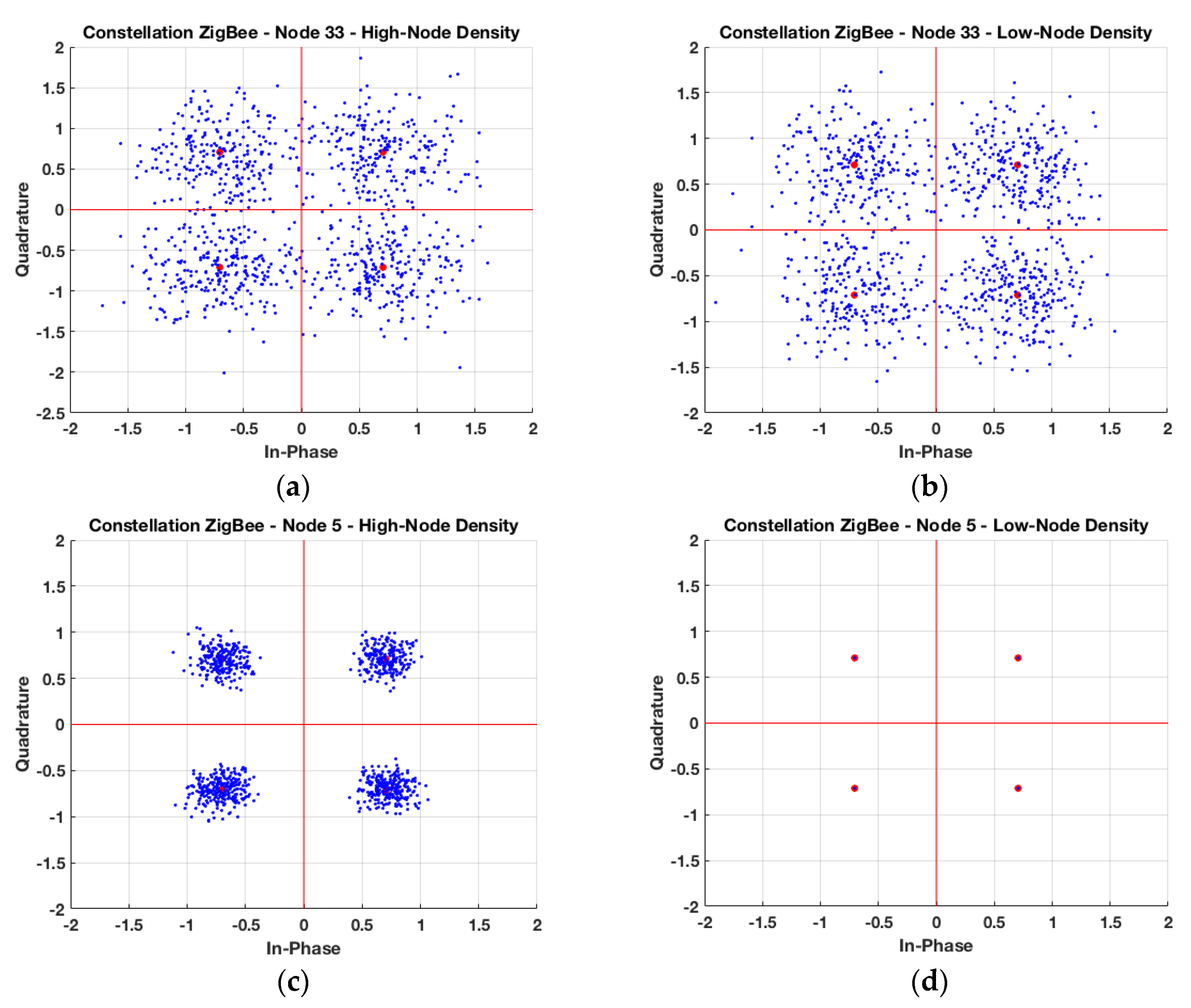
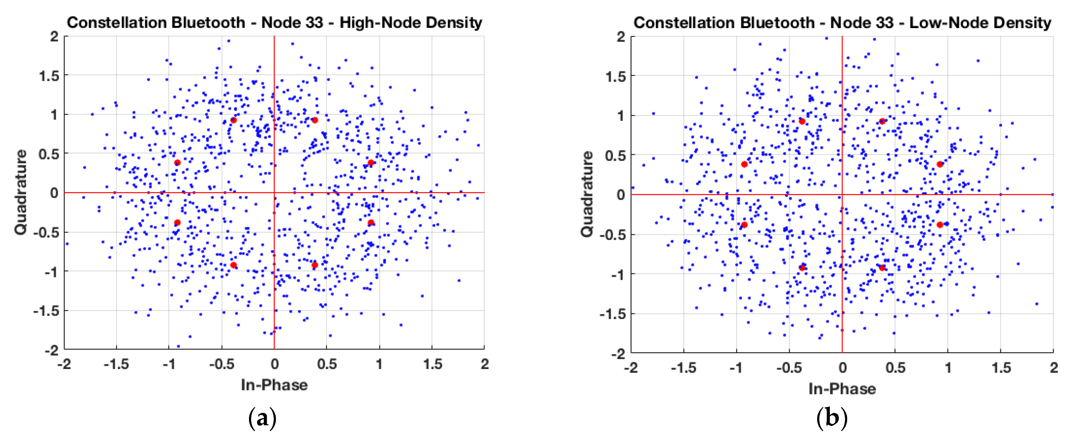
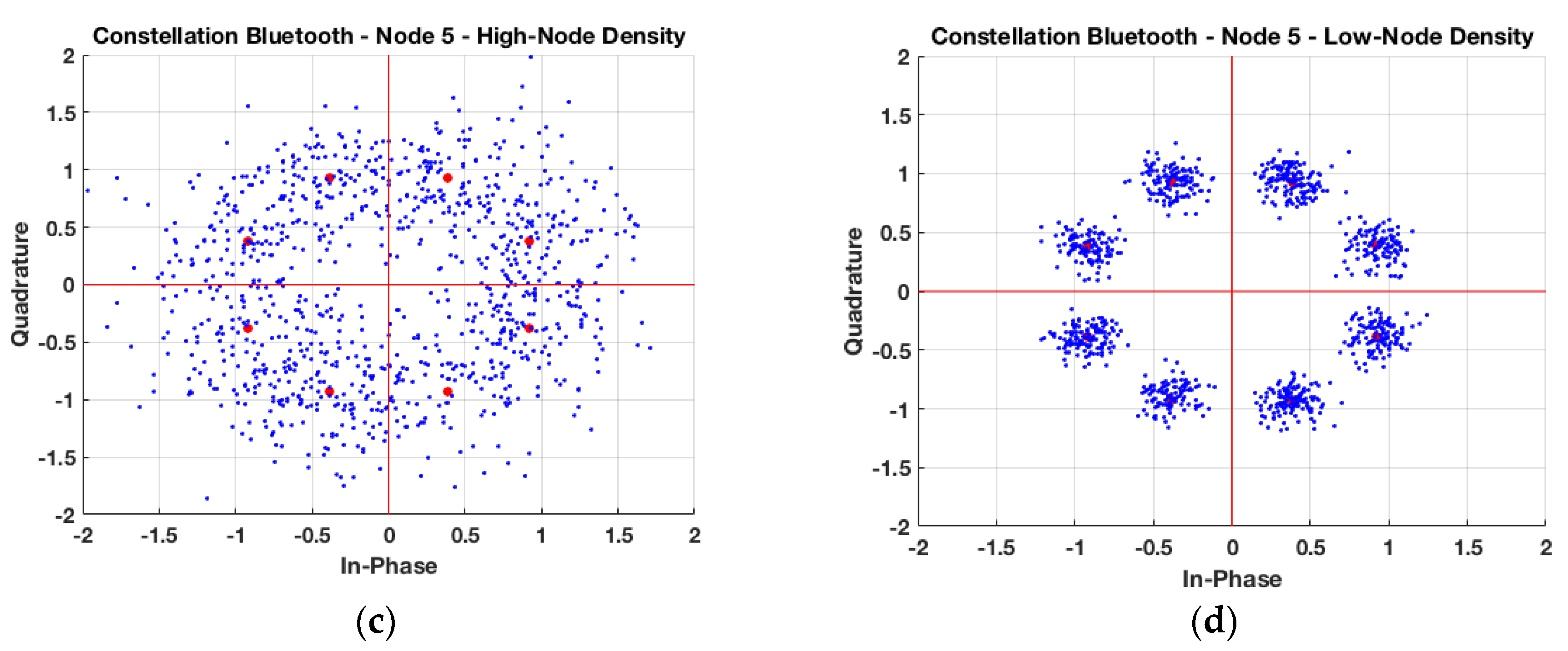
| System/Modulation/Bandwidth | ZigBee (2.4GHz)/O-QPSK/3 MHz Bluetooth V4.0/8-DPSK/2 MHz |
| Number of symbols | 1000 |
| RMS EVM (%) | High-Node Density | Medium-Node Density | Low-Node Density |
|---|---|---|---|
| Tx 33 (X = 20.35, Y = 22, Z = 1.2) m | 32.89 | 29.6 | 11.15 |
| Tx 5 (X = 11.7, Y = 3.8, Z = 1.2) m | 7.10 | 3.25 | 0.0022 |
| RMS EVM (%) | High-Node Density | Medium-Node Density | Low-Node Density |
|---|---|---|---|
| Tx 33 (X = 20.35, Y = 22, Z = 1.2) m | 47.61 | 46.39 | 27.24 |
| Tx 5 (X = 11.7, Y = 3.8, Z = 1.2) m | 28.66 | 11.19 | 3.06 |
© 2019 by the authors. Licensee MDPI, Basel, Switzerland. This article is an open access article distributed under the terms and conditions of the Creative Commons Attribution (CC BY) license (http://creativecommons.org/licenses/by/4.0/).
Share and Cite
Celaya-Echarri, M.; Azpilicueta, L.; López-Iturri, P.; Aguirre, E.; Falcone, F. Performance Evaluation and Interference Characterization of Wireless Sensor Networks for Complex High-Node Density Scenarios. Sensors 2019, 19, 3516. https://0-doi-org.brum.beds.ac.uk/10.3390/s19163516
Celaya-Echarri M, Azpilicueta L, López-Iturri P, Aguirre E, Falcone F. Performance Evaluation and Interference Characterization of Wireless Sensor Networks for Complex High-Node Density Scenarios. Sensors. 2019; 19(16):3516. https://0-doi-org.brum.beds.ac.uk/10.3390/s19163516
Chicago/Turabian StyleCelaya-Echarri, Mikel, Leyre Azpilicueta, Peio López-Iturri, Erik Aguirre, and Francisco Falcone. 2019. "Performance Evaluation and Interference Characterization of Wireless Sensor Networks for Complex High-Node Density Scenarios" Sensors 19, no. 16: 3516. https://0-doi-org.brum.beds.ac.uk/10.3390/s19163516