Selection of the Optimal Spectral Resolution for the Cadmium-Lead Cross Contamination Diagnosing Based on the Hyperspectral Reflectance of Rice Canopy


Abstract
:1. Introduction
2. Materials and Methods
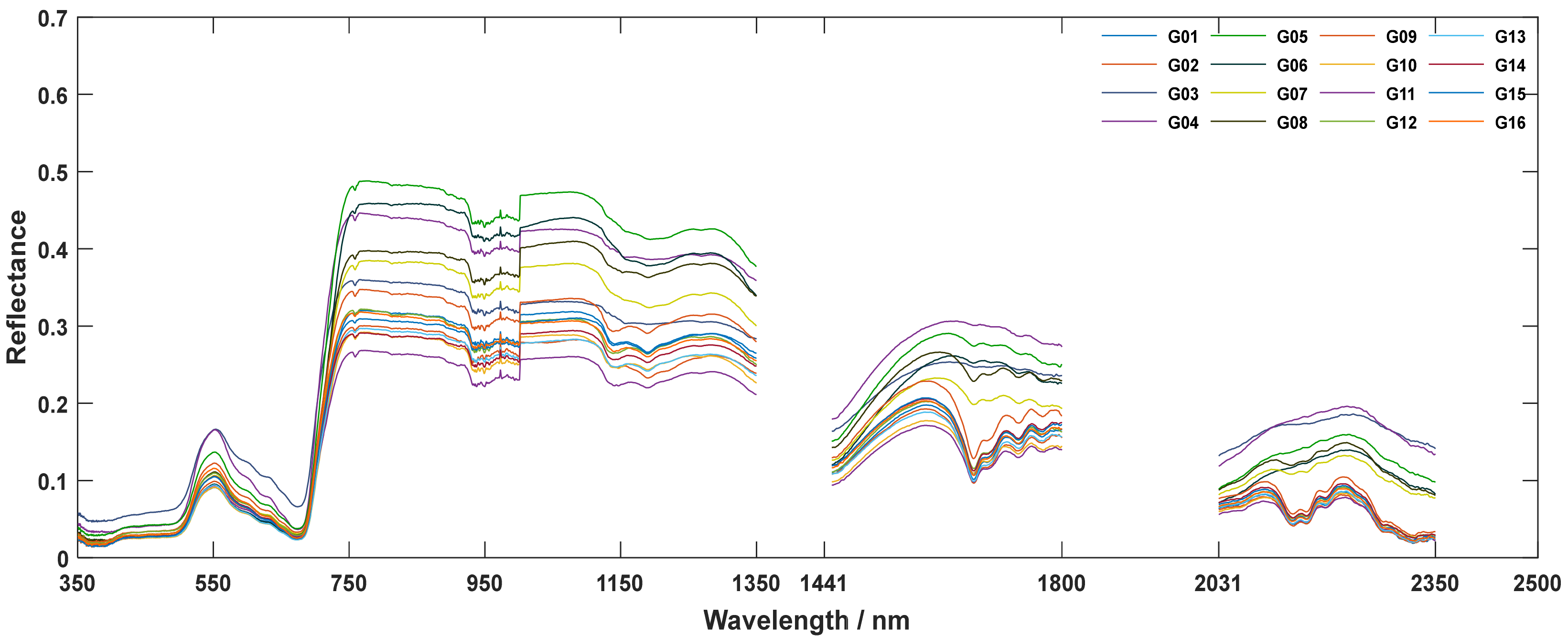
2.1. Materials
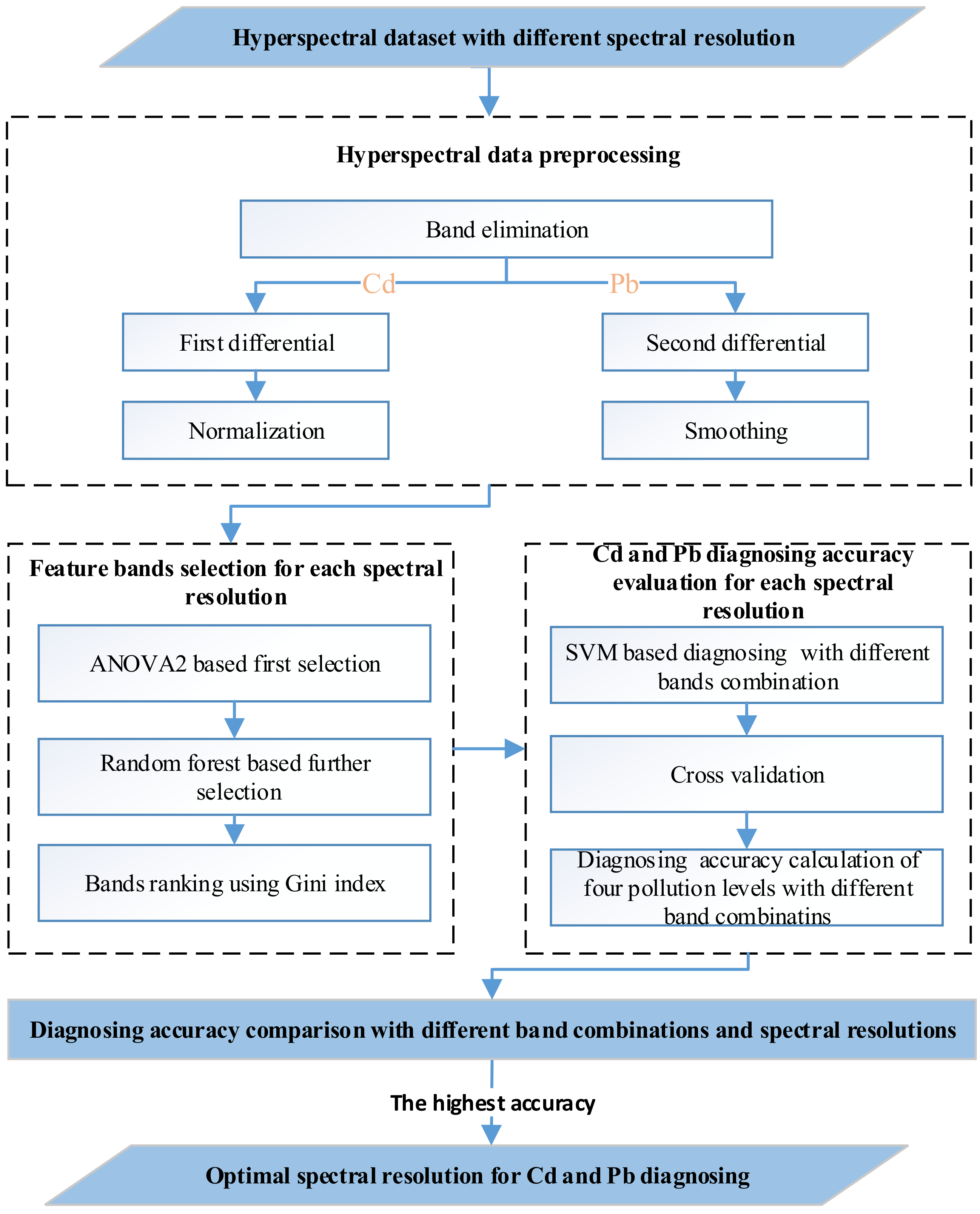
2.2. Methods
2.2.1. Hyperspectral Data Preprocessing
2.2.2. Feature Bands Selection
2.2.3. Cd and Pb Diagnosing and Accuracy Evaluation
2.2.4. Diagnosing Accuracy Comparison with Different Bands and Spectral Resolutions
3. Results
3.1. Results of Feature Bands Selection
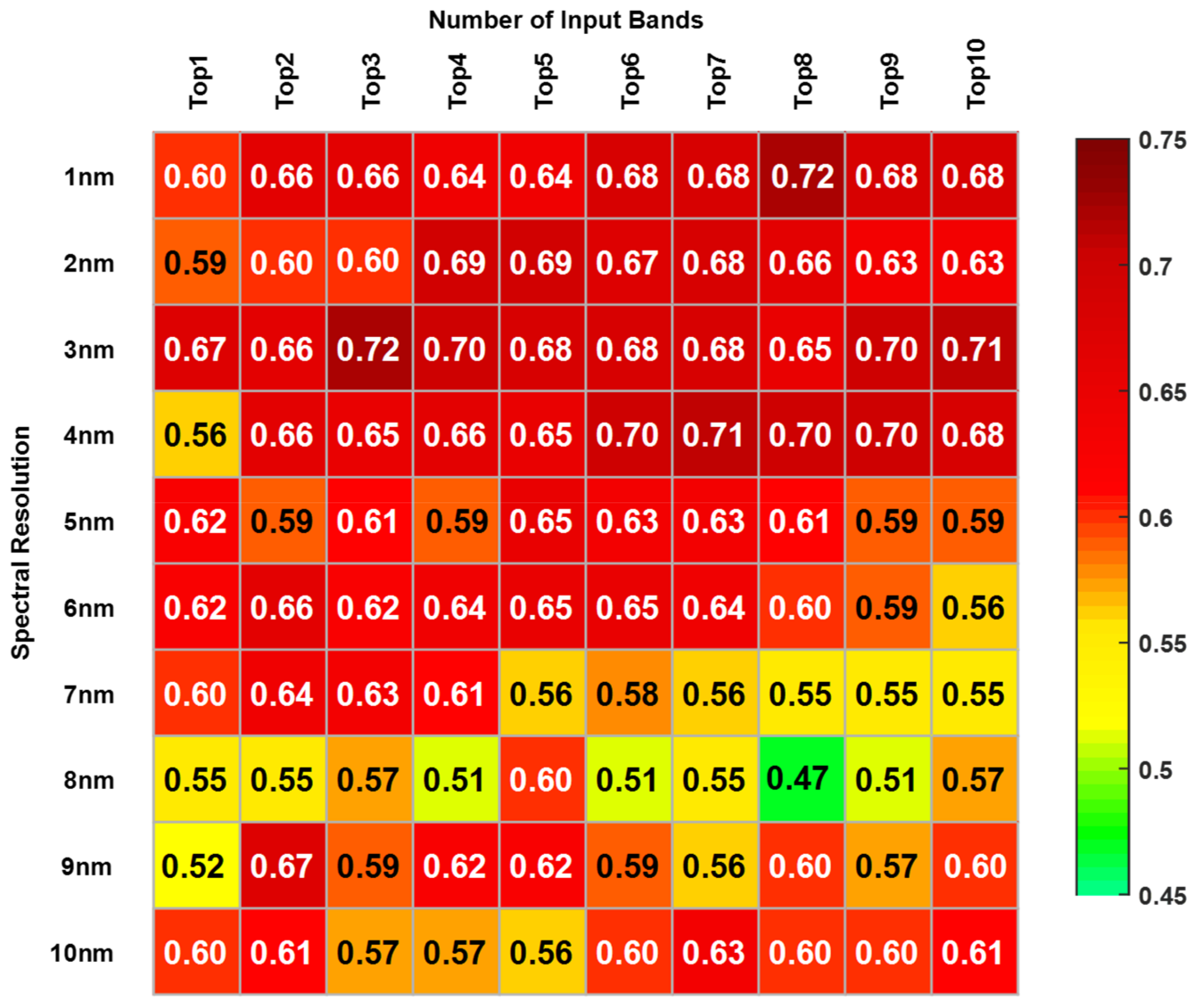
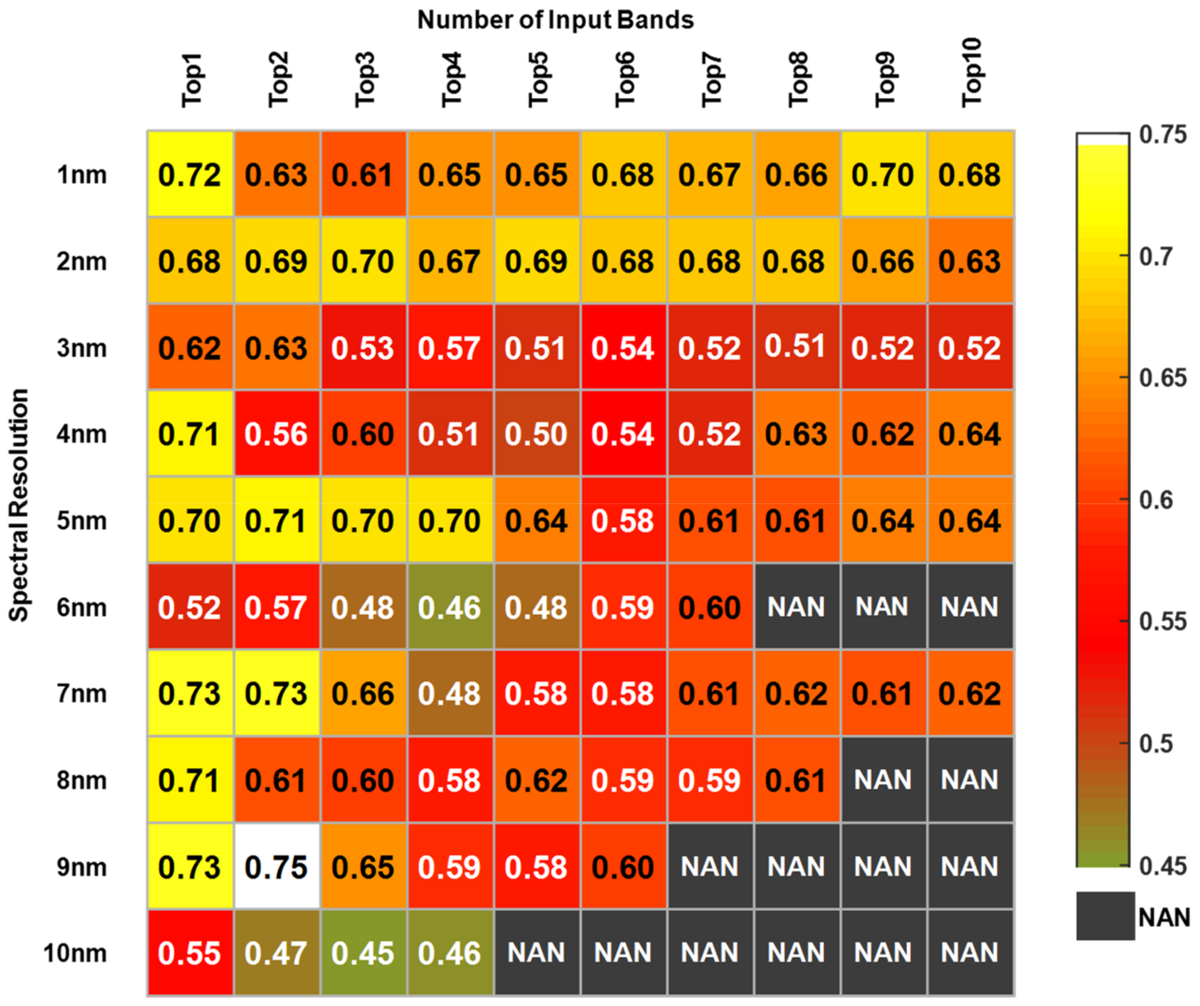
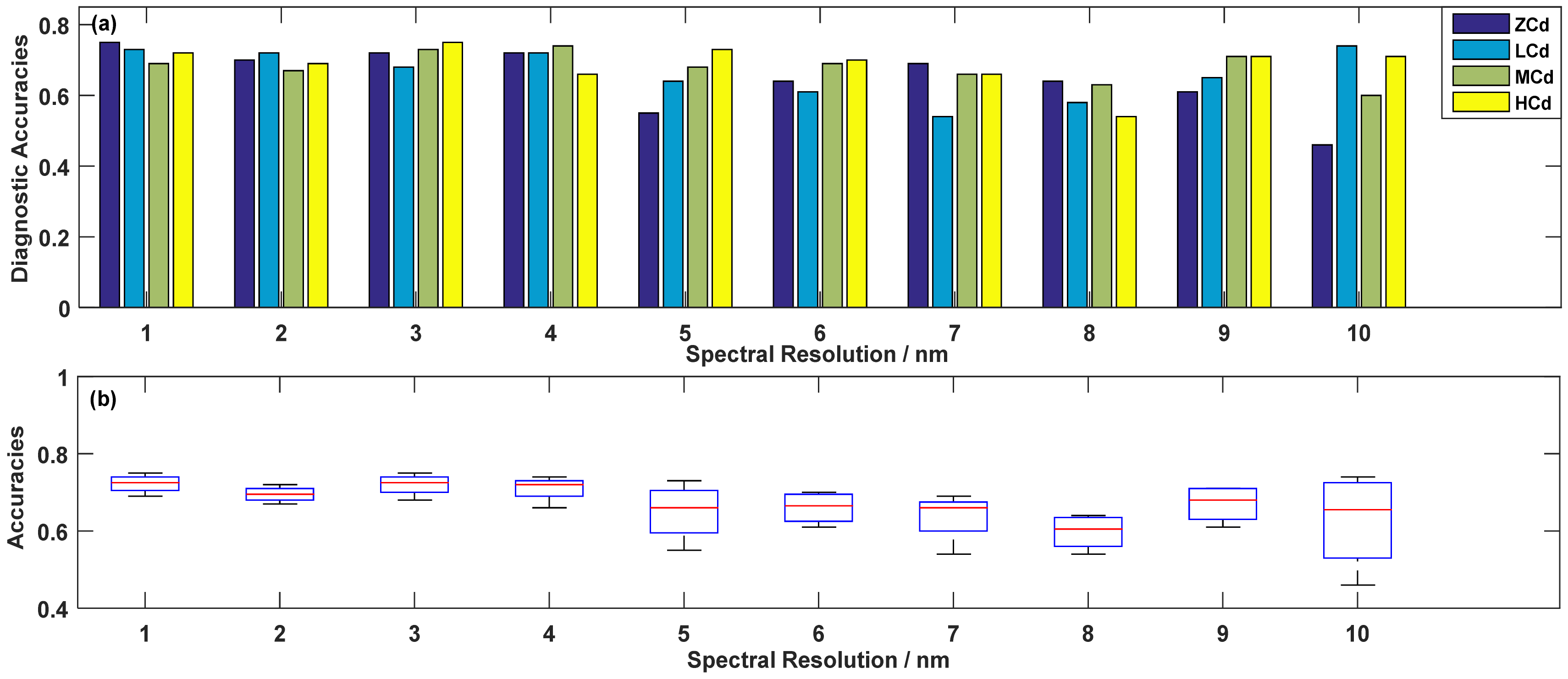
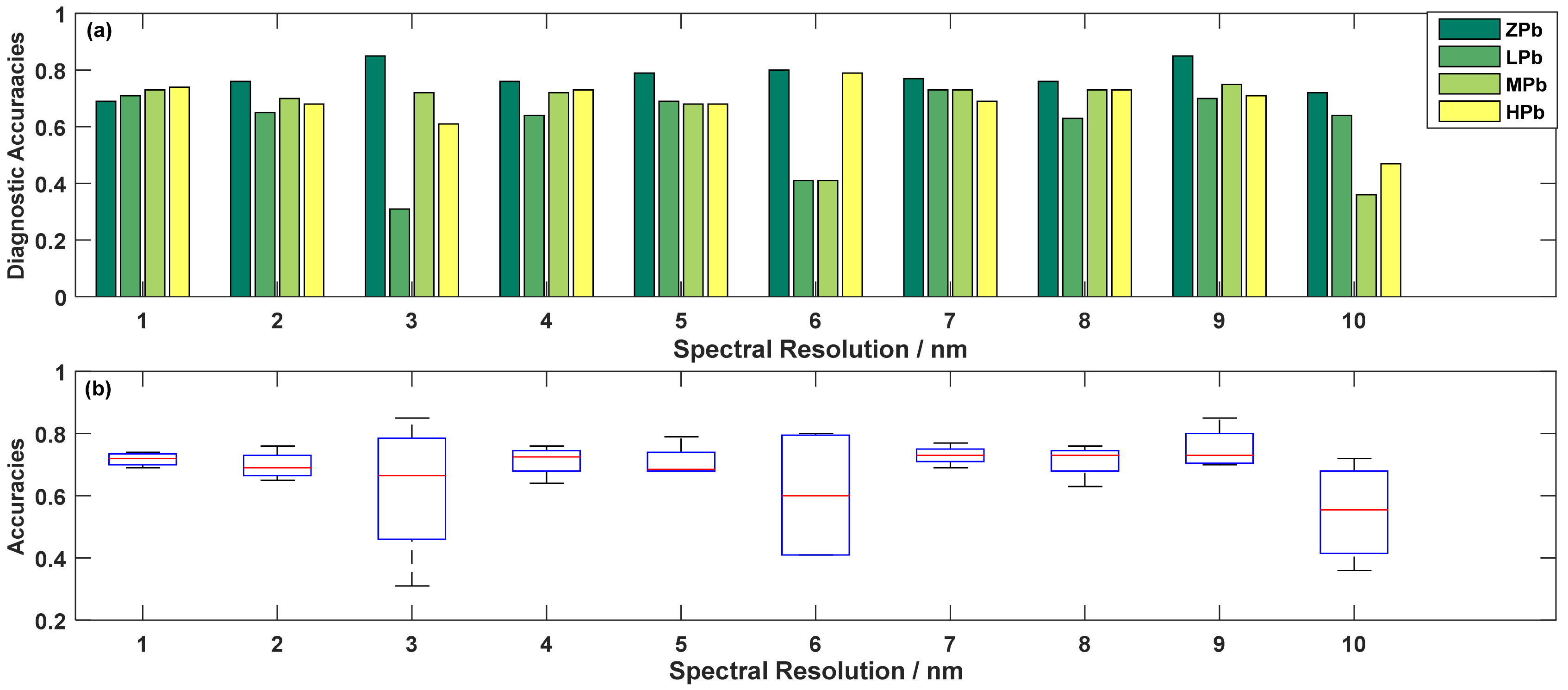
3.2. Diagnostic Accuracies of Different Spectral Resolution for Different Levels
4. Discussion
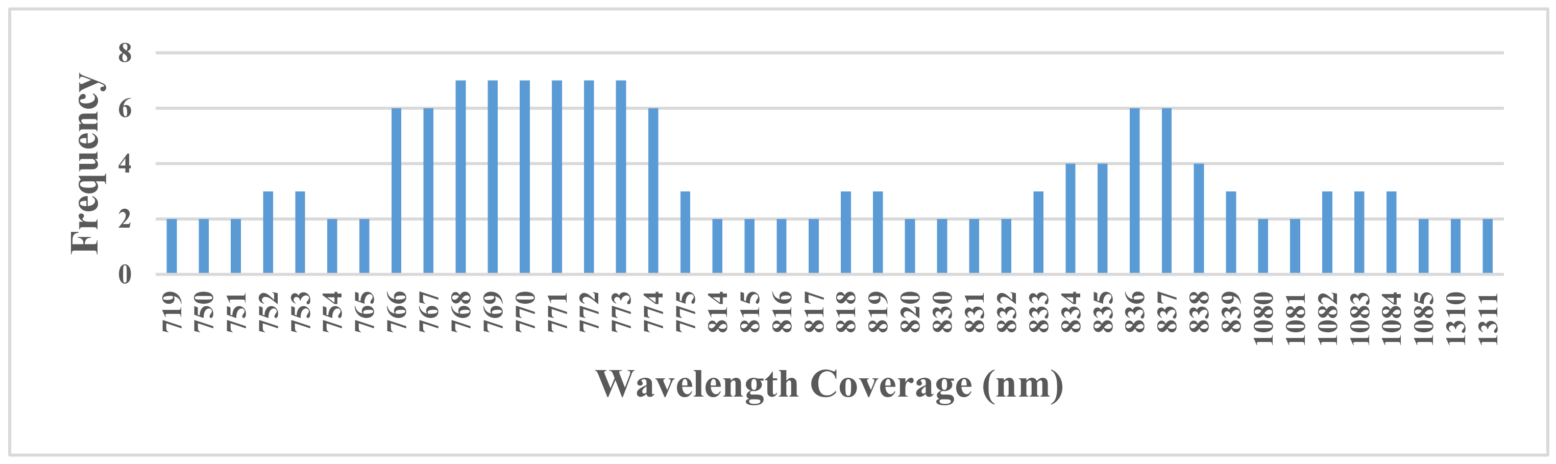
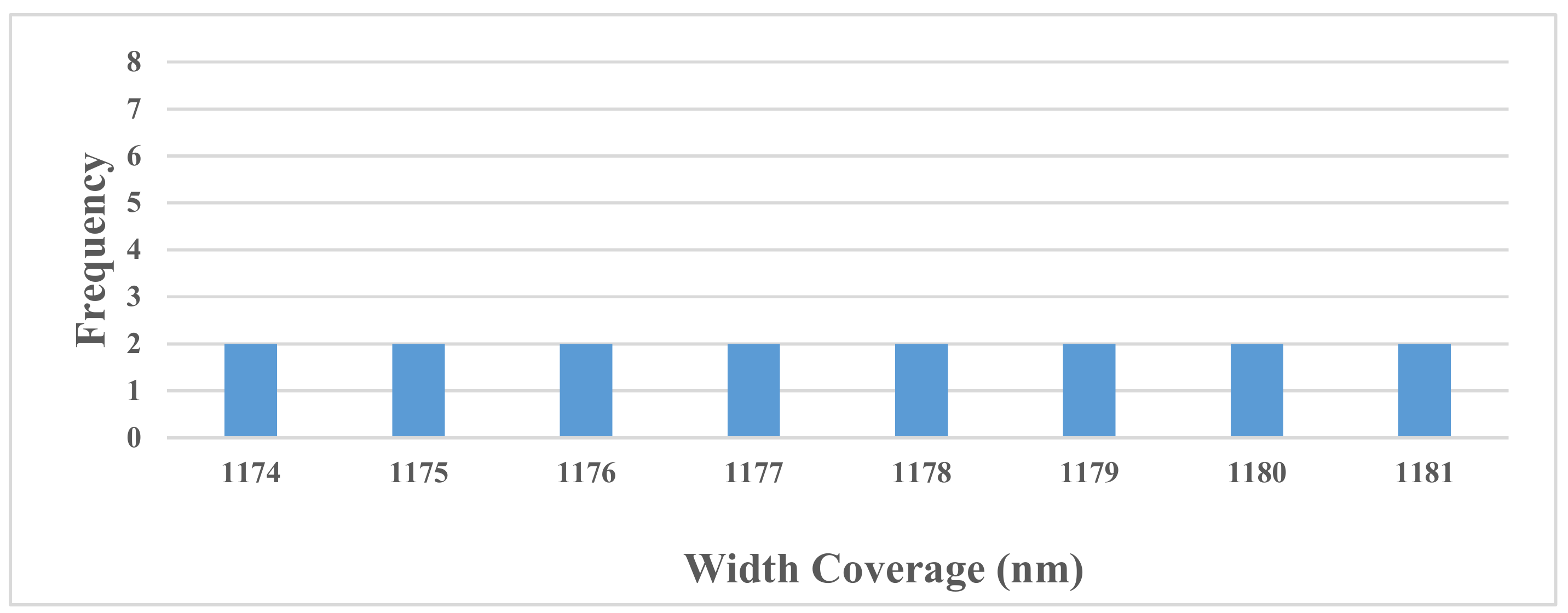
4.1. Suitable Wavelengths Analysis for Cd-Pb Pollution Diagnosing
4.2. Optimal Spectral Resolution Analysis
5. Conclusions
Author Contributions
Funding
Acknowledgments
Conflicts of Interest
References
- Khan, S.; Cao, Q.; Zheng, Y.M.; Huang, Y.Z.; Zhu, Y.G. Health risks of heavy metals in contaminated soils and food crops irrigated with wastewater in Beijing, China. Environ. Pollut. 2008, 152, 686–692. [Google Scholar] [CrossRef] [PubMed]
- Salazar, M.J.; Rodriguez, J.H.; Leonardo Nieto, G.; Pignata, M.L. Effects of heavy metal concentrations (Cd, Zn and Pb) in agricultural soils near different emission sources on quality, accumulation and food safety in soybean [Glycine max (L.) Merrill]. J. Hazard. Mater. 2012, 233, 244–253. [Google Scholar] [CrossRef] [PubMed]
- Leenaers, H.; Okx, J.P.; Burrough, P.A. Employing elevation data for efficient mapping of soil pollution on floodplains. Soil Use Manag. 1990, 6, 105–114. [Google Scholar]
- Steiger, B.V.; Webster, R.; Schulin, R.; Lehmann, R. Mapping heavy metals in polluted soil by disjunctive kriging. Environ. Pollut. 1996, 94, 205–215. [Google Scholar] [CrossRef]
- Huang, W.; Davidw, L.; Zheng, N.; Zhang, Y.; Liu, L.; Wang, J. Identification of yellow rust in wheat using in-situ spectral reflectance measurements and airborne hyperspectral imaging. Precis. Agric. 2007, 8, 187–197. [Google Scholar] [CrossRef]
- Wang, D.; Wilson, C.; Shannon, M.C. Interpretation of salinity and irrigation effects on soybean canopy reflectance in visible and near-infrared spectrum domain. Int. J. Remote Sens. 2002, 23, 811–824. [Google Scholar] [CrossRef]
- Rud, R.; Shoshany, M.; Alchanatis, V. Spectral indicators for salinity effects in crops: a comparison of a new green indigo ratio with existing indices. Remote Sens. Lett. 2010, 2, 289–298. [Google Scholar] [CrossRef]
- Shi, T.; Chen, Y.; Liu, Y.; Wu, G. Visible and near-infrared reflectance spectroscopy-an alternative for monitoring soil contamination by heavy metals. J. Hazard. Mater. 2014, 265, 166–176. [Google Scholar] [CrossRef] [PubMed]
- Liu, Y.; Li, W.; Wu, G.; Xu, X. Feasibility of estimating heavy metal contaminations in floodplain soils using laboratory-based hyperspectral data—A case study along Le’an River, China. Geosp. Inf. Sci. 2011, 14, 10–16. [Google Scholar] [CrossRef]
- Chen, T.; Chang, Q.; Clevers, J.G.; Kooistra, L. Rapid identification of soil cadmium pollution risk at regional scale based on visible and near-infrared spectroscopy. Environ. Pollut. 2015, 206, 217–226. [Google Scholar] [CrossRef] [PubMed]
- Shi, T.; Wang, J.; Chen, Y.; Wu, G. Improving the prediction of arsenic contents in agricultural soils by combining the reflectance spectroscopy of soils and rice plants. Int. J. Appl. Earth Obs. Geoinf. 2016, 52, 95–103. [Google Scholar] [CrossRef]
- Kooistra, L.; Wehrens, R.; Leuven, R.S.; Buydens, L.M. Possibilities of visible–near-infrared spectroscopy for the assessment of soil contamination in river floodplains. Anal. Chim. Acta 2001, 446, 97–105. [Google Scholar] [CrossRef]
- Malley, D.F.; Williams, P.C. Use of Near-Infrared Reflectance Spectroscopy in Prediction of Heavy Metals in Freshwater Sediment by Their Association with Organic Matter. Environ. Sci. Technol. 1997, 31, 3461–3467. [Google Scholar] [CrossRef]
- Moshou, D.; Bravoa, C.; Westb, J.; Wahlena, S.; Mccartneyb, A.; Ramona, H. Automatic Detection Of ‘Yellow Rust’ In Wheat Using Reflectance Measurements And Neural Networks. Comput. Electron. Agric. 2004, 44, 173–188. [Google Scholar] [CrossRef]
- Tilley, D.R.; Ahmed, M.; Son, J.H.; Badrinarayanan, H. Hyperspectral reflectance response of freshwater macrophytes to salinity in a brackish subtropical marsh. J. Environ. Qual. 2007, 36, 780–789. [Google Scholar] [CrossRef] [PubMed]
- St. Luce, M.; Ziadi, N.; Gagnon, B.; Karam, A. Visible near infrared reflectance spectroscopy prediction of soil heavy metal concentrations in paper mill biosolid- and liming by-product-amended agricultural soils. Geoderma 2017, 288, 23–36. [Google Scholar]
- Choe, E.; van der Meer, F.; van Ruitenbeek, F.; van der Werff, H.; de Smeth, B.; Kim, K.-W. Mapping of heavy metal pollution in stream sediments using combined geochemistry, field spectroscopy, and hyperspectral remote sensing: A case study of the Rodalquilar mining area, SE Spain. J. Environ. Qual. 2008, 112, 3222–3233. [Google Scholar] [CrossRef]
- Wang, J.; Cui, L.; Gao, W.; Shi, T.; Chen, Y.; Gao, Y. Prediction of low heavy metal concentrations in agricultural soils using visible and near-infrared reflectance spectroscopy. Geoderma 2014, 216, 1–9. [Google Scholar] [CrossRef]
- Liu, M.; Liu, X.; Ding, W.; Wu, L. Monitoring stress levels on rice with heavy metal pollution from hyperspectral reflectance data using wavelet-fractal analysis. Int. J. Appl. Earth Obs. Geoinf. 2011, 13, 246–255. [Google Scholar] [CrossRef]
- Vandermeulen, R.A.; Mannino, A.; Neeley, A.; Werdell, J.; Arnone, R. Determining the optimal spectral sampling frequency and uncertainty thresholds for hyperspectral remote sensing of ocean color. Opt. Express 2017, 25, A785–A797. [Google Scholar] [CrossRef]
- Nidamanuri, R.R.; Zbell, B. A method for selecting optimal spectral resolution and comparison metric for material mapping by spectral library search. Prog. Phys. Geog. 2010, 34, 47–58. [Google Scholar] [CrossRef]
- Dalponte, M.; Bruzzone, L.; Vescovo, L.; Gianelle, D. The role of spectral resolution and classifier complexity in the analysis of hyperspectral images of forest areas. Remote Sens. Environ. 2009, 113, 2345–2355. [Google Scholar] [CrossRef]
- Hughes, G.P. On the mean accuracy of statistical pattern recognizers. IEEE Trans. Inf. Theory 1968, 14, 55–63. [Google Scholar] [CrossRef]
- Fu, J.; Zhou, Q.; Liu, J.; Liu, W.; Wang, T.; Zhang, Q.; Jiang, G. High levels of heavy metals in rice (Oryza sativa L.) from a typical E-waste recycling area in southeast China and its potential risk to human health. Chemosphere 2008, 71, 1269–1275. [Google Scholar] [PubMed]
- Gao, W.; Whiting, M.L.; Jackson, T.J. Measuring surface water in soil with light reflectance. Int. Soc. Opt. Photonics 2009, 7454, 74540D. [Google Scholar]
- MEE; SAMR. Risk Control Standard for Soil Contamination of Agricultural Land; GB15618-2018; Standards Press of China Beijing: Beijing, China, 2018; pp. 1–10. (In Chinese) [Google Scholar]
- Jiang, Q.; Liu, M.; Wang, J.; Liu, F. Feasibility of using visible and near-infrared reflectance spectroscopy to monitor heavy metal contaminants in urban lake sediment. Catena 2018, 162, 72–79. [Google Scholar] [CrossRef]
- Kooistra, L.; Salas, E.A.L.; Clevers, J.G.P.W.; Wehrens, R.; Leuven, R.S.E.W.; Nienhuis, P.H.; Buydens, L.M.C. Exploring field vegetation reflectance as an indicator of soil contamination in river floodplains. Environ. Pollut. 2004, 127, 281–290. [Google Scholar] [CrossRef]
- Kemper, T.; Ehlers, M.; Sommer, S.; Posa, F.; Kaufmann, H.J.; Michel, U.; De Carolis, G. Use of airborne hyperspectral data to estimate residual heavy metal contamination and acidification potential in the Guadiamar floodplain Andalusia, Spain after the Aznacollar mining accident. Int. Soc. Opt. Photonics 2004, 5574, 224–234. [Google Scholar]
- Wang, T.; Wei, H.; Zhou, C.; Gu, Y.; Li, R.; Chen, H.; Ma, W. Estimating cadmium concentration in the edible part of Capsicum annuum using hyperspectral models. Environ. Monit. Assess. 2017, 189, 548. [Google Scholar] [CrossRef]
- Sridhar, B.B.M.; Vincent, R.K.; Roberts, S.J.; Czajkowski, K. Remote sensing of soybean stress as an indicator of chemical concentration of biosolid amended surface soils. Int. J. Appl. Earth Obs. Geoinf. 2011, 13, 676–681. [Google Scholar] [CrossRef]
- Maanan, M.; Saddik, M.; Maanan, M.; Chaibi, M.; Assobhei, O.; Zourarah, B. Environmental and ecological risk assessment of heavy metals in sediments of Nador lagoon, Morocco. Ecol. Indic. 2015, 48, 616–626. [Google Scholar] [CrossRef]
- Jin, X.; Du, J.; Liu, H.; Wang, Z.; Song, K. Remote estimation of soil organic matter content in the Sanjiang Plain, Northest China: The optimal band algorithm versus the GRA-ANN model. Agric. For. Meteorol. 2016, 218, 250–260. [Google Scholar] [CrossRef]
- Martens, H.E.; Naes, T. Multivariate Calibration. Biometrics 1989, 47, 380–395. [Google Scholar]
- Savitzky, A.; Golay, M.J.E. Smoothing and Differentiation of Data by Simplified Least Squares Procedures. Anal. Chem. 1964, 36, 1627–1639. [Google Scholar] [CrossRef]
- Wang, D.; Liu, X. Comparative Analysis of GF-1 and HJ-1 Data to Derive the Optimal Scale for Monitoring Heavy Metal Stress in Rice. Int. J. Environ. Res. Public Health 2018, 15, 461. [Google Scholar] [CrossRef] [PubMed]
- Lu, H.; Yu, X.; Zhou, L.; He, Y. Selection of Spectral Resolution and Scanning Speed for Detecting Green Jujubes Chilling Injury Based on Hyperspectral Reflectance Imaging. Appl. Sci. 2018, 8, 523. [Google Scholar] [CrossRef]
- Marceau, D.J.; Hay, G.J. Remote Sensing Contributions to the Scale Issue. Can. J. Remote Sens. 1999, 25, 357–366. [Google Scholar] [CrossRef]


| Group Name | Pollution Pretreatment | Group Name | Pollution Pretreatment |
|---|---|---|---|
| G01 | ZCd-ZPb | G09 | LCd-MPb |
| G02 | LCd-ZPb | G10 | LCd-HPb |
| G03 | MCd-ZPb | G11 | MCd-LPb |
| G04 | HCd-ZPb | G12 | MCd-MPb |
| G05 | ZCd-LPb | G13 | MCd-HPb |
| G06 | ZCd-MPb | G14 | HCd-LPb |
| G07 | ZCd-HPb | G15 | HCd-MPb |
| G08 | LCd-LPb | G16 | HCd-HPb |
| Spectral Resolution | Primitive Bands | Cd | Pb | ||
|---|---|---|---|---|---|
| Bands after ANOVA2 | Input Bands after RF | Bands after ANOVA2 | Input Bands after RF | ||
| 1 nm | 1660 | 48 | 8 | 50 | 1 |
| 2 nm | 830 | 34 | 4 | 31 | 3 |
| 3 nm | 552 | 26 | 3 | 20 | 2 |
| 4 nm | 415 | 28 | 7 | 11 | 1 |
| 5 nm | 332 | 23 | 5 | 14 | 2 |
| 6 nm | 275 | 21 | 2 | 7 | 7 |
| 7 nm | 235 | 19 | 2 | 14 | 1 |
| 8 nm | 207 | 17 | 5 | 8 | 1 |
| 9 nm | 183 | 19 | 2 | 6 | 2 |
| 10 nm | 166 | 12 | 7 | 4 | 1 |
| ZCd | LCd | MCd | HCd | ZPb | LPb | MPb | HPb | |
|---|---|---|---|---|---|---|---|---|
| 1 nm | 0.75 | 0.73 | 0.69 | 0.72 | 0.69 | 0.71 | 0.73 | 0.74 |
| 2 nm | 0.70 | 0.72 | 0.67 | 0.69 | 0.76 | 0.65 | 0.70 | 0.68 |
| 3 nm | 0.72 | 0.68 | 0.73 | 0.75 | 0.85 | 0.31 | 0.72 | 0.61 |
| 4 nm | 0.72 | 0.72 | 0.74 | 0.66 | 0.76 | 0.64 | 0.72 | 0.73 |
| 5 nm | 0.55 | 0.64 | 0.68 | 0.73 | 0.79 | 0.69 | 0.68 | 0.68 |
| 6 nm | 0.64 | 0.61 | 0.69 | 0.70 | 0.80 | 0.41 | 0.41 | 0.79 |
| 7 nm | 0.69 | 0.54 | 0.66 | 0.66 | 0.77 | 0.73 | 0.73 | 0.69 |
| 8 nm | 0.64 | 0.58 | 0.63 | 0.54 | 0.76 | 0.63 | 0.73 | 0.73 |
| 9 nm | 0.61 | 0.65 | 0.71 | 0.71 | 0.85 | 0.70 | 0.75 | 0.71 |
| 10 nm | 0.46 | 0.74 | 0.60 | 0.71 | 0.72 | 0.64 | 0.36 | 0.47 |
| Spectral Resolution | Band Width |
|---|---|
| 1 nm | 734 nm, 754–755 nm, 768–769 nm, 776 nm, 1237 nm, 1309 nm, 1831 nm |
| 2 nm | 766–773 nm, 1310–1311 nm |
| 3 nm | 719–721 nm, 752–754 nm, 767–775 nm, 818–820 nm, 836–838 nm, 1214–1216 nm, 1310–1312 nm |
| 4 nm | 382–385 nm, 750–753 nm, 766–773 nm, 834–837 nm, 1082–1085 nm, 1298–1301 nm |
| 5 nm | 765–774 nm, 785–789 nm, 1015–1019 nm, 1080–1084 nm |
| 6 nm | 764–775 nm |
| 7 nm | 770–776 nm, 833–839 nm |
| 8 nm | 766–773 nm, 814–821 nm, 830–837 nm, 1078–1085 nm, 1222–1229 nm |
| 9 nm | 746–754 nm, 836–844 nm |
| 10 nm | 710–719 nm, 810–819 nm, 830–839 nm, 1020–1029 nm, 1310–1319 nm, 1340–1349 nm |
| Spectral Resolution | Band Width |
|---|---|
| 1 nm | 761 nm |
| 2 nm | 708–709 nm, 762–763 nm |
| 3 nm | 638–640 nm, 884–886 nm |
| 4 nm | 1174–1177 nm |
| 5 nm | 765–769 nm, 1891–1895 nm |
| 6 nm | 392–397 nm, 467–481 nm, 518–529 nm, 572–577 nm, 614–619 nm, 1394–1399 nm |
| 7 nm | 1771–1777 nm |
| 8 nm | 1174–1181 nm |
| 9 nm | 1178–1186 nm, 1870–1878 nm |
| 10 nm | 920–929 nm |
| Spectral Resolution | 1 nm | 2 nm | 3 nm | 4 nm | 5 nm | 6 nm | 7 nm | 8 nm | 9 nm | 10 nm |
|---|---|---|---|---|---|---|---|---|---|---|
| AV | 0.69 | 0.69 | 0.65 | 0.66 | 0.66 | 0.62 | 0.68 | 0.63 | 0.71 | 0.57 |
| Standard Deviation | 0.11 | 0.03 | 0.1 | 0.12 | 0.07 | 0.14 | 0.06 | 0.19 | 0.07 | 0.12 |
| Recall Ratio | 0.83 | 0.75 | 0.69 | 0.59 | 0.79 | 0.61 | 0.75 | 0.80 | 0.76 | 0.61 |
| Range | 0.40 | 0.13 | 0.35 | 0.43 | 0.23 | 0.41 | 0.23 | 0.55 | 0.24 | 0.35 |
| Variable Coefficient | 0.16 | 0.05 | 0.16 | 0.18 | 0.10 | 0.22 | 0.09 | 0.30 | 0.09 | 0.21 |
© 2019 by the authors. Licensee MDPI, Basel, Switzerland. This article is an open access article distributed under the terms and conditions of the Creative Commons Attribution (CC BY) license (http://creativecommons.org/licenses/by/4.0/).
Share and Cite
Zhang, S.; Zhu, Y.; Wang, M.; Fei, T. Selection of the Optimal Spectral Resolution for the Cadmium-Lead Cross Contamination Diagnosing Based on the Hyperspectral Reflectance of Rice Canopy. Sensors 2019, 19, 3889. https://0-doi-org.brum.beds.ac.uk/10.3390/s19183889
Zhang S, Zhu Y, Wang M, Fei T. Selection of the Optimal Spectral Resolution for the Cadmium-Lead Cross Contamination Diagnosing Based on the Hyperspectral Reflectance of Rice Canopy. Sensors. 2019; 19(18):3889. https://0-doi-org.brum.beds.ac.uk/10.3390/s19183889
Chicago/Turabian StyleZhang, Shuangyin, Ying Zhu, Mi Wang, and Teng Fei. 2019. "Selection of the Optimal Spectral Resolution for the Cadmium-Lead Cross Contamination Diagnosing Based on the Hyperspectral Reflectance of Rice Canopy" Sensors 19, no. 18: 3889. https://0-doi-org.brum.beds.ac.uk/10.3390/s19183889