Cross-Category Tea Polyphenols Evaluation Model Based on Feature Fusion of Electronic Nose and Hyperspectral Imagery

 , ,
, , 
Abstract
:
1. Background
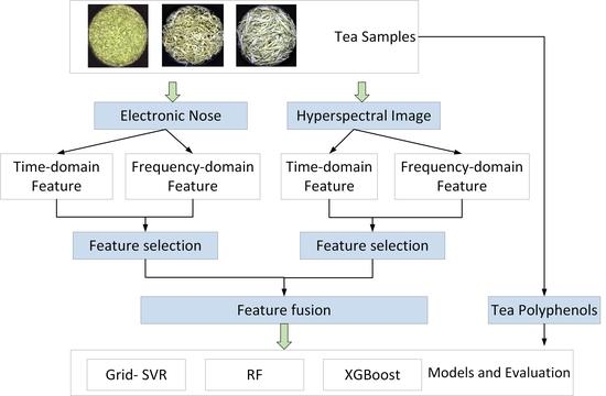
2. Data and Methods
2.1. Sample Collection
2.2. Sample Sampling
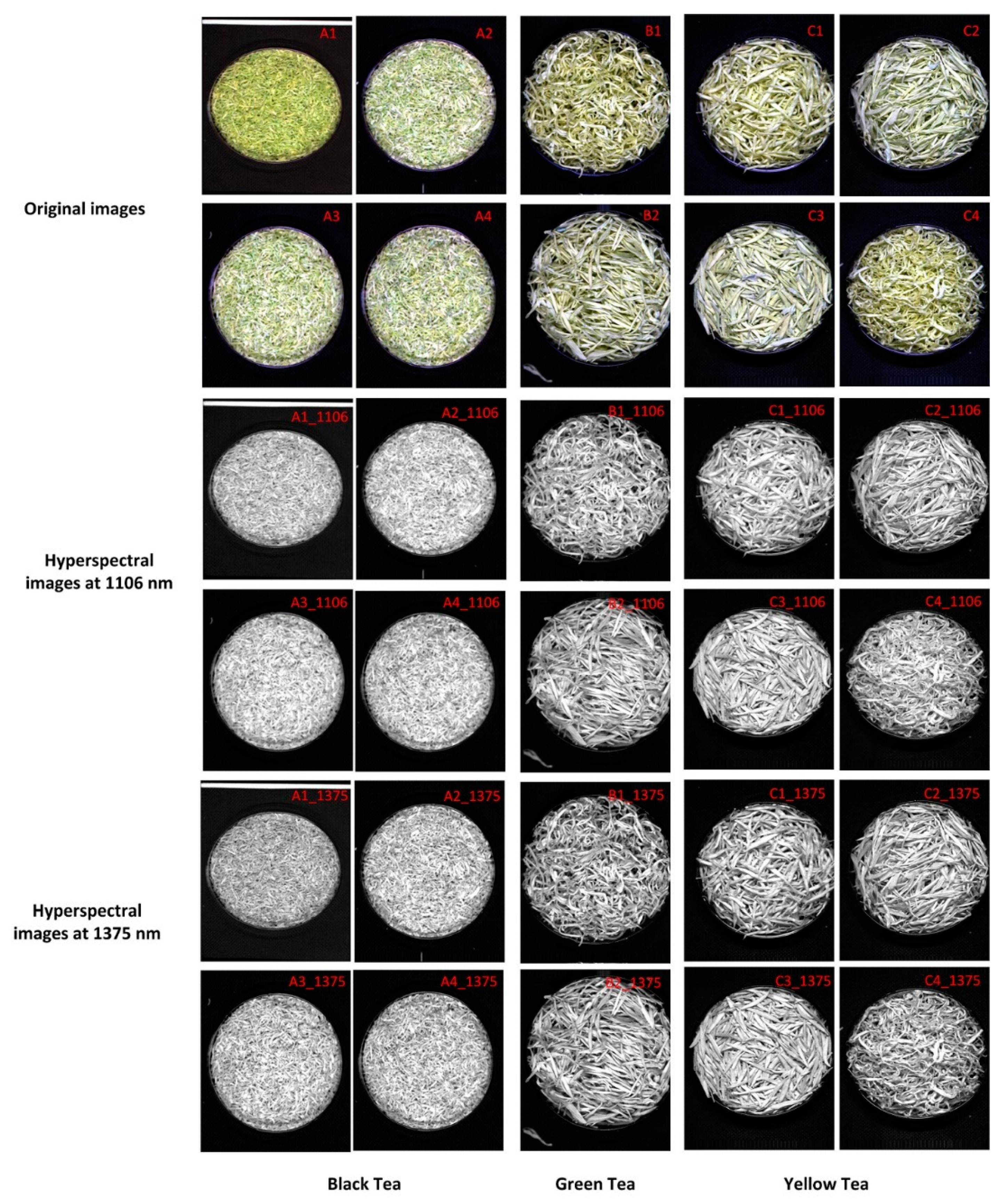
2.2.1. HSI Sampling
2.2.2. E-Nose Sampling
2.3. Feature Extraction
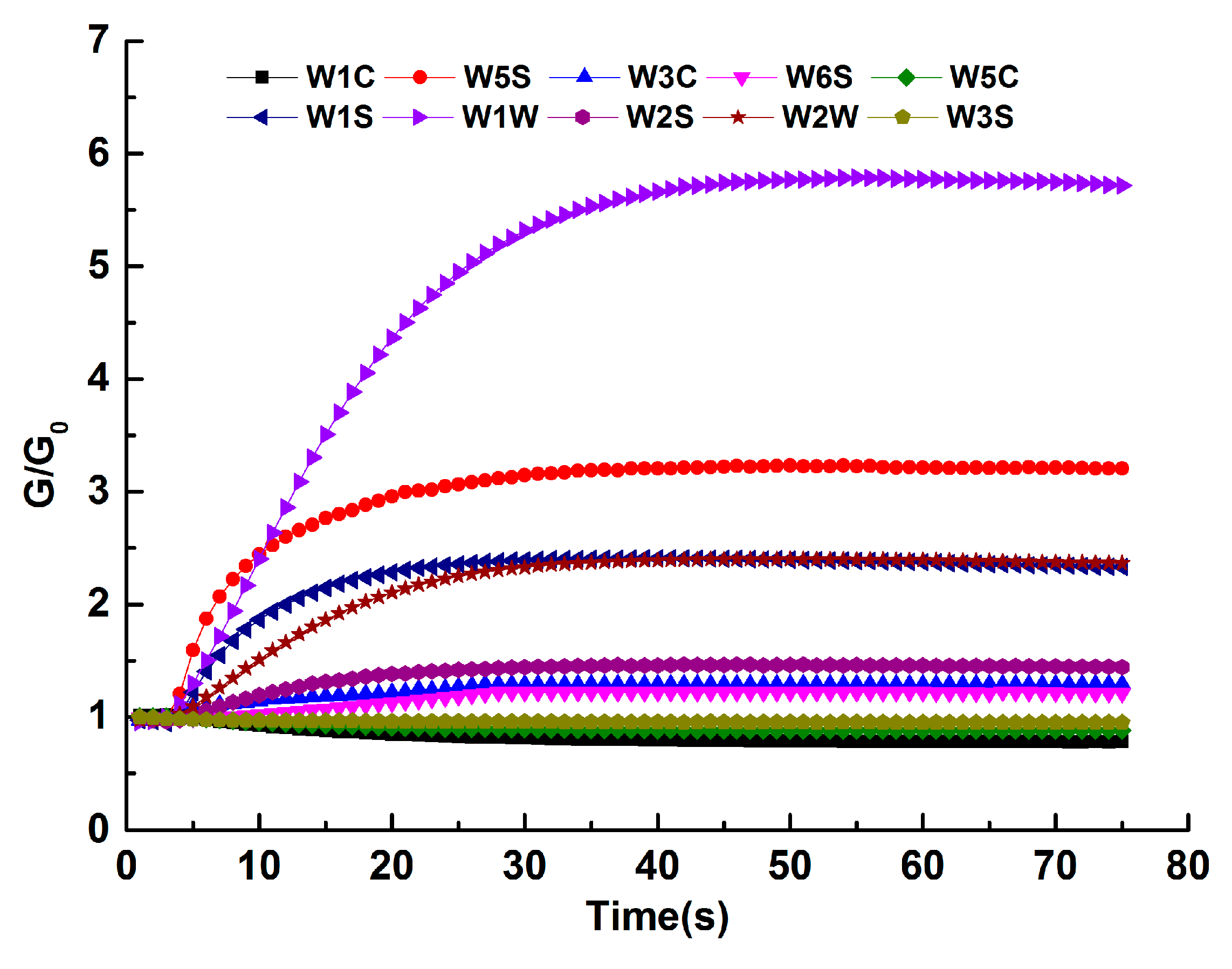
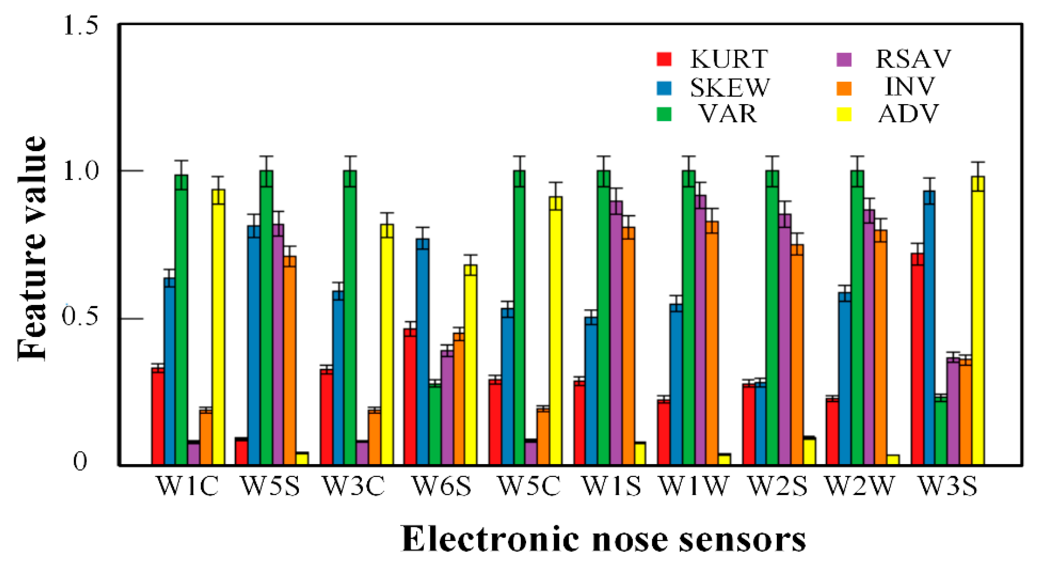
2.3.1. Feature Extraction from E-Nose System
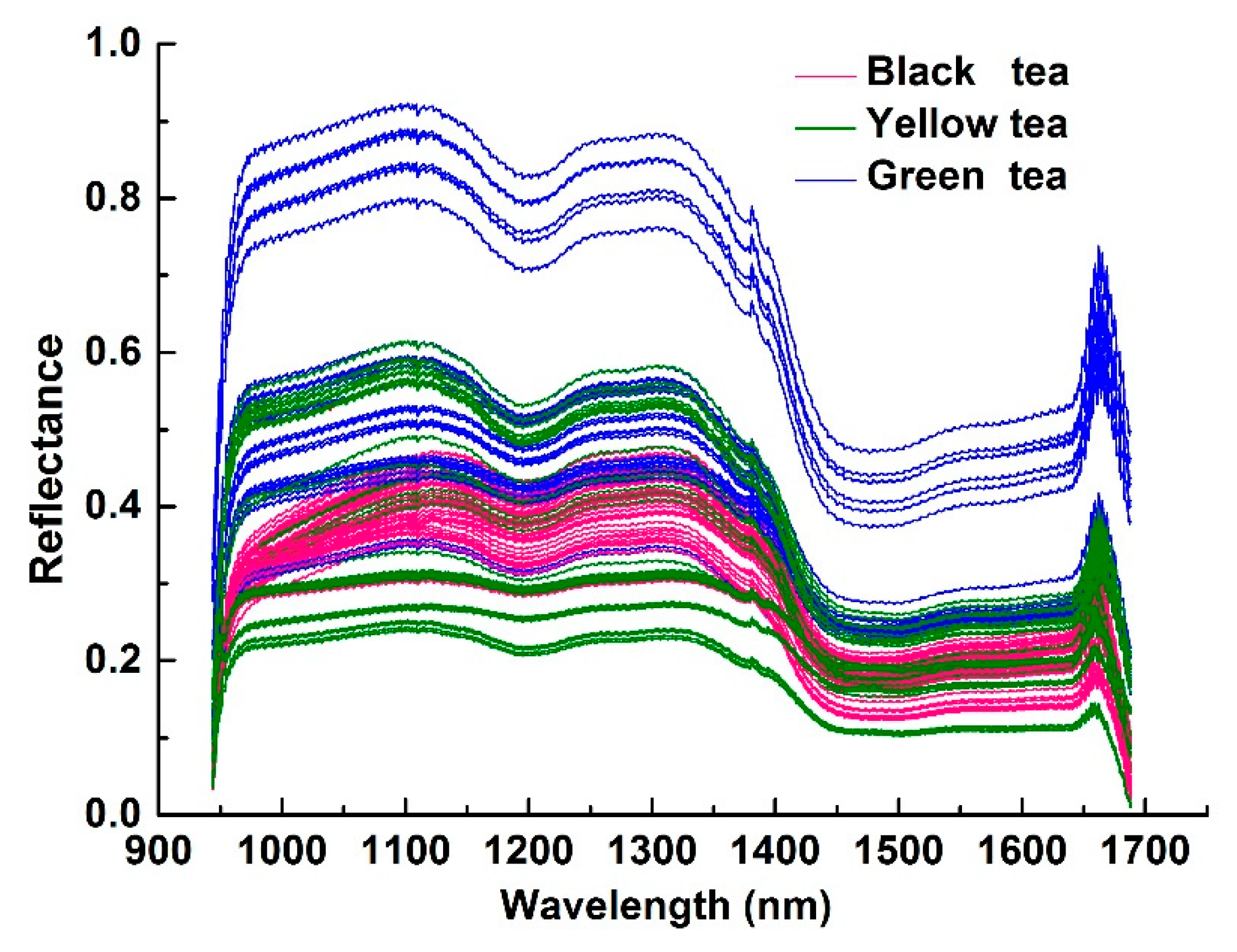
2.3.2. Feature Extraction from HSI
2.4. Methodology
2.4.1. Normalized Processing
2.4.2. Support Vector Regression
2.4.3. Random Forest
2.4.4. Extreme Gradient Boosting
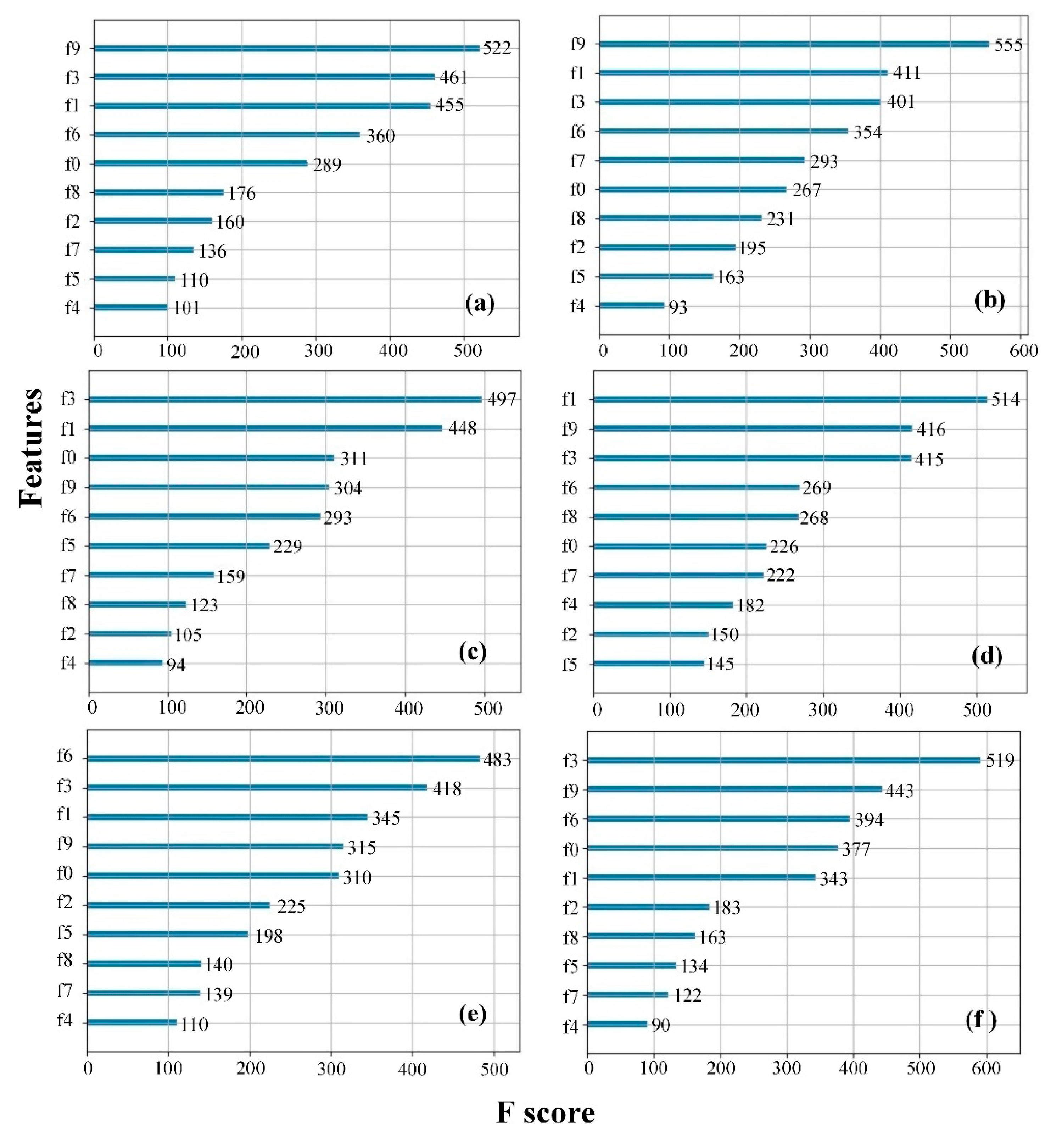
2.4.5. Feature Importance Assessment Method
3. Results and Analysis
3.1. Feature Extraction and Feature Selection from E-Nose System
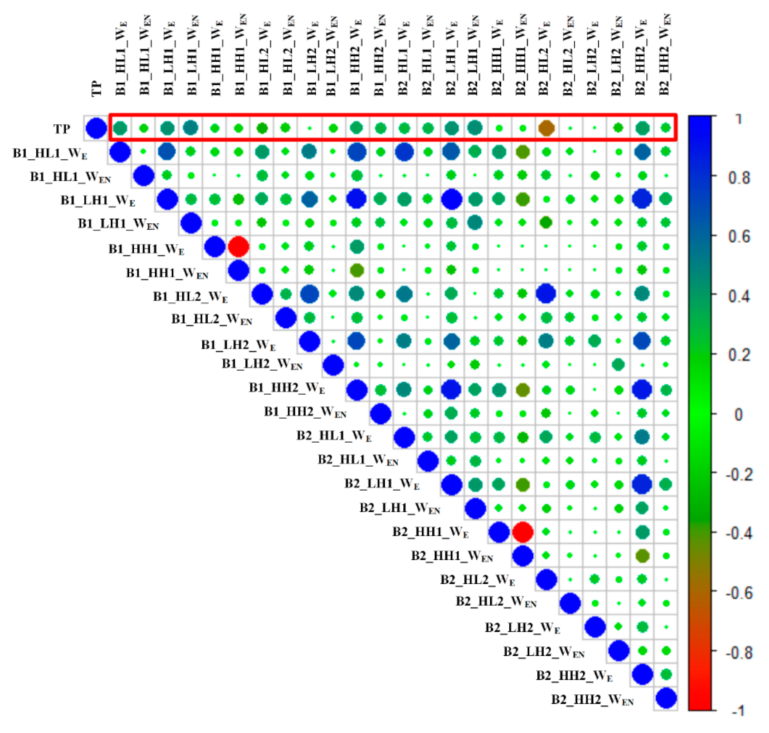
3.2. Feature Extraction and Feature Selection from HSI
3.3. Different Methods for Estimation of Polyphenol Content in Cross-Category Tea
3.4. Results of Models Based on Different Features
4. Discussion
4.1. Wavelet Transform and Features
4.2. Different Features Affect Estimation Results
4.3. Different Regression Models Affect Estimation Results
5. Conclusions
Author Contributions
Funding
Conflicts of Interest
References
- Alexandr, Y.; Boris, V.; Emilie, C.; Yakov, I. Determination of the chemical composition of tea by chromatographic methods: A review. J. Food Res. 2015, 4, 56–88. [Google Scholar]
- Juneja, L.; Chu, D.; Okubo, T.; Nagato, Y.; Yokogoshi, H. L-theanine—A unique amino acid of green tea and its relaxation effect in humans. Trends Food Sci. Technol. 1999, 10, 199–204. [Google Scholar] [CrossRef]
- Qian, Y.; Zhang, S.; Yao, S.; Xia, J.; Li, Y.; Dai, X.; Wang, W.; Jiang, X.; Liu, Y.; Li, M.; et al. Effects of vitro sucrose on quality components of tea plants (Camellia sinensis) based on transcriptomic and metabolic analysis. BMC Plant Biol. 2018, 18, 121. [Google Scholar] [CrossRef] [PubMed]
- Jia, W.; Liang, G.; Jiang, Z.; Wang, J. Advances in Electronic Nose Development for Application to Agricultural Products. Food Anal. Meth. 2019, 12, 2226–2240. [Google Scholar] [CrossRef]
- Nishitani, E.; Sagesaka, Y.M. Simultaneous determination of catechins, caffeine and other phenolic compounds in tea using new HPLC method. J. Food Compos. Anal. 2004, 17, 675–685. [Google Scholar] [CrossRef]
- Togari, N.; Kobayashi, A.; Aishima, T. Pattern recognition applied to gas chromatographic profiles of volatile components in three tea categories. Food Res. Int. 1995, 28, 495–502. [Google Scholar] [CrossRef]
- Kotani, A.; Takahashi, K.; Hakamata, H.; Kojima, S.; Kusu, F. Attomole catechins determination by capillary liquid chromatography with electrochemical detection. Anal. Sci. 2007, 23, 157–163. [Google Scholar] [CrossRef] [Green Version]
- Lee, M.; Hwang, Y.; Lee, J.; Choung, M. The characterization of caffeine and nine individual catechins in the leaves of green tea (Camellia sinensis L.) by near-infrared reflectance spectroscopy. Food Chem. 2014, 158, 351–357. [Google Scholar] [CrossRef]
- Ren, G.; Wang, S.; Ning, J.; Xu, R.; Wang, Y.; Xing, Z.; Wan, X.; Zhang, Z. Quantitative analysis and geographical traceability of black tea using Fourier transform near-infrared spectroscopy (FT-NIRS). Food Res. Int. 2013, 53, 822–826. [Google Scholar] [CrossRef]
- Chen, G.; Yuan, Q.; Saeeduddin, M.; Ou, S.; Zeng, X.; Ye, H. Recent advances in tea polysaccharides: Extraction, purification, physicochemical characterization and bioactivities. Carbohydr. Polym. 2016, 153, 663–678. [Google Scholar] [CrossRef]
- Sun, H.; Chen, Y.; Cheng, M.; Zhang, X.; Zheng, X.; Zhang, Z. The modulatory effect of polyphenols from green tea, oolong tea and black tea on human intestinal microbiota in vitro. J. Food Sci. Technol. 2018, 55, 399–407. [Google Scholar] [CrossRef] [PubMed]
- Hocker, N.; Wang, C.; Prochotsky, J.; Eppurath, A.; Rudd, L.; Perera, M. Quantification of antioxidant properties in popular leaf and bottled tea by high-performance liquid chromatography (HPLC), spectrophotometry, and voltammetry. Anal. Lett. 2017, 50, 1640–1656. [Google Scholar] [CrossRef]
- Dutta, D.; Das, P.; Bhunia, U.; Singh, U.; Singh, S.; Sharma, J.; Dadhwal, V. Retrieval of tea polyphenol at leaf level using spectral transformation and multi-variate statistical approach. Int. J. Appl. Earth Obs. Geoinf. 2015, 36, 22–29. [Google Scholar] [CrossRef]
- Pan, H.; Zhang, D.; Li, B.; Wu, Y.; Tu, Y. A rapid UPLC method for simultaneous analysis of caffeine and 13 index polyphenols in black tea. J. Chromatogr. Sci. 2017, 55, 495–496. [Google Scholar] [CrossRef]
- Sun, Y.; Wang, J.; Cheng, S.; Wang, Y. Detection of pest species with different ratios in tea plant based on electronic nose. Ann. Appl. Biol. 2019, 174, 209–218. [Google Scholar] [CrossRef]
- Yang, X.; Liu, Y.; Mu, L.; Wang, W.; Zhan, Q.; Luo, M.; Li, J. Discriminant research for identifying aromas of non-fermented Pu-erh tea from different storage years using an electronic nose. J. Food Process Preserv. 2018, 42, e13721. [Google Scholar] [CrossRef]
- Zhi, R.; Zhao, L.; Zhang, D. A framework for the multi-level fusion of electronic nose and electronic tongue for tea quality assessment. Sensors 2017, 17, 1007. [Google Scholar] [CrossRef] [Green Version]
- Jin, J.; Deng, S.; Ying, X.; Ye, X.; Lu, T.; Hui, G. Study of herbal tea beverage discrimination method using electronic nose. J. Food Meas. Charact. 2015, 9, 52–60. [Google Scholar] [CrossRef]
- Peng, W.; Wang, L.; Qian, Y.; Chen, T.; Dai, B.; Feng, B.; Wang, B. Discrimination of Unfermented Pu’er Tea Aroma of Different Years Based on Electronic Nose. Agric. Res. 2017, 6, 436–442. [Google Scholar] [CrossRef]
- Lelono, D.; Triyana, K.; Hartati, S.; Istiyanto, J. Classification of Indonesia black teas based on quality by using electronic nose and principal component analysis. In Proceedings of the 1st International Conference on Science and Technology, Advances of Science and Technology for Society, Yogyakarta, Indonesia, 21 July 2016; p. 020003. [Google Scholar]
- Sarkar, S.; Bhondekar, A.; Macaš, M.; Kumar, R.; Kaur, R.; Sharma, A.; Kumar, A. Towards biological plausibility of electronic noses: A spiking neural network based approach for tea odour classification. Neural Netw. 2015, 71, 142–149. [Google Scholar] [CrossRef]
- Tudu, B.; Jana, A.; Metla, A.; Ghosh, D.; Bhattacharyya, N.; Bandyopadhyay, R. Electronic nose for black tea quality evaluation by an incremental RBF network. Sens. Actuator B Chem. 2009, 138, 90–95. [Google Scholar] [CrossRef]
- Bhattacharya, N.; Tudu, B.; Jana, A.; Ghosh, D.; Bandhopadhyaya, R.; Bhuyan, M. Preemptive identification of optimum fermentation time for black tea using electronic nose. Sens. Actuator B Chem. 2018, 131, 110–116. [Google Scholar] [CrossRef]
- Ghosh, S.; Tudu, B.; Bhattacharyya, N.; Bandyopadhyay, R. A recurrent Elman network in conjunction with an electronic nose for fast prediction of optimum fermentation time of black tea. Neural Comput. Appl. 2017, 31, 1165–1171. [Google Scholar] [CrossRef]
- Chen, Q.; Zhao, J.; Chen, Z.; Lin, H.; Zhao, D. Discrimination of green tea quality using the electronic nose technique and the human panel test, comparison of linear and nonlinear classification tools. Sens. Actuator B Chem. 2011, 159, 294–300. [Google Scholar] [CrossRef]
- Kaur, R.; Kumar, R.; Gulati, A.; Ghanshyam, C.; Kapur, P.; Bhondekar, A. Enhancing electronic nose performance: A novel feature selection approach using dynamic social impact theory and moving window time slicing for classification of Kangra orthodox black tea (Camellia sinensis (L.) O. Kuntze). Sens. Actuator B Chem. 2012, 166, 309–319. [Google Scholar] [CrossRef]
- Yu, H.; Wang, J.; Zhang, H.; Yu, Y.; Yao, C. Identification of green tea grade using different feature of response signal from E-nose sensors. Sens. Actuator B Chem. 2008, 128, 455–461. [Google Scholar] [CrossRef]
- Dutta, R.; Hines, E.; Gardner, J.; Kashwan, K.; Bhuyan, M. Tea quality prediction using a tin oxide-based electronic nose: An artificial intelligence approach. Sens. Actuator B Chem. 2003, 94, 228–237. [Google Scholar] [CrossRef]
- Yu, H.; Wang, Y.; Wang, J. Identification of tea storage times by linear discrimination analysis and back-propagation neural network techniques based on the eigenvalues of principal components analysis of E-nose. Sens. Actuator B Chem. 2009, 9, 8073–8082. [Google Scholar] [CrossRef] [Green Version]
- Ghosh, D.; Gulati, A.; Joshi, R.; Bhattacharyya, N.; Bandyopadhyay, R. Estimation of Aroma Determining Compounds of Kangra Valley Tea by Electronic Nose System. In Proceedings of the Perception and Machine Intelligence-First Indo-Japan Conference, PerMIn 2012, Kolkata, India, 12–13 January 2012; Springer: Berlin/Heidelberg, Germany, 2012. [Google Scholar]
- Li, Z.; Thomas, C. Quantitative evaluation of mechanical damage to fresh fruits. Trends Food Sci. Technol. 2014, 35, 138–150. [Google Scholar] [CrossRef]
- Mirasoli, M.; Gotti, R.; Di Fusco, M.; Leoni, A.; Colliva, C.; Roda, A. Electronic nose and chiral-capillary electrophoresis in evaluation of the quality changes in commercial green tea leaves during a long-term storage. Talanta 2014, 129, 32–38. [Google Scholar] [CrossRef]
- Xu, S.; Sun, X.; Lu, H.; Zhang, Q. Detection of Type, Blended Ratio, and Mixed Ratio of Pu’er Tea by Using Electronic Nose and Visible/Near Infrared Spectrometer. Sensors 2019, 19, 2359. [Google Scholar] [CrossRef] [PubMed] [Green Version]
- Zou, G.; Xiao, Y.; Wang, M.; Zhang, H. Detection of bitterness and astringency of green tea with different taste by electronic nose and tongue. PLoS ONE 2018, 13, e0206517. [Google Scholar] [CrossRef] [PubMed] [Green Version]
- Banerjee, R.; Modak, A.; Mondal, S.; Tudu, B.; Bandyopadhyay, R.; Bhattacharyya, N. Fusion of electronic nose and tongue response using fuzzy based approach for black tea classification. Procedia Technol. 2013, 10, 615–622. [Google Scholar]
- Banerjee, R.; Chattopadhyay, P.; Tudu, B.; Bhattacharyya, N.; Bandyopadhyay, R. Artificial flavor perception of black tea using fusion of electronic nose and tongue response: A bayesian statistical approach. J. Food Eng. 2014, 142, 87–93. [Google Scholar] [CrossRef]
- Djokam, M.; Sandasi, M.; Chen, W.; Viljoen, A.; Vermaak, I. Hyperspectral imaging as a rapid quality control method for herbal tea blends. Appl. Sci. 2017, 7, 268. [Google Scholar] [CrossRef] [Green Version]
- Bian, M.; Skidmore, A.; Schlerf, M.; Liu, Y.; Wang, T. Estimating biochemical parameters of tea (Camellia sinensis (L.)) using hyperspectral techniques. ISPRS J. Photogramm. Remote Sens. 2012, 39, B8. [Google Scholar] [CrossRef] [Green Version]
- Tu, Y.; Bian, M.; Wan, Y.; Fei, T. Tea cultivar classification and biochemical parameter estimation from hyperspectral imagery obtained by UAV. Peer J. 2018, 6, e4858. [Google Scholar] [CrossRef]
- Yang, B.; Gao, Y.; Li, H.; Ye, S.; He, H.; Xie, S. Rapid prediction of yellow tea free amino acids with hyperspectral images. PLoS ONE 2019, 14, e0210084. [Google Scholar] [CrossRef] [Green Version]
- Ryu, C.; Suguri, M.; Park, S.; Mikio, M. Estimating catechin concentrations of new shoots in the green tea field using ground-based hyperspectral image. In Proceedings of the SPIE 8887, Remote Sensing for Agriculture, Ecosystems, and Hydrology XV, 88871Q, Dresden, Germany, 16 October 2013. [Google Scholar]
- Peng, C.; Yan, J.; Duan, S.; Wang, L.; Jia, P.; Zhang, S. Enhancing electronic nose performance based on a novel QPSO-KELM model. Sensors 2016, 16, 520. [Google Scholar] [CrossRef] [Green Version]
- Bruce, L.M.; Li, J.; Huang, Y. Automated detection of subpixel hyperspectral targets with adaptive multichannel discrete wavelet transform. IEEE Trans. Geosci. Remote Sens. 2002, 40, 977–980. [Google Scholar] [CrossRef]
- Cheng, T.; Rivard, B.; Sanchez-Azofeifa, A. Spectroscopic determination of leaf water content using continuous wavelet analysis. Remote Sens. Environ. 2011, 115, 659–670. [Google Scholar] [CrossRef]
- Coffey, M.A.; Etter, D.M. Image coding with the wavelet transform. In Proceedings of the ISCAS’95-International Symposium on Circuits and Systems, Seattle, WA, USA, 30 April–3 May 1995. [Google Scholar]
- Atzberger, C.; Guerif, M.; Baret, F.; Werner, W. Comparative analysis of three chemometric techniques for the spectroradiometric assessment of canopy chlorophyll content in winter wheat. Comput. Electron. Agric. 2010, 73, 165–173. [Google Scholar] [CrossRef]
- Leo, B. Random Forests. Mach. Learn. 2001, 45, 5–32. [Google Scholar]
- Chen, T.; Guestrin, C. XGBoost: A scalable tree boosting system. In Proceedings of the 22nd ACM SIGKDD international conference on knowledge discovery and data mining, New York, NY, USA, 13–17 August 2016; pp. 758–794. [Google Scholar]
- Yin, Y.; Chu, B.; Yu, H.; Xiao, Y. A selection method for feature vectors of electronic nose signal based on wilks Λ–statistic. J. Food Meas. Charact. 2014, 8, 29–35. [Google Scholar] [CrossRef]
- Yin, Y.; Yu, H.; Bing, C. A sensor array optimization method of electronic nose based on elimination transform of Wilks statistic for discrimination of three kinds of vinegars. J. Food Eng. 2014, 127, 43–48. [Google Scholar] [CrossRef]
- Yin, Y.; Zhao, Y. A feature selection strategy of E-nose data based on PCA coupled with Wilks Λ-statistic for discrimination of vinegar samples. J. Food Meas. Charact. 2019, 13, 2406–2416. [Google Scholar] [CrossRef]
- Zhang, S.; Xia, X.; Xie, C.; Cai, S.; Li, H.; Zeng, D. A method of feature extraction on recovery curves for fast recognition application with metal oxide gas sensor array. IEEE Sens. J. 2009, 9, 1705–1710. [Google Scholar] [CrossRef]
- Rosso, O.A.; Blanco, S.; Yordanova, J.; Kolev, V.; Figliola, A.; Schürmann, M.; Başar, E. Wavelet entropy: A new tool for analysis of short duration brain electrical signals. J. Neurosci. Methods 2001, 105, 65–75. [Google Scholar] [CrossRef]
- Gai, S. Efficient Color Texture Classification Using Color Monogenic Wavelet Transform. Neural Process. Lett. 2017, 46, 609–626. [Google Scholar] [CrossRef]
- Ahlgren, P.; Jarneving, B.; Rousseau, R. Requirements for a cocitation similarity measure, with special reference to Pearson’s correlation coefficient. J. Am. Soc. Inf. Sci. Technol. 2003, 54, 550–560. [Google Scholar] [CrossRef]
- Yang, B.; Wang, M.; Sha, Z.; Wang, B.; Chen, J.; Yao, X.; Cheng, T.; Cao, W.; Zhu, Y. Evaluation of Aboveground Nitrogen Content of Winter Wheat Using Digital Imagery of Unmanned Aerial Vehicles. Sensors 2019, 19, 4416. [Google Scholar] [CrossRef] [PubMed] [Green Version]
- Liao, J.G.; McGee, D. Adjusted coefficients of determination for logistic regression. Am. Stat. 2003, 57, 161–165. [Google Scholar] [CrossRef]
- Cen, H.; He, Y. Theory and application of near infrared reflectance spectroscopy in determination of food quality. Trends Food Sci. Technol. 2007, 18(2), 72–83. [Google Scholar] [CrossRef]
- Brandt, A. A signal processing framework for operational modal analysis in time and frequency domain. Mech. Syst. Signal Process. 2019, 115, 380–393. [Google Scholar] [CrossRef]
- Zhang, Y.; Ji, X.; Liu, B.; Huang, D.; Xie, F.; Zhang, Y. Combined feature extraction method for classification of EEG signals. Neural Comput. Appl. 2017, 28, 3153–3161. [Google Scholar] [CrossRef]
- Wang, X.; Huang, J.; Fan, W.; Lu, H. Identification of green tea varieties and fast quantification of total polyphenols by near-infrared spectroscopy and ultraviolet-visible spectroscopy with chemometric algorithms. Anal. Methods 2015, 7, 787–792. [Google Scholar] [CrossRef]
- Wang, J.; Wang, Y.; Cheng, J.; Wang, J.; Sun, X.; Sun, S.; Zhang, Z. Enhanced cross-category models for predicting the total polyphenols, caffeine and free amino acids contents in Chinese tea using NIR spectroscopy. LWT Food Sci. Technol. 2018, 96, 90–97. [Google Scholar] [CrossRef]


| Tea Category | Tea Variety (Geographical Origins) | Number | Range (%) | Mean ± SD (%) |
|---|---|---|---|---|
| Black tea | Zhengshan Xiaozhong (Fujian) | 10 | 10.65–13.21 | 11.832 ± 0.850 |
| Qimen Black Tea (Anhui Huangshan) | 10 | 13.66–16.54 | 15.196 ± 0.810 | |
| Qimen Black Tea (Anhui Qimen) | 10 | 16.51–22.85 | 18.789 ± 1.567 | |
| JinJunMei (Fujian) | 10 | 12.62–19.16 | 16.99 ± 1.788 | |
| Green tea | Huangshan Maofeng (Anhui) | 15 | 25.32–29.41 | 26.485 ± 1.195 |
| Liuan Guapian (Anhui) | 15 | 27.42–29.65 | 28.535 ± 0.632 | |
| Yellow tea | Junshan Yinzhen (Hunan) | 10 | 14.55–19.6 | 16.34 ± 1.863 |
| Huoshan Huangya Tea (Anhui) | 10 | 11.88–16.65 | 13.862 ± 1.367 | |
| Mengding Huangya Tea (Sichuan) | 10 | 11.36–16.35 | 14.334 ± 1.738 | |
| Pingyang Huangtang Tea (Zhejiang) | 10 | 13.34–19.36 | 16.735 ± 2.231 |
| Array Number | Sensor Name | Object Substances of Sensing | Component | Threshold Value/(mL m−3) |
|---|---|---|---|---|
| f0 | W1C | Aromatics | C6H5CH3 | 10 |
| f1 | W5S | Nitrogen oxides | NO2 | 1 |
| f2 | W3C | Ammonia and aromatic molecules | C6H6 | 10 |
| f3 | W6S | Hydrogen | H2 | 100 |
| f4 | W5C | Methane, propane and aliphatic nonpolar molecules | C3H8 | 1 |
| f5 | W1S | Broad methane | CH4 | 100 |
| f6 | W1W | Sulfur-containing organics | H2S | 1 |
| f7 | W2S | Broad alcohols | CO | 100 |
| f8 | W2W | Aromatics, sulfur-, and chlorine-containing organics | H2S | 1 |
| f9 | W3S | Methane and aliphatics | CH4 | 10 |
| Indices | Name | Formula |
|---|---|---|
| VAR | Variance value | |
| INV | Integral value | |
| RSAV | Relative steady-state average value | |
| ADV | Average differential value | |
| KURT | Kurtosis coefficient | |
| SKEW | Coefficient of skewness |
| Parameter | Range | Optimum Value |
|---|---|---|
| c | 0 to 20 | 15 |
| g | 0 to 10 | 5 |
| s | 0 to 10 | 3 |
| p | 0.001 to 1 | 0.01 |
| Parameter | Range | Optimum Value |
|---|---|---|
| n_estimators | 100 to 2000 | 1000 |
| max_depth | 1 to 10 | 3 |
| extra_ options. importance | [0, 1] | 1 |
| extra_ options. nPerm | [0, 1] | 1 |
| bootstrap | [True, False] | FALSE |
| Parameter | Range | Optimum Value |
|---|---|---|
| learning_rate | 0.1 to 1 | 0.1 |
| n_estimators | 100 to 1000 | 400 |
| max_depth | 1 to 10 | 5 |
| gamma | 0.1 to 1 | 0.1 |
| subsample | 0.1 to 1 | 0.9 |
| min_child_weight | 3 to 10 | 5 |
| Data Set | Number | Content Range | Mean | SD |
|---|---|---|---|---|
| Full | 110 | 10.65–29.65 | 18.78 | 5.82 |
| Calibration set | 80 | 10.65–29.65 | 18.61 | 5.94 |
| Validation set | 30 | 11.31–29.13 | 19.21 | 5.47 |
| Model | Features | Variables | Calibration | Validation | ||||
|---|---|---|---|---|---|---|---|---|
| Number | R2 | Adjusted_R2 | RMSE | R2 | Adjusted_ R2 | RMSE | ||
| Grid-SVR | E-Nose | 20 | 0.923 | 0.819 | 1.659 | 0.754 | 0.472 | 2.852 |
| HSI | 6 | 0.849 | 0.705 | 2.313 | 0.694 | 0.451 | 3.225 | |
| Fusion | 26 | 0.977 | 0.940 | 0.906 | 0.816 | 0.561 | 2.856 | |
| RF | E-Nose | 20 | 0.848 | 0.656 | 2.318 | 0.796 | 0.551 | 2.637 |
| HSI | 6 | 0.765 | 0.561 | 2.881 | 0.724 | 0.496 | 2.982 | |
| Fusion | 26 | 0.876 | 0.695 | 2.094 | 0.854 | 0.645 | 2.287 | |
| XGBoost | E-Nose | 20 | 0.995 | 0.988 | 0.274 | 0.810 | 0.579 | 2.422 |
| HSI | 6 | 0.987 | 0.973 | 0.705 | 0.747 | 0.532 | 3.099 | |
| Fusion | 26 | 0.998 | 0.995 | 0.434 | 0.900 | 0.750 | 1.895 | |
© 2019 by the authors. Licensee MDPI, Basel, Switzerland. This article is an open access article distributed under the terms and conditions of the Creative Commons Attribution (CC BY) license (http://creativecommons.org/licenses/by/4.0/).
Share and Cite
Yang, B.; Qi, L.; Wang, M.; Hussain, S.; Wang, H.; Wang, B.; Ning, J. Cross-Category Tea Polyphenols Evaluation Model Based on Feature Fusion of Electronic Nose and Hyperspectral Imagery. Sensors 2020, 20, 50. https://0-doi-org.brum.beds.ac.uk/10.3390/s20010050
Yang B, Qi L, Wang M, Hussain S, Wang H, Wang B, Ning J. Cross-Category Tea Polyphenols Evaluation Model Based on Feature Fusion of Electronic Nose and Hyperspectral Imagery. Sensors. 2020; 20(1):50. https://0-doi-org.brum.beds.ac.uk/10.3390/s20010050
Chicago/Turabian StyleYang, Baohua, Lin Qi, Mengxuan Wang, Saddam Hussain, Huabin Wang, Bing Wang, and Jingming Ning. 2020. "Cross-Category Tea Polyphenols Evaluation Model Based on Feature Fusion of Electronic Nose and Hyperspectral Imagery" Sensors 20, no. 1: 50. https://0-doi-org.brum.beds.ac.uk/10.3390/s20010050