
Identification and Analysis of Weather-Sensitive Roads Based on Smartphone Sensor Data: A Case Study in Jakarta

 , , and
Abstract
:1. Introduction
2. Literature Review
2.1. Weather Impact on Traffic Congestion
2.2. Machine Learning Method in Traffic Studies

| Author | Year | Study Location | Road Type | Precipitation (mm/h) | Speed Drop by Weather Factor |
|---|---|---|---|---|---|
| Billot et al. [12] | 2009 | Paris, France | Freeway | 0–2 2–3 | 8% 12.6% |
| Camacho et al. [7] | 2010 | Northwestern Spain | Freeway | 1–2 2–5 | 0.8–3.0 km/h 1.4–4.6 km/h |
| Hou et al. [13] | 2013 | Irvine, United States | Highway | <2.5 2.5–7.5 >7.5 | 6.13% 11.38% 18.60% |
| Hou et al. [13] | 2013 | Chicago, United States | Highway | <7.5 | 11.90% |
| Hou et al. [13] | 2013 | Salt Lake City, United States | Highway | 2.5–7.5 | 5.88% |
| Hou et al. [13] | 2013 | Baltimore, United States | Highway | <7.5 | 6.01% |
| Lam et al. [8] | 2013 | Hong Kong, China | Urban roads | 0–0.5 0.5–6.5 >6.5 | 3.5–4.2% ∼5.7% 6.8–10.1% |
| Mitsakis et al. [25] | 2014 | Athens, Greece | Urban roads | 18–27 | Up to 35.4% |
| Hooper et al. [14] | 2014 | London, United Kingdom | Motorway | Wet conditions * | 2.1% |
| Lin et al. [33] | 2015 | Buffalo, United States | Freeway | Wet conditions * | 20% |
| Jägerbrand and Sjöbergh [34] | 2016 | Sweden | Urban roads | Wet conditions * | <1.4% |
| Kim and Wang [31] | 2016 | Brisbane, Australia | Highway | Wet conditions * | Up to 60% |
| Stamos et al. [26] | 2016 | Thessaloniki, Greece | Urban roads | 0–5 5–10 | 0–4 km/h 4–8 km/h |
| Zhang et al. [15] | 2018 | Beijing, China | Expressway | <2.4 2.4–6.0 >6.0 | 3.07% 5.29% 6.64% |
| Kurte et al. [35] | 2019 | Chicago, United States | Urban roads | <5 | 8–20% |
| Ji and Shao [16] | 2019 | Shenzhen, China | Expressway | 0-10 >10 | 19% >19% |
| Choo et al. [17] | 2020 | Seoul, South Korea | Urban roads | 1–1.5 >1.5 | <50% >50% |
3. Methodology
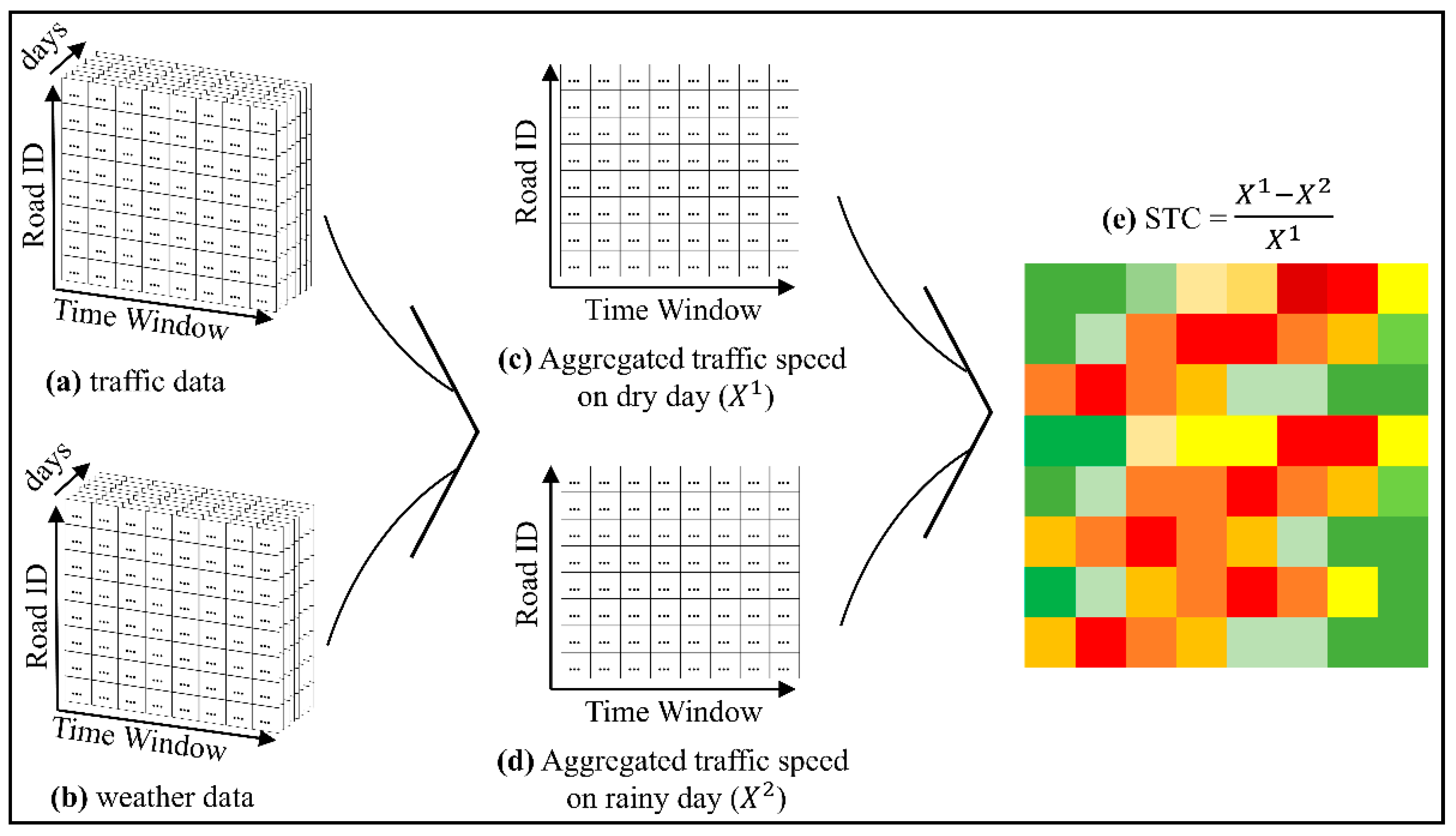
3.1. STC Matrix
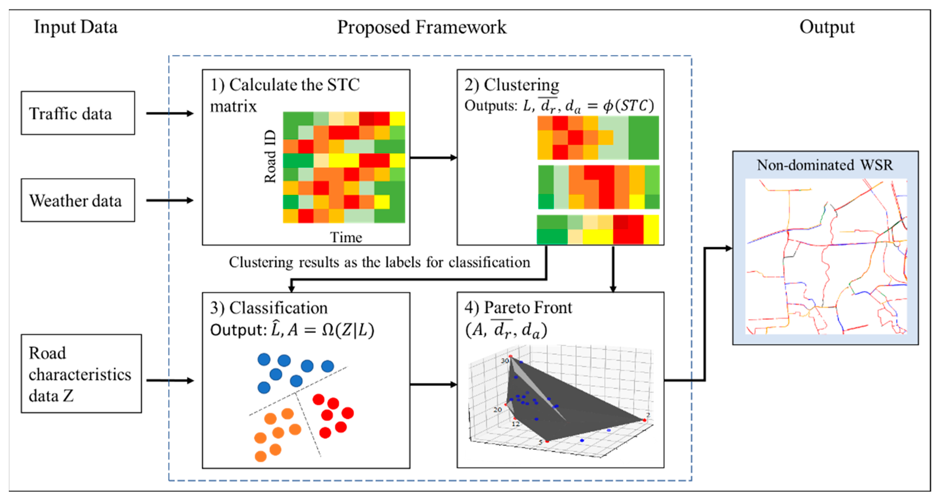
3.2. The Proposed Framework for Analyzing WSR Based on Sequential Clustering and Classification Analysis
- Clustering
- (1)
- Sample k roads without replacement from set X randomly.
- (2)
- Assign the roads to set , and set the initial clusters’ centroid equal to the assigned roads.
- (3)
- Draw a road without replacement from set X randomly ().
- (4)
- Find the nearest set to , , where is equal to 1 if , else 0. also represents the assignment of road to sets .
- (5)
- Update the cluster centroids, .
- (6)
- Repeat steps 3–5 until convergence. Generally, the K-means clustering algorithm aims to minimize .
- Classification
- (1)
- Sample observations from with replacement.
- (2)
- Sample randomly of the independent variables.
- (3)
- Find the split among all possible split’s location for the -th variable, , to classify the given road label and identifies the cut point p′.
- (4)
- Split the data at the node , assign the data to the left descendant of the decision tree if , and to the right descendant if ′, where .
- (5)
- Repeat steps 2–4 until the tree grows maximally.
- Multiobjective Optimization
4. Results
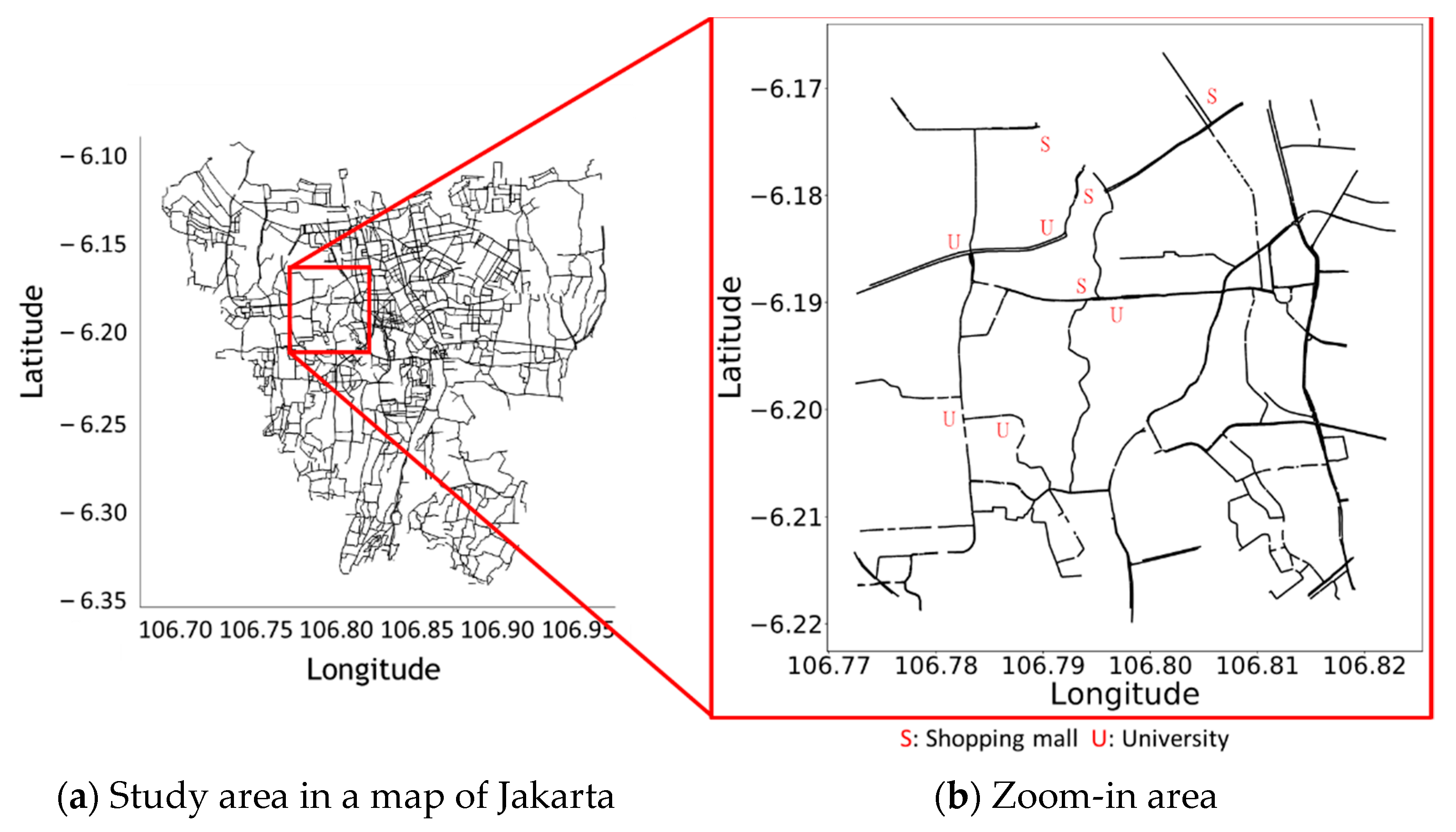
4.1. Dataset
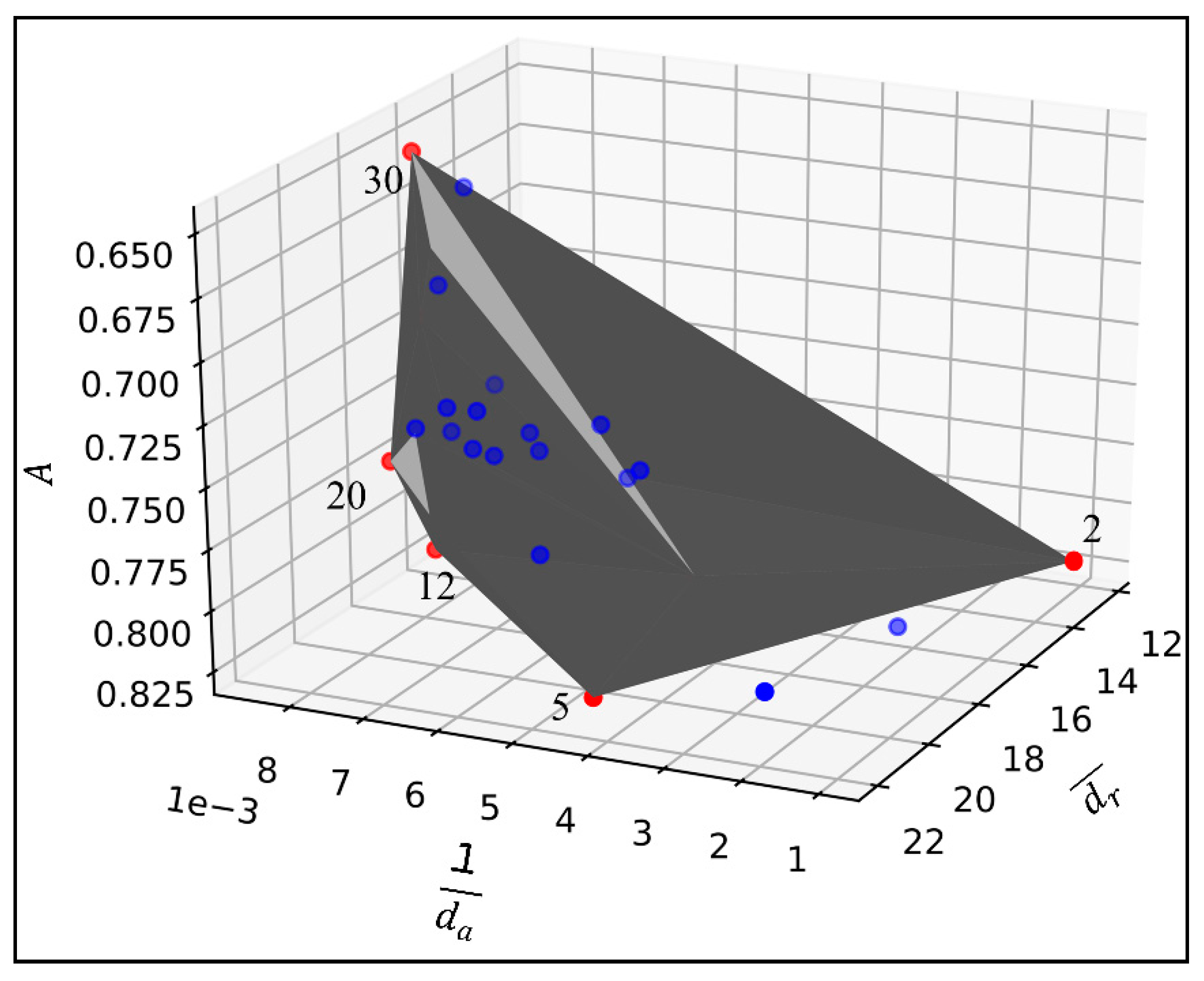
4.2. Selection of K for Clustering
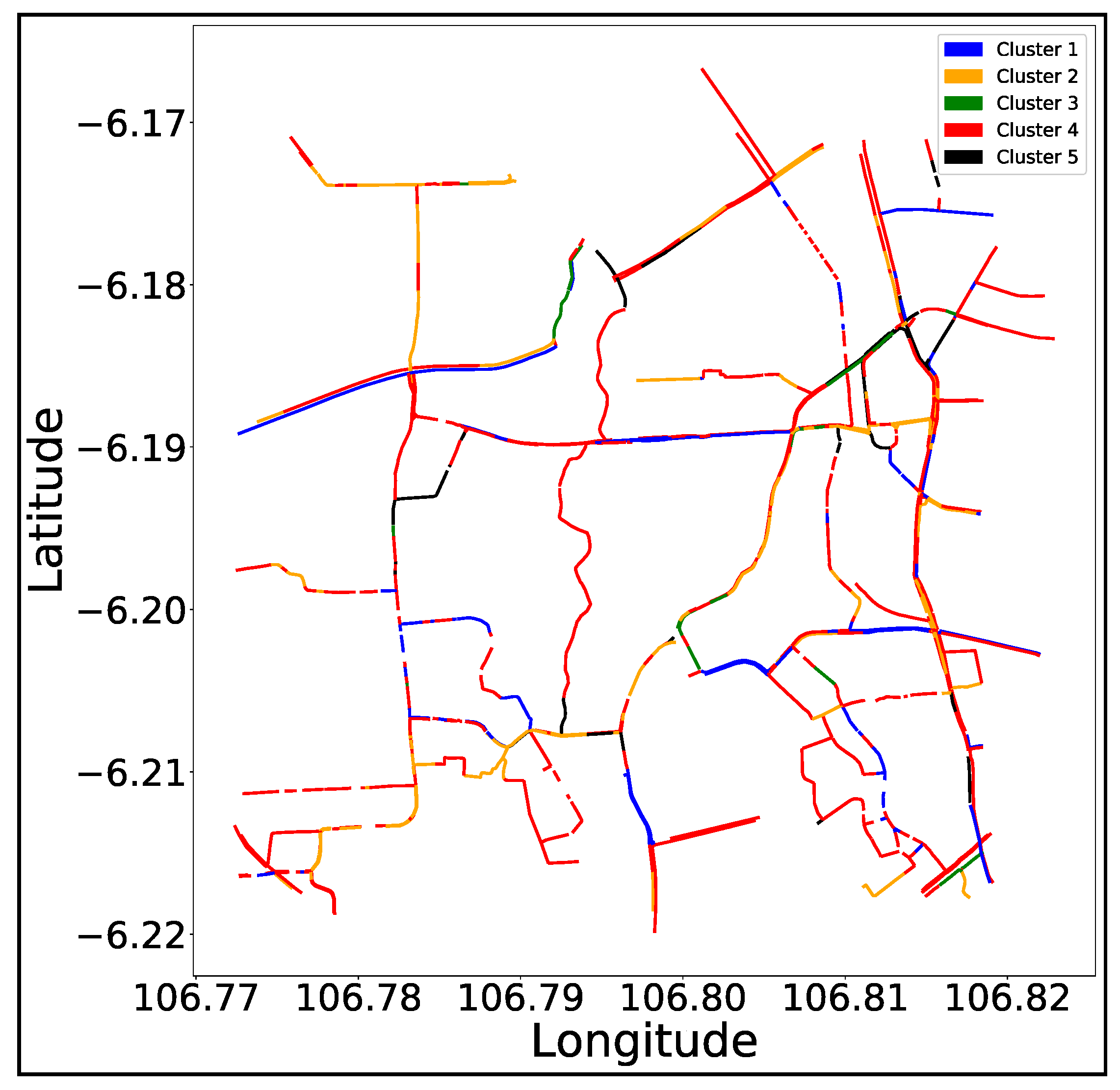
4.3. The WSR Analysis
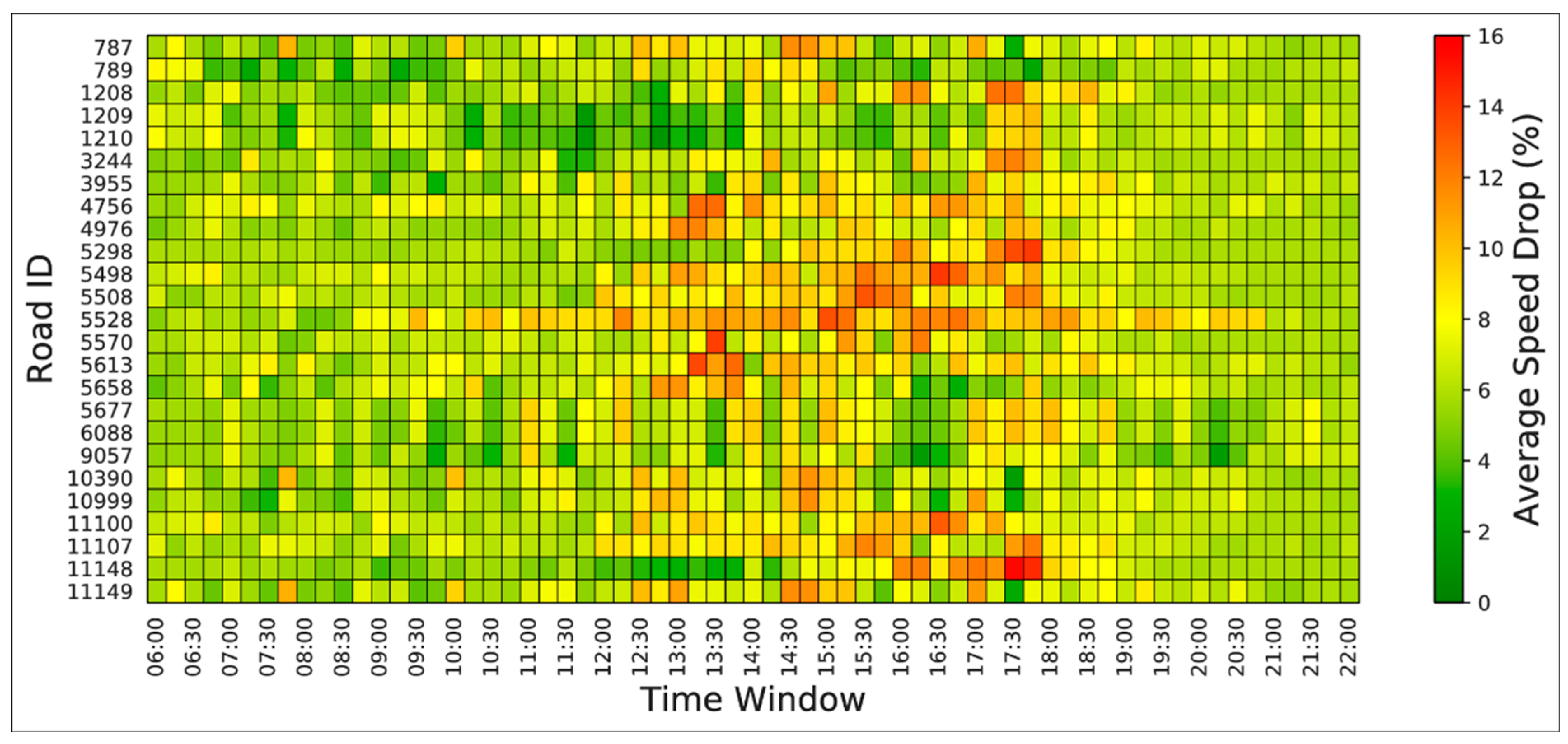
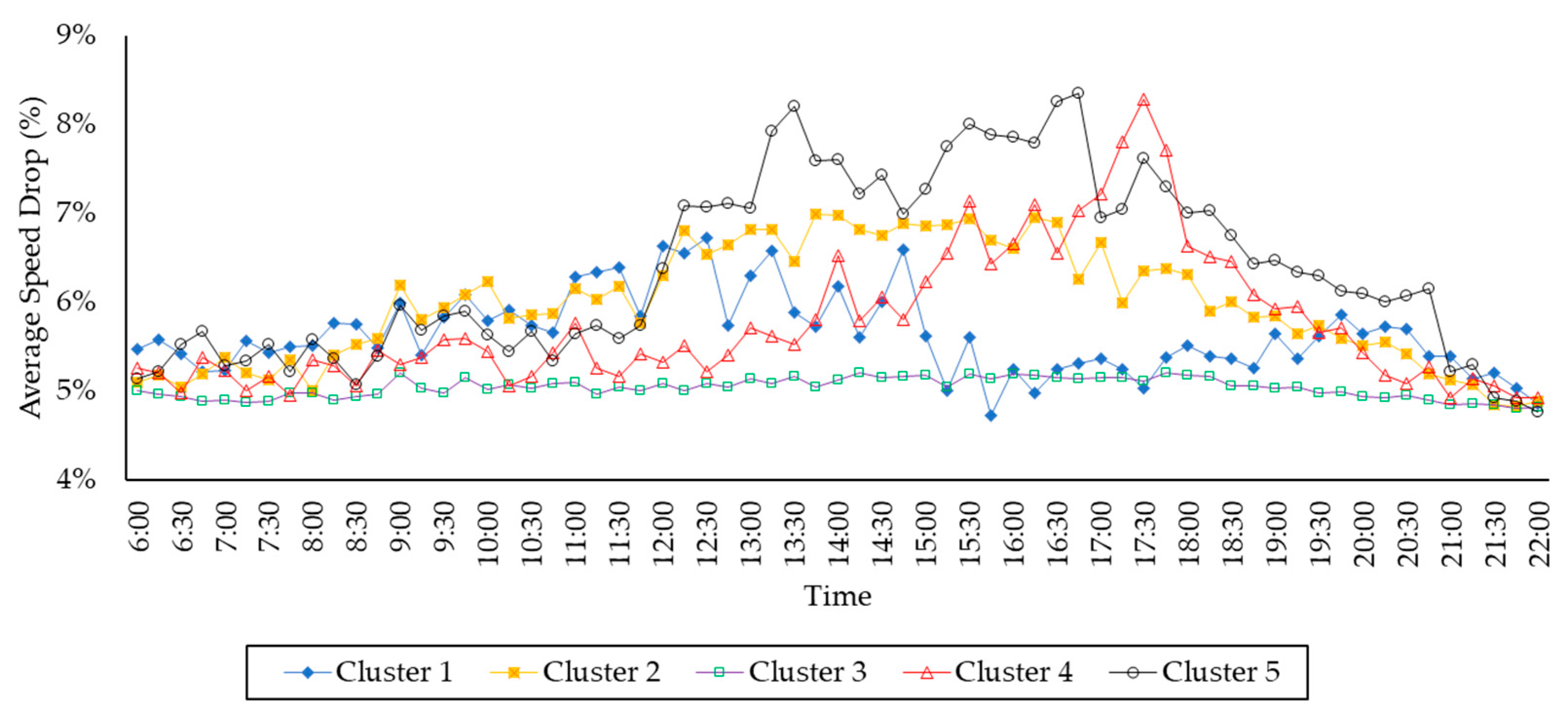
- Speed Drop Pattern
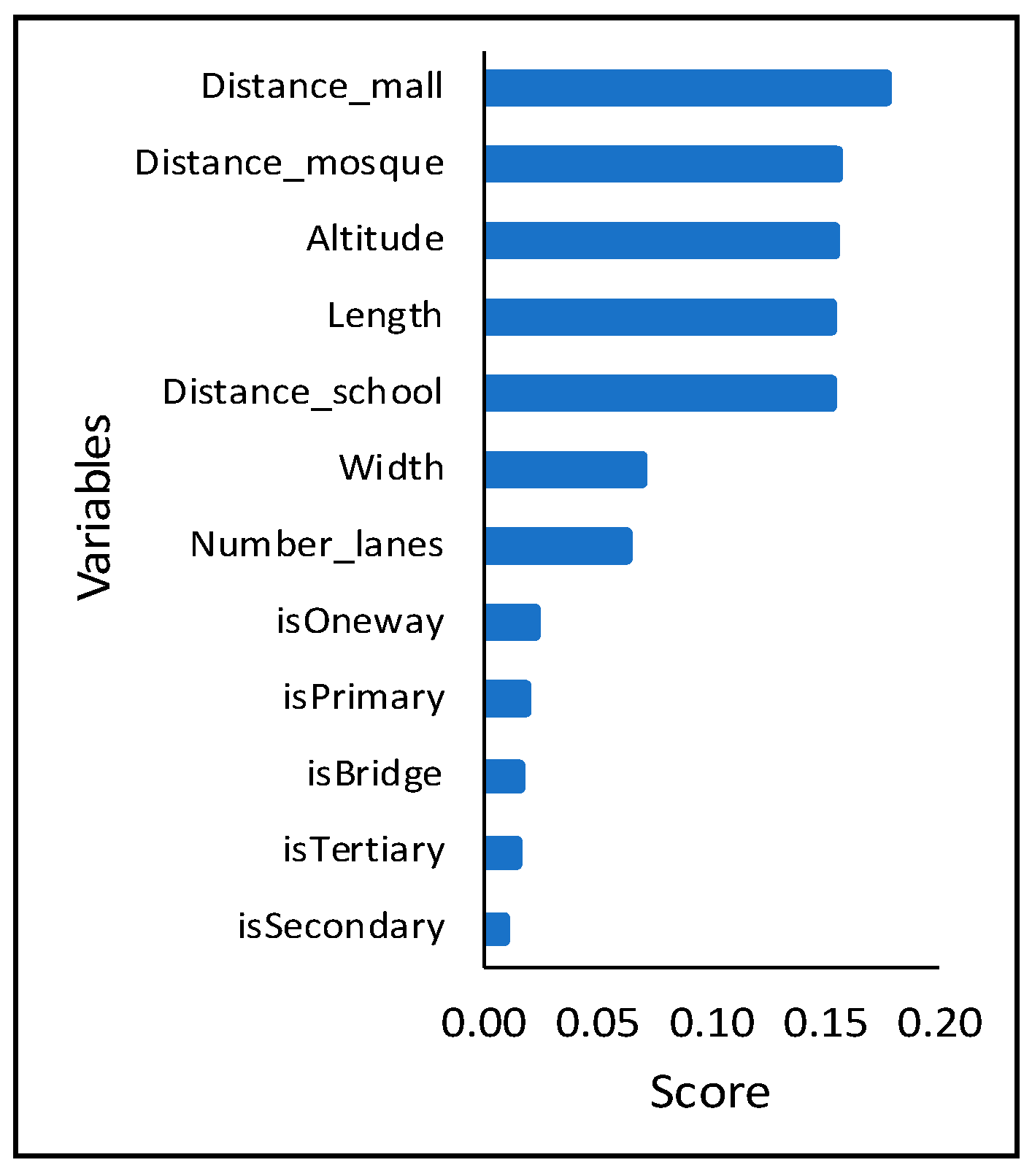
- Road Characteristics Associated with WSR
5. Conclusions
Author Contributions
Funding
Institutional Review Board Statement
Informed Consent Statement
Data Availability Statement
Acknowledgments
Conflicts of Interest
References
- Truitt, A. On the back of a motorbike: Middle-class mobility in Ho Chi Minh City, Vietnam. Am. Ethnol. 2008, 35, 3–19. [Google Scholar] [CrossRef]
- Joewono, T.B.; Tarigan, A.K.M.; Susilo, Y.O. Road-based public transportation in urban areas of Indonesia: What policies do users expect to improve the service quality? Transp. Policy 2016, 49, 114–124. [Google Scholar] [CrossRef]
- Tampubolon, H.; Yang, C.-L.; Chan, A.S.; Sutrisno, H.; Hua, K.-L. Optimized CapsNet for Traffic Jam Speed Prediction Using Mobile Sensor Data under Urban Swarming Transportation. Sensors 2019, 19, 5277. [Google Scholar] [CrossRef] [PubMed] [Green Version]
- Desk, N. Jakarta foots US$5b annual bill for traffic jams: Minister. In The Jakarta Post; PT Bina Media: Tenggara, Jakarta, 2017. [Google Scholar]
- Haider, A.A. Traffic Jam: The Ugly Side of Dhaka’s Development. Last Modified on 13 May 2018. Available online: https://www.thedailystar.net/opinion/society/traffic-jam-the-ugly-side-dhakas-development-1575355 (accessed on 29 March 2021).
- Japan International Cooperation Agency. JICA to Help Philippines Ease Traffic Congestion in Metro Manila; Japan International Cooperation Agency: Tokyo, Japan, 2018; Available online: https://www.jica.go.jp/philippine/english/office/topics/news/180920.html (accessed on 29 March 2021).
- Camacho, F.J.; García, A.; Belda, E. Analysis of Impact of Adverse Weather on Freeway Free-Flow Speed in Spain. Transp. Res. Rec. J. Transp. Res. Board 2010, 2169, 150–159. [Google Scholar] [CrossRef]
- Lam, W.H.K.; Tam, M.L.; Cao, X.; Li, X. Modeling the Effects of Rainfall Intensity on Traffic Speed, Flow, and Density Relationships for Urban Roads. J. Transp. Eng. 2013, 139, 758–770. [Google Scholar] [CrossRef]
- Sathiaraj, D.; Punkasem, T.-O.; Wang, F.; Seedah, D.P.K. Data-driven analysis on the effects of extreme weather elements on traffic volume in Atlanta, GA, USA. Comput. Environ. Urban Syst. 2018, 72, 212–220. [Google Scholar] [CrossRef]
- The Department of Transportation, Taipei City Government. Taipei City ATIS Web. Available online: https://its.taipei.gov.tw/?lang=en (accessed on 26 January 2021).
- Marino, F.; Leccese, F.; Pizzuti, S. Adaptive Street Lighting Predictive Control. Energy Procedia 2017, 111, 790–799. [Google Scholar] [CrossRef]
- Billot, R.; Faouzi, N.-E.E.; Vuyst, F.D. Multilevel Assessment of the Impact of Rain on Drivers’ Behavior: Standardized Methodology and Empirical Analysis. Transp. Res. Rec. J. Transp. Res. Board 2009, 2107, 134–142. [Google Scholar] [CrossRef] [Green Version]
- Hou, T.; Mahmassani, H.S.; Alfelor, R.M.; Kim, J.; Saberi, M. Calibration of Traffic Flow Models Under Adverse Weather and Application in Mesoscopic Network Simulation. Transp. Res. Rec. J. Transp. Res. Board 2013, 2391, 92–104. [Google Scholar] [CrossRef] [Green Version]
- Hooper, E.; Chapman, L.; Quinn, A. The impact of precipitation on speed–flow relationships along a UK motorway corridor. Theor. Appl. Climatol. 2014, 117, 303–316. [Google Scholar] [CrossRef]
- Zhang, W.; Li, R.; Shang, P.; Liu, H. Impact Analysis of Rainfall on Traffic Flow Characteristics in Beijing. Int. J. Intell. Transp. Syst. Res. 2019, 17, 150–160. [Google Scholar] [CrossRef]
- Ji, X.; Shao, C. Modeling and Analyzing Free-Flow Speed of Environment Traffic Flow in Rainstorm Based on Geomagnetic Detector Data. Ekoloji 2019, 28, 4223–4230. [Google Scholar]
- Choo, K.-S.; Kang, D.-H.; Kim, B.-S. Impact Assessment of Urban Flood on Traffic Disruption using Rainfall–Depth–Vehicle Speed Relationship. Water 2020, 12, 926. [Google Scholar] [CrossRef] [Green Version]
- Akbar, A. Berapa Kepadatan Penduduk DKI Jakarta saat ini? Available online: https://statistik.jakarta.go.id/berapa-kepadatan-penduduk-dki-jakarta-saat-ini/ (accessed on 29 March 2021).
- TomTom. Traffic Index 2019. Available online: https://www.tomtom.com/en_gb/traffic-index/ranking/ (accessed on 29 March 2021).
- Nunez, K. Does Your Jogging Speed Feel Right? Available online: https://www.healthline.com/health/average-jogging-speed (accessed on 12 January 2021).
- Yang, C.-L.; Quyen, N.T.P. Data analysis framework of sequential clustering and classification using non-dominated sorting genetic algorithm. Appl. Soft Comput. 2018, 69, 704–718. [Google Scholar] [CrossRef]
- Hartigan, J.A.; Wong, M.A. Algorithm AS 136: A K-Means Clustering Algorithm. J. R. Stat. Society. Ser. C (Appl. Stat.) 1979, 28, 100–108. [Google Scholar] [CrossRef]
- Ho, T.K. Random Decision Forests. In Proceedings of the 3rd International Conference on Document Analysis and Recognition, Montreal, QC, Canada, 14–16 August 1995; pp. 278–282. [Google Scholar]
- Veldhuizen, D.A.V.; Lamont, G.B. Evolutionary computation and convergence to a pareto front. In Proceedings of the Genetic Programming 1998 Conference (GP-98), Madison, WI, USA, 22–25 July 1998; pp. 221–228. [Google Scholar]
- Mitsakis, E.; Stamos, I.; Diakakis, M.; Grau, J.M.S. Impacts of High-Intensity Storms on Urban Transportation: Applying Traffic Flow Control Methodologies for Quantifying the Effects. Int. J. Environ. Sci. Technol. 2014, 11, 2145–2154. [Google Scholar] [CrossRef] [Green Version]
- Stamos, I.; Grau, J.M.S.; Mitsakis, E.; Aifadopoulou, G. Modeling Effects of Precipitation on Vehicle Speed. Transp. Res. Rec. J. Transp. Res. Board 2016, 2551, 100–110. [Google Scholar] [CrossRef]
- Kidando, E.; Kitali, A.E.; Lyimo, S.M.; Sando, T.; Moses, R.; Kwigizile, V.; Chimba, D. Applying Probabilistic Model to Quantify Influence of Rainy Weather on Stochastic and Dynamic Transition of Traffic Conditions. J. Transp. Eng. Part A Syst. 2019, 145, 04019017. [Google Scholar] [CrossRef]
- Yao, Y.; Wu, D.; Hong, Y.; Chen, D.; Liang, Z.; Guan, Q.; Liang, X.; Dai, L. Analyzing the Effects of Rainfall on Urban Traffic-Congestion Bottlenecks. IEEE J. Sel. Top. Appl. Earth Obs. Remote Sens. 2020, 13, 504–512. [Google Scholar] [CrossRef]
- Dunne, S.; Ghosh, B. Weather Adaptive Traffic Prediction Using Neurowavelet Models. IEEE Trans. Intell. Transp. Syst. 2013, 14, 370–379. [Google Scholar] [CrossRef]
- Chen, Y.-Y.; Lv, Y.; Li, Z.; Wang, F.-Y. Long short-term memory model for traffic congestion prediction with online open data. In Proceedings of the 2016 IEEE 19th International Conference on Intelligent Transportation Systems (ITSC), Rio de Janeiro, Brazil, 1–4 November 2016. [Google Scholar]
- Kim, J.; Wang, G. Diagnosis and Prediction of Traffic Congestion on Urban Road Networks Using Bayesian Networks. Transp. Res. Rec. J. Transp. Res. Board 2016, 2595, 108–118. [Google Scholar] [CrossRef] [Green Version]
- Koesdwiady, A.; Soua, R.; Karray, F. Improving Traffic Flow Prediction With Weather Information in Connected Cars: A Deep Learning Approach. IEEE Trans. Veh. Technol. 2016, 65, 9508–9517. [Google Scholar] [CrossRef]
- Lin, L.; Ni, M.; He, Q.; Gao, J.; Sadek, A.W. Modeling the Impacts of Inclement Weather on Freeway Traffic Speed: Exploratory Study with Social Media Data. Transp. Res. Rec. J. Transp. Res. Board 2015, 2482, 82–89. [Google Scholar] [CrossRef] [Green Version]
- Jägerbrand, A.K.; Sjöbergh, J. Effects of weather conditions, light conditions, and road lighting on vehicle speed. SpringerPlus 2016, 5. [Google Scholar] [CrossRef]
- Kurte, K.; Ravulaparthy, S.; Berres, A.; Allen, M.; Sanyal, J. Regional-scale Spatio-Temporal Analysis of Impacts of Weather on Traffic Speed in Chicago using Probe Data. Procedia Comput. Sci. 2019, 155, 551–558. [Google Scholar] [CrossRef]
- Liu, D. Design of Wireless Sensor Intelligent Traffic Control System based on K-means Algorithm. Rev. De La Fac. De Ing. 2017, 32, 354–362. [Google Scholar]
- Pattanaik, V.; Singh, M.; Gupta, P.; Singh, S. Smart real-time traffic congestion estimation and clustering technique for urban vehicular roads. In Proceedings of the 2016 IEEE Region 10 Conference (TENCON), Singapore, 22–25 November 2016; pp. 3420–3423. [Google Scholar]
- Hongsakham, W.; Pattara-atikom, W.; Peachavanish, R. Estimating road traffic congestion from cellular handoff information using cell-based neural networks and K-means clustering. In Proceedings of the 2008 5th International Conference on Electrical Engineering/Electronics, Computer, Telecommunications and Information Technology, Krabi, Thailand, 14–17 May 2008; pp. 13–16. [Google Scholar]
- Breiman, L. Random forests. Mach. Learn. 2001, 45, 5–32. [Google Scholar] [CrossRef] [Green Version]
- Wang, L.; Shi, Q.; Abdel-Aty, M. Predicting Crashes on Expressway Ramps with Real-Time Traffic and Weather Data. Transp. Res. Rec. J. Transp. Res. Board 2015, 2514, 32–38. [Google Scholar] [CrossRef]
- Lee, J.; Nam, B.; Abdel-Aty, M. Effects of Pavement Surface Conditions on Traffic Crash Severity. J. Transp. Eng. 2015, 141. [Google Scholar] [CrossRef]
- OpenStreetMap Data Working Group. Available online: https://planet.osm.org (accessed on 29 March 2021).
- Li, T.; Zhang, C.; Zhu, S. Empirical Studies on Multi-label Classification. In Proceedings of the 18th IEEE International Conference on Tools with Artificial Intelligence (ICTAI’06), Arlington, VA, USA, 13–15 November 2006. [Google Scholar]
- World Weather Online. Available online: https://www.worldweatheronline.com/developer/api/local-city-town-weather-api.aspx (accessed on 29 March 2021).
- Merry, K.; Bettinger, P. Smartphone GPS accuracy study in an urban environment. PLoS ONE 2019, 14, e0219890. [Google Scholar] [CrossRef] [PubMed] [Green Version]


| Longitude | Latitude | Speed (km/h) | Level | Time |
|---|---|---|---|---|
| 106.782318 | −6.198835 | 2.91 | 3 | 17 November 2017 00:18:56 |
| 106.899734 | −6.218775 | 1.32 | 4 | 16 November 2017 23:34:48 |
| 106.782875 | −6.333290 | 3.44 | 3 | 17 November 2017 00:04:58 |
| 106.825172 | −6.187048 | 2.31 | 3 | 17 November 2017 00:02:35 |
| 106.738625 | −6.126846 | 3.51 | 3 | 17 November 2017 00:11:52 |
| Date | Month | Time | Weather | Temperature | Precipitation | Year |
|---|---|---|---|---|---|---|
| Tue 01 | Aug | 0:00 | Patchy rain possible | 29 | 0 | 2017 |
| Tue 01 | Aug | 3:00 | Partly cloudy | 30 | 0 | 2017 |
| Tue 01 | Aug | 6:00 | Cloudy | 33 | 0 | 2017 |
| Tue 01 | Aug | 12:00 | Sunny | 38 | 0 | 2017 |
| Tue 01 | Aug | 18:00 | Clear | 35 | 0 | 2017 |
| Name | Description |
|---|---|
| isBridge | 1—If the road is a bridge, 0—otherwise |
| isOneway | 1—If the road applies the one-way policy, 0—otherwise |
| isPrimary | 1—If the road is the main road, 0—otherwise |
| isSecondary | 1—If the road is the secondary road, 0—otherwise |
| isTertiary | 1—If the road is the tertiary road, 0—otherwise |
| Length | Length of the road in meter unit |
| Width | Width of the road in meter unit |
| Number_lanes | Number of lanes |
| Type_road | Three types: primary, secondary, tertiary |
| Altitude | The road’s altitude (meter) above the sea |
| Distance_school | Distance (meter) to the nearest school to the road segment |
| Distance_mosque | Distance (meter) to the nearest mosque to the road segment |
| Distance_mall | Distance (meter) to the nearest mall to the road segment |
| 2 | 12.267 | 0.001 | 0.822 |
| 5 | 22.000 | 0.004 | 0.817 |
| 12 | 20.831 | 0.006 | 0.770 |
| 20 | 19.454 | 0.007 | 0.740 |
| 30 | 16.863 | 0.008 | 0.652 |
| Variables | Cluster 1 | Cluster 2 | Cluster 3 | Cluster 4 | Cluster 5 |
|---|---|---|---|---|---|
| Distance_mall | 975.1 | 1256.5 | 1069.8 | 966.5 | 650.8 |
| Distance_mosque | 149.3 | 178.7 | 146.2 | 127.9 | 192.7 |
| Length | 150.2 | 98.7 | 91.1 | 151.7 | 135.2 |
| Width | 6.26 | 6.68 | 6.23 | 7.00 | 8.33 |
| Number_lanes | 1.87 | 2.57 | 2.01 | 2.10 | 2.48 |
| Altitude | 10.29 | 10.32 | 10.69 | 8.68 | 10.02 |
| Distance_school | 232.3 | 203.3 | 192.3 | 174.1 | 240.4 |
Publisher’s Note: MDPI stays neutral with regard to jurisdictional claims in published maps and institutional affiliations. |
© 2021 by the authors. Licensee MDPI, Basel, Switzerland. This article is an open access article distributed under the terms and conditions of the Creative Commons Attribution (CC BY) license (https://creativecommons.org/licenses/by/4.0/).
Share and Cite
Yang, C.-L.; Sutrisno, H.; Chan, A.S.; Tampubolon, H.; Wibowo, B.S. Identification and Analysis of Weather-Sensitive Roads Based on Smartphone Sensor Data: A Case Study in Jakarta. Sensors 2021, 21, 2405. https://0-doi-org.brum.beds.ac.uk/10.3390/s21072405
Yang C-L, Sutrisno H, Chan AS, Tampubolon H, Wibowo BS. Identification and Analysis of Weather-Sensitive Roads Based on Smartphone Sensor Data: A Case Study in Jakarta. Sensors. 2021; 21(7):2405. https://0-doi-org.brum.beds.ac.uk/10.3390/s21072405
Chicago/Turabian StyleYang, Chao-Lung, Hendri Sutrisno, Arnold Samuel Chan, Hendrik Tampubolon, and Budhi Sholeh Wibowo. 2021. "Identification and Analysis of Weather-Sensitive Roads Based on Smartphone Sensor Data: A Case Study in Jakarta" Sensors 21, no. 7: 2405. https://0-doi-org.brum.beds.ac.uk/10.3390/s21072405