
Clusters of Spin Valve Sensors in 3D Magnetic Field of a Label
by
 ,
,
Georgy V. Babaytsev
, 
Nikolay G. Chechenin
*,
Irina O. Dzhun
,
Mikhail G. Kozin
,
Alexey V. Makunin
and
Irina L. Romashkina
Skobeltsyn Institute of Nuclear Physics, Lomonosov Moscow State University, Leninskie Gory 1/2, 119991 Moscow, Russia
*
Author to whom correspondence should be addressed.
Sensors 2021, 21(11), 3595; https://0-doi-org.brum.beds.ac.uk/10.3390/s21113595
Submission received: 12 April 2021
/
Revised: 11 May 2021
/
Accepted: 18 May 2021
/
Published: 21 May 2021
(This article belongs to the Special Issue Design and Applications of Magnetic Sensors)
Abstract
:Magnetic field sensors based on the giant magnetoresistance (GMR) effect have a number of practical current and future applications. We report on a modeling of the magnetoresistive response of moving spin-valve (SV) GMR sensors combined in certain cluster networks to an inhomogeneous magnetic field of a label. We predicted a large variety of sensor responses dependent on the number of sensors in the cluster, their types of interconnections, the orientation of the cluster, and the trajectory of sensor motion relative to the label. The model included a specific shape of the label, producing an inhomogeneous magnetic field. The results can be used for the optimal design of positioning devices.
1. Introduction
Magnetic field sensors based on various physical effects play an important role in modern science, industry, and everyday life. A number of reviews have been published on applications of sensors in different spheres. A review of applications of modern, highly sensitive magnetometers can be found in Grosz and Haji-Sheikh [1]. A comprehensive review focused primarily on biological and medical applications of different types of magnetic field sensors is given in Murzin et al. [2]. Among the basic principles of sensor functioning, magnetoresistance (MR) has the widest scope of development and applications. A roadmap of this type of sensor was recently published [3]. Sensors employing the anisotropic, giant, and tunnel magnetoresistance effects are becoming more and more competitive because they can offer a variety of attractive properties suited for specific uses. MR sensors offer high sensitivity sought for biomedical applications [2,3,4,5,6,7]; high mechanical flexibility, small size, and robustness for wearable and portable devices [8,9,10,11]; low power consumption and small physical size, for position sensing [12,13,14]; low cost and mass production for large-scale, non-destructive evaluation and monitoring systems [15,16,17,18]; high accuracy and stability for navigation and transportation systems [19,20,21,22]; and high radiation hardness for space applications [13,14,16,21,22,23].
Spin-valve (SV) sensors are a type of magnetic field sensor based on the giant magnetoresistance (GMR) effect, discovered by two research groups led by Nobel Prize Laureates for Physics in 2007 Albert Fert [24] and Peter Grünberg [25]. Different aspects of the nature of the GMR effect and applications of the effect in magnetoresistive sensors are presented in [26]. SV sensors are a specific type of GMR sensor. The output signal of a SV sensor depends on the applied magnetic field via the angle ϕ between magnetizations of the free and pinned ferromagnetic layers of SV structure by (1-cosϕ) law [27]. This law follows from the Stoner-Wohlfarth model of coherent rotation of free layer magnetization [28]. Despite the fact that this model oversimplifies the real picture, it captures the main features of the phenomenon and allows the calculation of GMR as a function of an external magnetic field RGMR(H).
From the experimental side, the angular variation of the GMR effect was found to be very close to the relation RGMR(ϕ) = R0GMR (1 − cosϕ)/2 in the current-in-plane (CIP) geometry for various systems, where R0GMR is the amplitude of the GMR effect [27,29].
Usually, single sensing elements are combined in groups or clusters, the most familiar being a Wheatstone bridge (WB) with one to four active arms in the bridge. The inactive elements are either deactivated by magnetic shielding, or made from nonmagnetic material with close electric resistance.
In the present work, we consider linear movement of a macroscopic ((sub)-millimeter range) sensor in the form of the Wheatstone bridge with one or two point-size sensing elements in the inhomogeneous field of a magnetic label. The magnetic label has macroscopic (millimeter range) dimensions and the form of a cuboid (parallelepiped with square base), cylinder, or other shape that allows calculation of the components of a magnetic field in close vicinity to the label, where it differs from a dipolar field. We calculate the signals of the unbalanced bridge for parallel and perpendicular orientations of sensing element magnetization relative to the direction of linear movement of the bridge parallel to the y-axis of the Cartesian coordinate system with magnetic label in the origin. All sensing elements are deposited in the same plane on the surface of a substrate. We investigate the dependence of the signal on the size of the bridge and on the nearest approaching distance between the bridge center and the label along the trajectory, referred to as the impact parameter.
Despite the fact that the Wheatstone bridge configuration is a common subject in the literature [30], to the best of our knowledge, our study is the first to consider in detail the position sensing of a magnetic object using WB. The present results can be used for positioning magnetic objects in 3D space, and for label monitoring with a network of bridge clusters.
2. Materials and Methods
2.1. Simulated Sensors and Magnetic Label
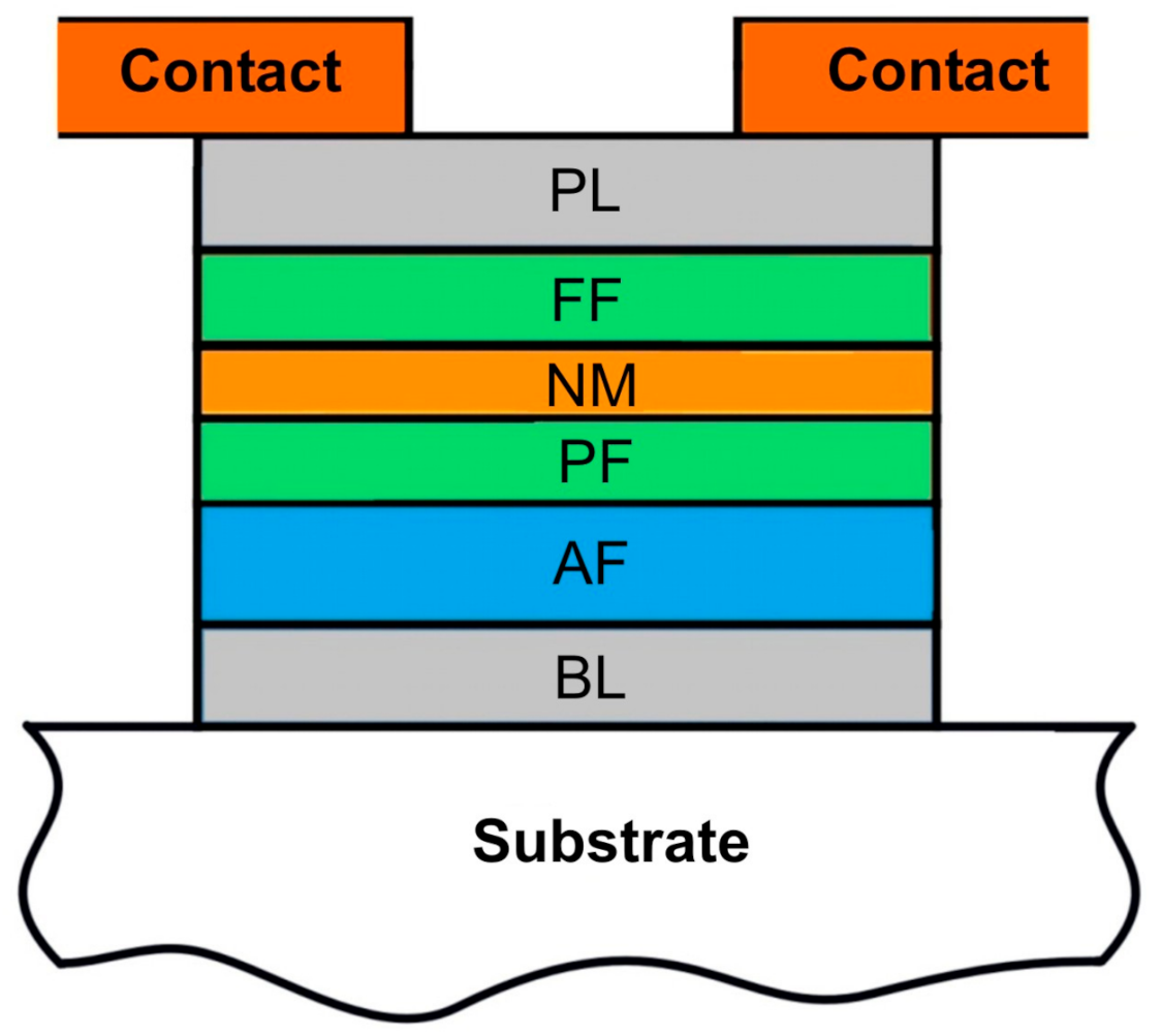
The simulated system consists of a magnetic label and a cluster of SV sensors. In our calculations, we assume the magnetic label is in the form of a cuboid with dimensions of 2 × 2 × 3 mm3 with the remanence Br = 0.4 T, which corresponded to the label parameters in our experiments. The simulated clusters of SV sensors are 4 SV elements configured into a rectangular 4-arm Wheatstone bridge. The SV elements are multilayer structures typically deposited in CIP geometry. A schematic representation of the layers of the SV structure is shown in Figure 1. The layers FF/NM/PF/AF are the most important part of the SV structure, where FF is a free ferromagnetic layer; NM, a non-magnetic layer; PF, a pinned ferromagnetic layer; and AF, an antiferromagnetic layer. It is assumed in the calculations that PF has a strongly pinned orientation of magnetic moment, making PF not sensitive to the external magnetic field. In contrast, the FF layer is made of a soft material with magnetic moment that rotates under the influence of an external magnetic field. The most important magnetic parameters of the FF used in calculation are the saturation magnetization Ms = 100 kA/m and uniaxial anisotropy coefficient Ku = 200 J/m3, corresponding to Permalloy, used in our experiments [31]. The bridge is normally deposited in a single deposition run; therefore, all 4 SV elements were identical, providing the balance in the output signal in the absence of the magnetic field. In addition, 2 or 3 SV elements were shielded so that they were insensitive to the magnetic field, leaving 1 or 2 sensitive SV elements in the bridge.
2.2. Simulation Model
A permanent magnet label creates an inhomogeneous 3D magnetic field. The method of calculating the 3D components of the magnetic field of the label, H(R), was reported earlier [32]. A similar method was used in our previous papers [33,34] to calculate the fields of permanent magnets of several forms (parallelepiped, cylinder, etc.). We chose the Cartesian coordinate system connected with the label placed at the origin and with magnetic moment oriented along the z-axis. Instead of translation of the label, we consider the motion of the sensor along a straight-line trajectory in the yz-plane at a distance x0 from the origin and z0 from the xy plane. We follow the variation of the sensor signal during the motion along the trajectory, i.e., we study the variation of the signal depending on the sensor location relative to the label and on the relative mutual orientation of the sensor and the magnetic label. The results for orientations of 6 single sensors were given in Babaitsev et al. [33,34] are used here for clusters of SV sensors.
The single sensor is supposed to be a point-like object characterized by direction of uniaxial anisotropy in the free ferromagnetic (FF) layer and unidirectional anisotropy in the ferromagnetic pinned (FP) layer, defined by the direction of the magnetic field during the deposition of the layers. The orientation of the structure is characterized by the normal n to the plane of the multilayer structure of the sensor. The vector M is the magnetic moment of the FF layer; Ms is the value in saturation.
Here we assume that the Stoner-Wohlfarth (SW) model [28,35], which often is used to describe the processes occurring in SV, is also valid for the magnetic film. The model allows us to evaluate the reorientation of the magnetization of the anisotropic particle under the influence of an applied field. Applying the magnetic field in a direction different from the direction of the easy axis (EA), one can initiate a coherent rotation of the magnetic moment M in the FF layer of the SV. Further on, the model assumes that the rotation and equilibrium state of magnetization are achieved instantly. An in-depth consideration of signal features of a single SV sensor moving in a magnetic field of a label can be found in Babaitsev et al. [33,34]. In this paper, we study the signal of a cluster of sensors instead of a single SV sensor.
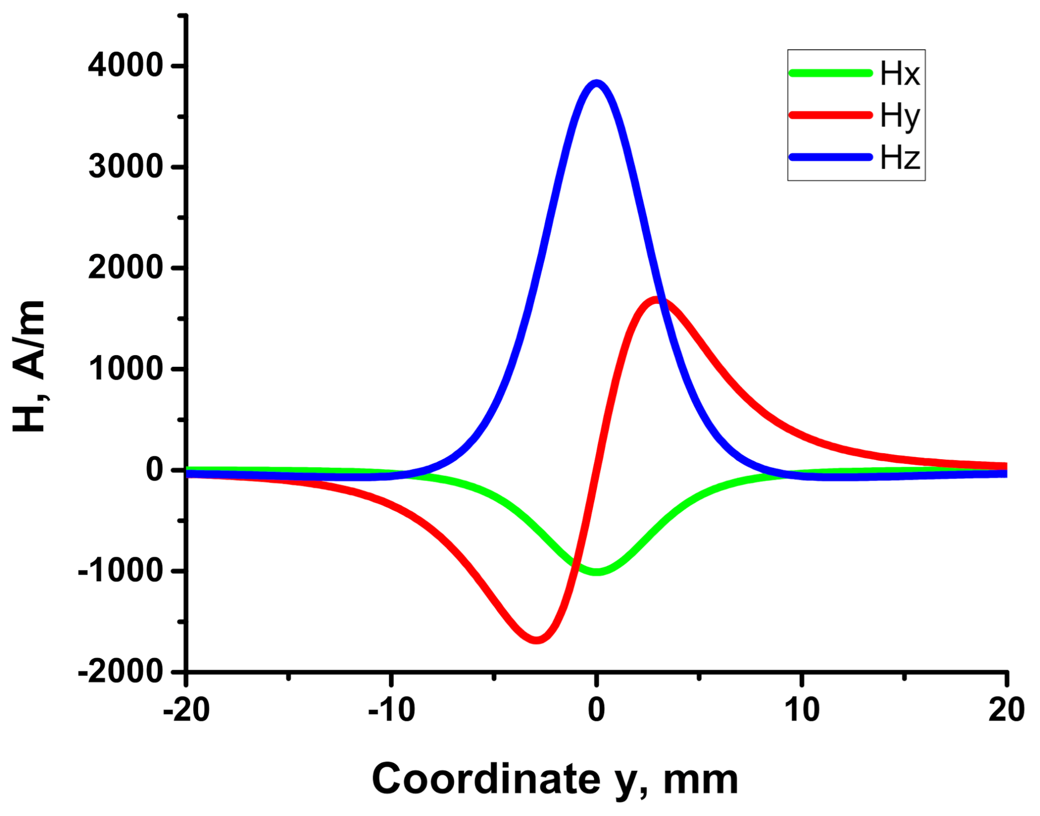
The variation of magnetic field components along the y-direction for a cuboid label is illustrated in Figure 2. There are constant-sign dependences for 2 components of the magnetic field, Hx and Hz, and an alternating-sign for another one, Hy. Similar calculations can be made for magnetic labels in the form of a cylinder or ball.
2.3. Interaction of the Magnetic Label and the Cluster of SV Sensors
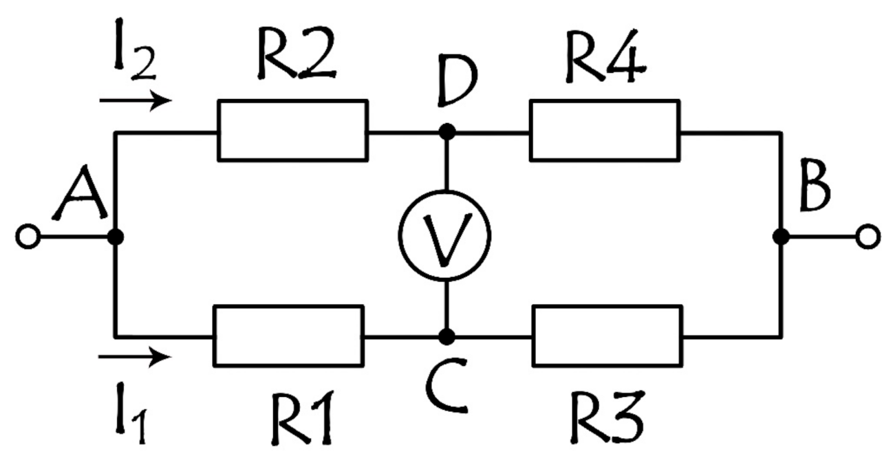
The simplest cluster is the Wheatstone bridge (Figure 3). The principle of operation of the bridge is based on the equalization of potentials of the middle terminals of 2 resistor branches connected in parallel, each of which has 2 resistors.
When powered by voltage, the bridge provides a differential output UDC as a function of resistance change
where UAB is a bias voltage, and R1–R4 are resistances in the arms of the bridge.
In our calculations the bias voltage of the bridge is 10 V, and the resistances of SV RP and RAP are equal to 20 and 22 Ohm (RP and RAP—the resistances at parallel and antiparallel magnetization of free and pinned layers, respectively).
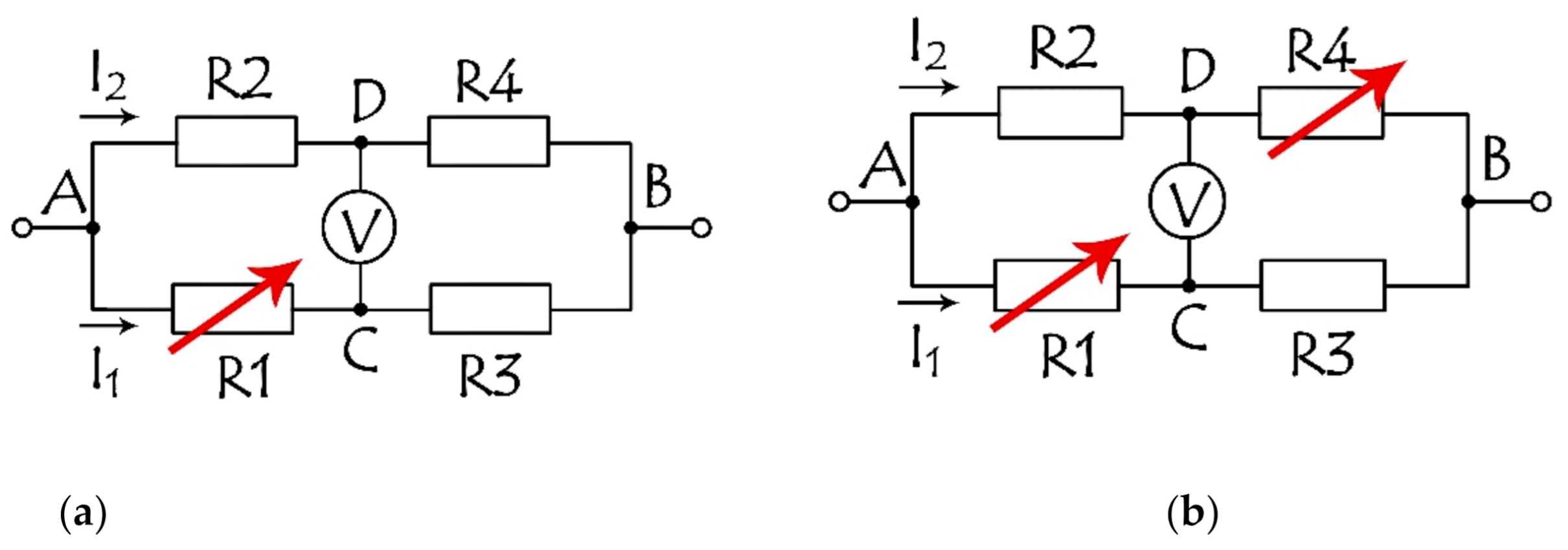
Without a magnetic field, the SV bridge is balanced, and the signal from the bridge is absent. With a magnetic field applied, the signal appears and is recorded by the voltage change. The arms of the bridge are made of identical SV structures to exclude a misbalance in the bridge in a no-field environment and the necessity of adjusting the resistors and construct additional microcircuits for balancing the bridge. The identity can be easily achieved by the SV layer deposition in 1 cycle. Three or two arms can be shielded, making the bridge with one R1 = R + ΔR (Figure 4a), or with two R1 = R + ΔR1, R4 = R + ΔR4 (Figure 4b) sensitive elements in diagonal position. The output voltage as a function of the resistance of 1 or 2 sensitive elements in Figure 4 can be expressed, respectively, as Equation (2) or Equation (3).
3. Results and Discussion
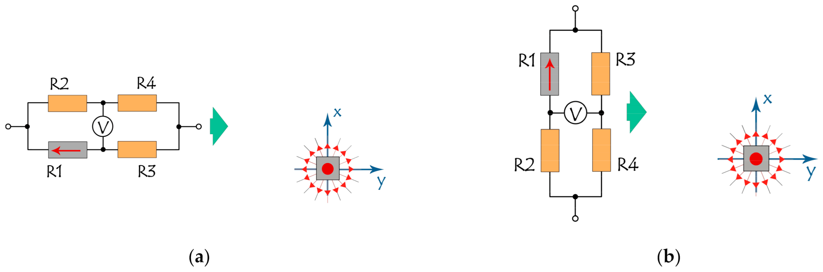
Let us consider first a simplest cluster configuration with one sensitive SV element and the other three of four identical elements shielded, as shown in Figure 5 for two identical sensors with two different orientations with respect to the label. The plane of both sensors is parallel to the XY plane, but the directions of magnetization of the sensitive SV elements are parallel (Figure 5a) or perpendicular (Figure 5b) to the line of movement of the bridge, and both are perpendicular to the magnetic moment of the label.
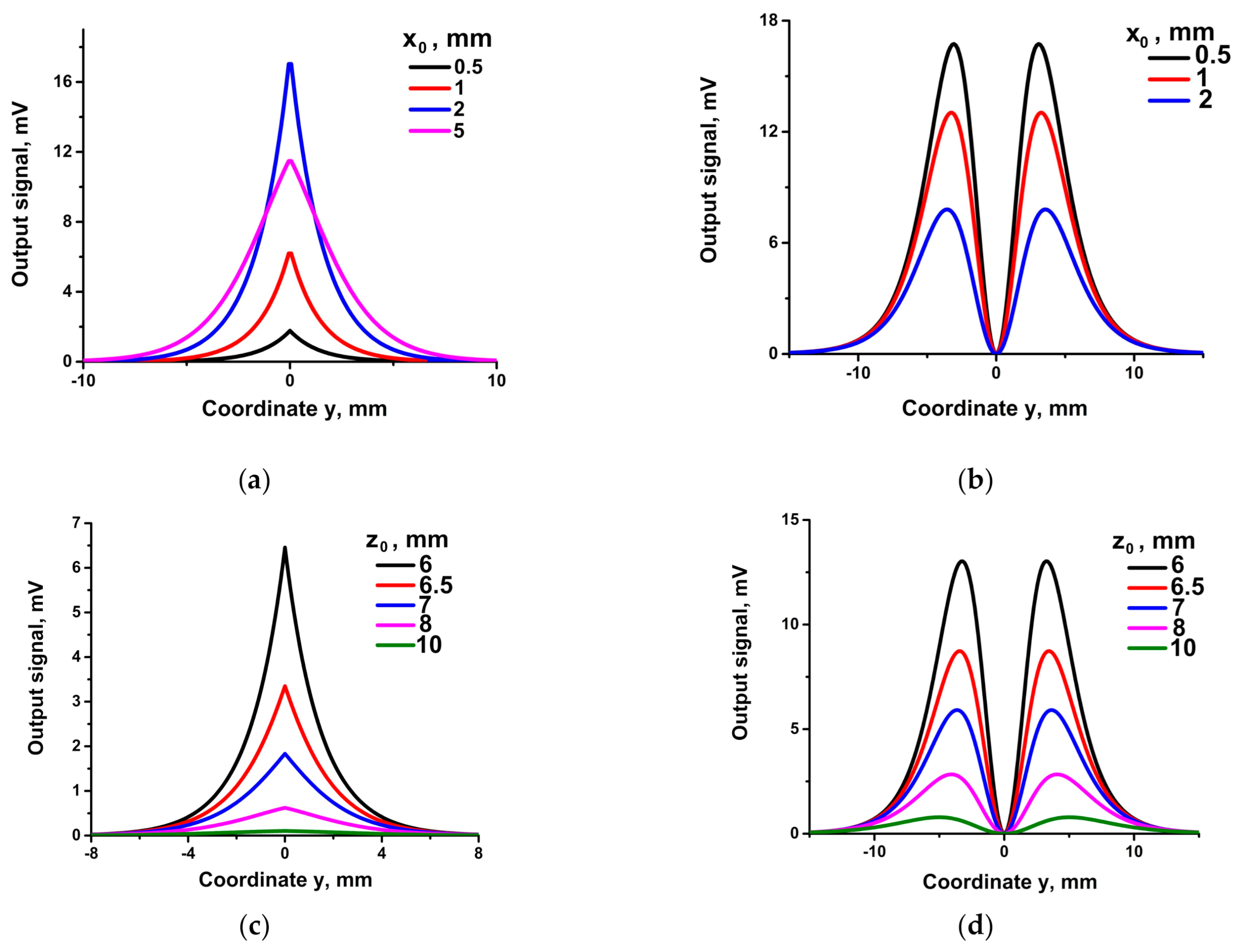
Representative results of numerical calculation of the response of such bridges are shown in Figure 6 (a,b—for different x0-coordinates and c,d—for different z0-coordinates of the R1 element).
The shape of the curves in Figure 6a,c (left panel) is a single peak, while in Figure 6b,d (right panel) the curves have two peaks. In addition, one can note that the output peak value varies in Figure 6a non-monotonously when the parameter x0 increases At first, the peak value increases (curves x0 = 0.5; 1; 2 mm), then decreases (curve x0 = 5 mm) at the same time that the width of curve x0 = 5 mm increases. The non-monotony may look somewhat surprising; the increase of x0 from 0.5 mm to 2 mm, and, hence, the distance from the label magnetic field decreases and should lead at first sight to a smaller rotation of M and smaller signal in R1.
The observed features can be interpreted based on consideration of the output signal of a single SV sensor in the field of a magnetic label reported previously. In particular, the case in Figure 4a corresponds to case 2.1 in Babaitsev et al. [33], when the magnetic moment of the R1 sensor has components M = {Ms, 0, 0} in the initial state. Non-monotony is due to two factors, besides the distance between the sensor and the label. (1) Due to a demagnetizing field vector, M can rotate within the plane of the sensor, i.e., in the xy plane in the case of Figure 5a, so during the movement in y-direction, M will have an in-plane component Mxy with Mz = 0. (2) Only a perpendicular to M component of the magnetic field, except Hz, can cause the tilt of M. Variation of the Hxy (x0, y, z0) components of the 3D field of the magnetic label makes the observed feature of the output signal of the SV sensor a reflection of variation of the tilt angle ϕ = arctg (Mx/My).
Due to the initial orientation of M in Figure 5a, parallel to the y-axis, My = Ms, the dominating rotation action is due to the y-component of non- monotony H. It is important to note that Hy keeps the sign on the trajectories 1–5 in Figure 6a,c, slowly increasing and decreasing when crossing the space plane {x, 0, z}. Therefore, the output signal is of a single-peak shape.
In contrast, the dominating rotational effect on Mx = Ms for the case of Figure 5b is due to the component Hy of the 3D label magnetic field. In this case, the Hy component changes sign when crossing the space plane {x, 0, z}, inducing the double-peak shapes of the curves of y-scan with trajectories {x = x0 = 0.5; 1; 2 mm, y = var; z = z0 = 6 mm} in Figure 6b and {x = x0 = 1 mm, y = var, z0 = z = 6; 6.5; 7; 8; 10 mm} in Figure 6d.
The bridge signal depends only on the R1 coordinate and does not depend on R2–R4 coordinates (i.e., it does not depend on the bridge size). If, instead of R1, we make another sensing arm of the bridge, then the signal polarity for R4, as the sensing element, will be the same as for R1 and of opposite polarity for R2 or R3.
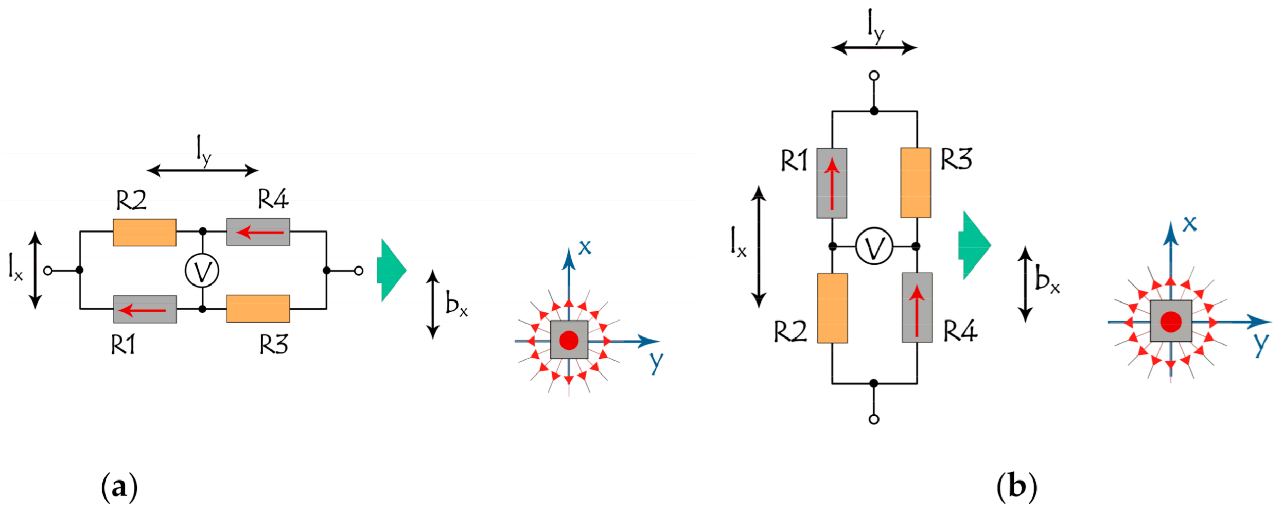
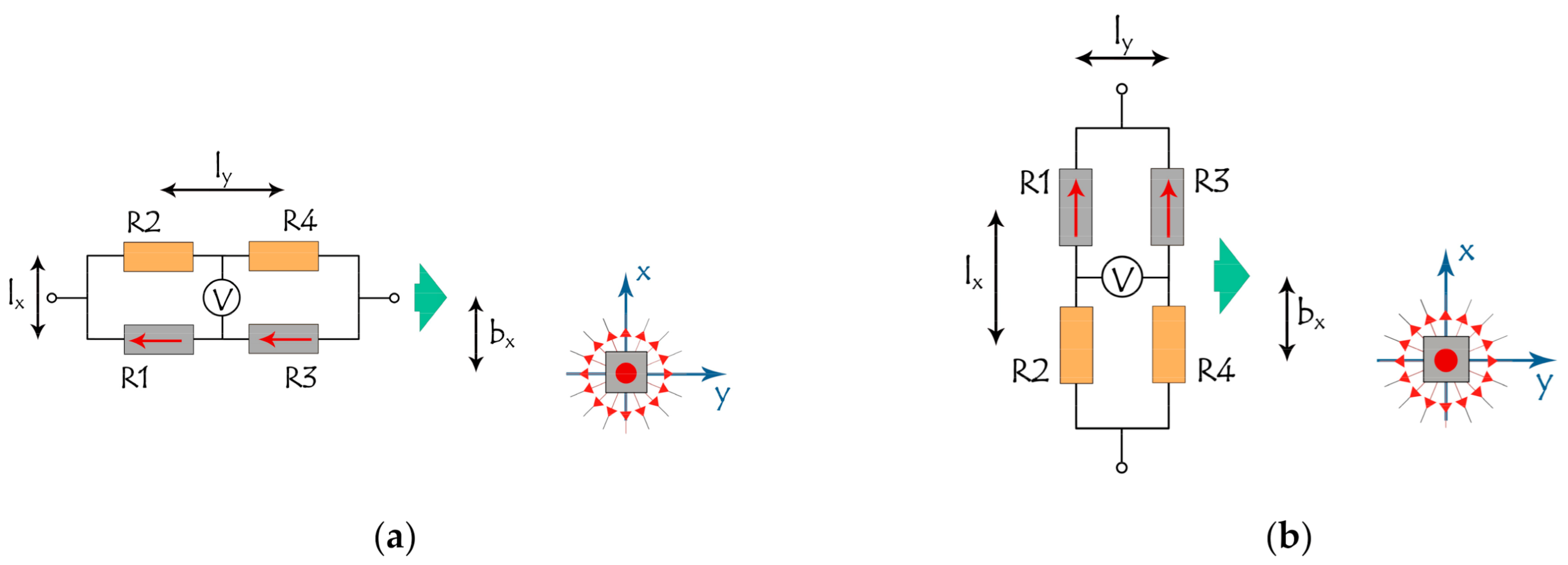
Configurations for a bridge with two sensing elements R1 and R4 are shown in Figure 7. In this case, the dimensions of the SV sensor and locations of the sensing elements within it are important. In Figure 7 the size of the sensor is characterized by distances between sensor elements along the x and y axes, lx and ly. It is also convenient to introduce the parameter bx and bz (the latter is not shown), which, in analogy with the tradition in the field of atomic scattering, are called impact parameters in the x and z directions and are determined as the nearest approach distances between the center of the bridge and the label. These parameters play a role as coordinates of trajectories x0 and z0 in the bridge with a single sensitive element, considered above. Magnetic moments in the sensitive elements in the initial state are aligned in parallel, which is a normal practice in layer deposition and post-deposition treatment.
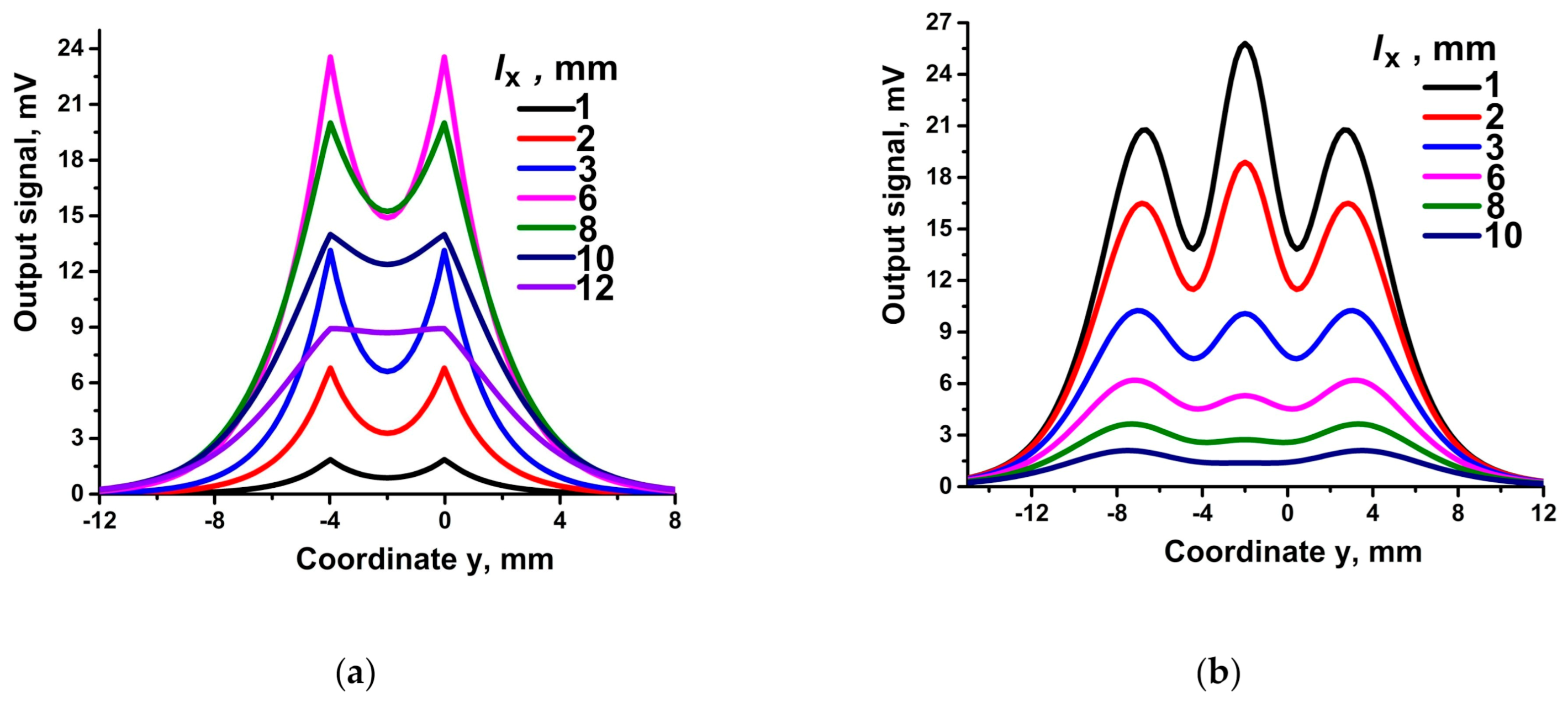
The results of numerical study of the response of such bridges with two orientations relative to the label and the direction of movement are shown in Figure 8, Figure 9 and Figure 10. The left panel in Figure 8, Figure 9 and Figure 10 corresponds to the y-orientation of the magnetic moments My = Ms in the sensitive elements, Figure 7a, while the right panel relates to the x-orientation, Mx = Ms, Figure 7b.
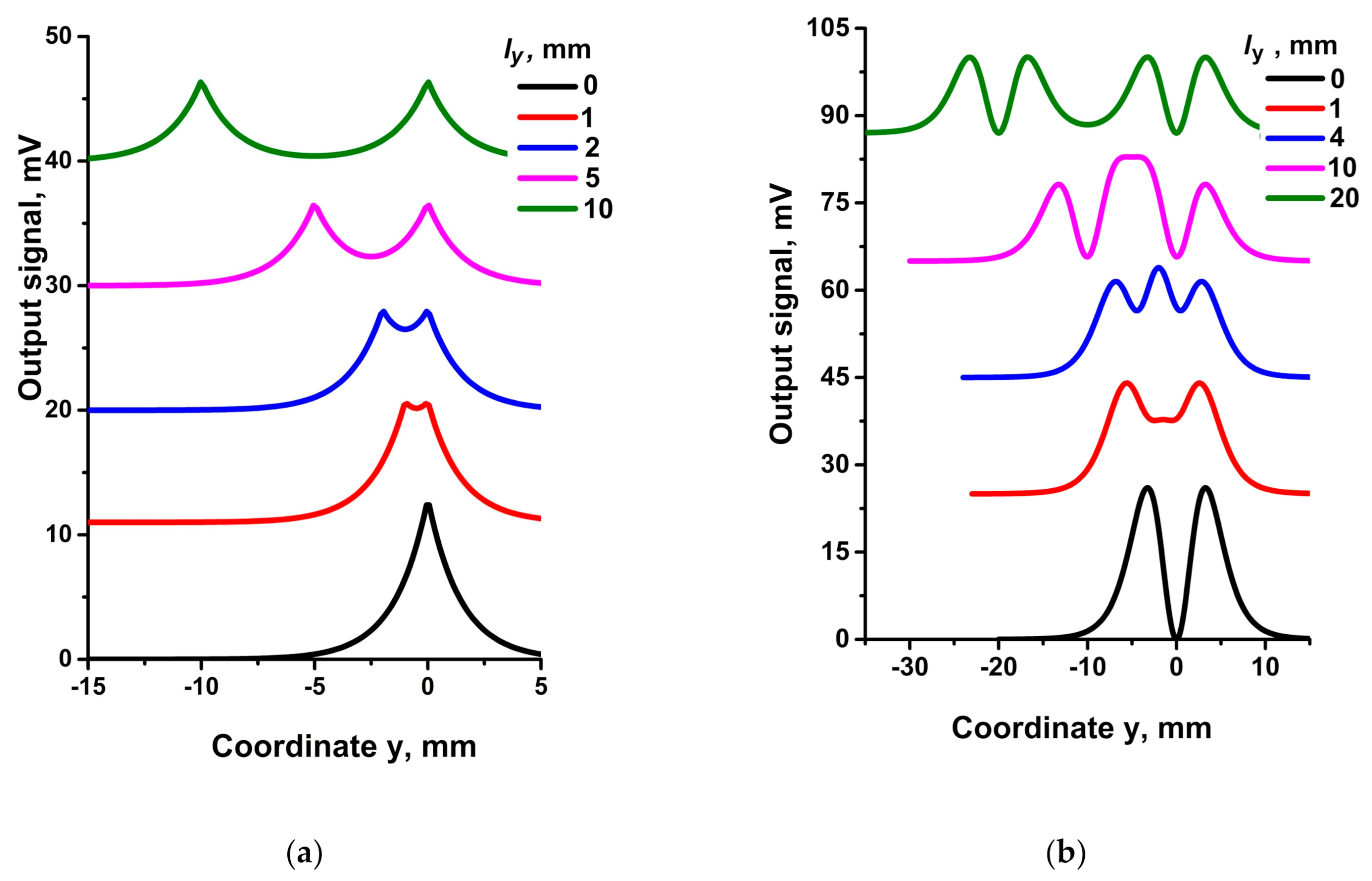
Figure 8 illustrates the shapes of output signals for a set of the bridge size in y-direction, ly.
The output signals in Figure 8a are composed of two peaks in curves for ly from 1 to 10 mm. The peak at y = 0 corresponds to R1 position opposite the label while the second one at y ≠ 0 corresponds to R4 nearest the label. Separation of these peaks is determined by the value of ly; at ly = 0 the peaks merge.
The output signal in Figure 8b is composed of two pairs of peaks (curve for ly = 20 mm). A pair of peaks at y = 0 corresponds to the R1 position opposite the label, while the second pair at y ≠ 0 corresponds to R4. Separation of the centers of these pairs is determined by ly. As ly decreases, two pairs of peaks transform into three peaks (curves for ly = 1 and 4 mm), which then merge into two peaks at ly = 0.
Figure 9 illustrates the variation of the shapes for a set of the bridge size in x-direction, lx. In both panels in Figure 9a,b one can see that the curve shapes (two and three peaks) correspond to ly = 4 mm (Figure 8), which determines the peak positions. In Figure 9a, as lx increases, the height of peaks at first increases (lx = from 1 to 6 mm), and then the height decreases while the width increases (lx from 8 to 12 mm). In Figure 9b, the height of the peaks decreases and the width increases as lx increases.
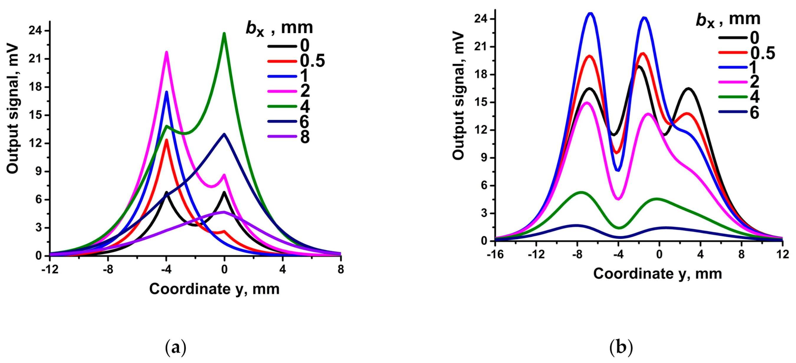
Figure 10 illustrates the dependence of the signal on bx.
The types of curves and peak positions are determined by bridge dimensions lx and ly. At bx = 0, the heights of the peaks (Figure 10a) are equal (curve for bx = 0). As bx increases, the height of the left peak increases and the height of the right peak decreases (bx from 0.5 to 2 mm). Then, the situation reverses, accompanied by widening and blurring of the peaks. The trend of changes in the picture (Figure 10b) is similar.
In general, for Figure 8, Figure 9 and Figure 10 the dimensions of the bridge ly determine the number of peaks (or pairs of peaks) and the distance between the peaks (the centers of the pairs of peaks), lx determines the magnitude of the response, and bx, the asymmetry of the response.
Let us consider the situation of the bridge also with two sensitive elements but when these elements are R1 and R3 in adjacent positions. Two variants of this situation are depicted in Figure 11.
The output signals for the cases of the elements R1 and R3 connected in series (Figure 11a) and in parallel (Figure 11b) can be expressed, respectively, as Equations (4) and (5).
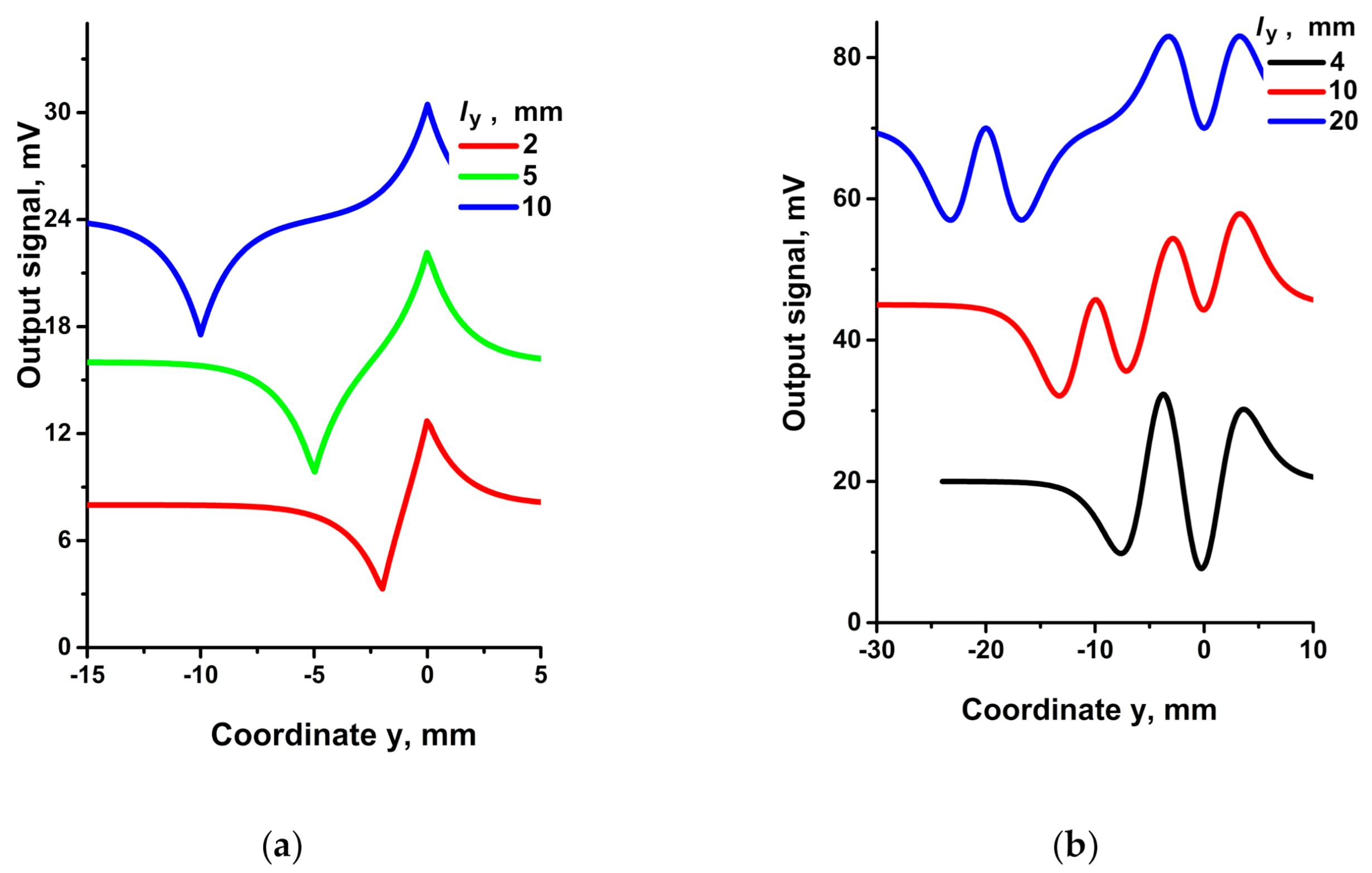
The dependences of the output signal on the sensor position along y coordinate for a number of ly parameters are shown in Figure 12.
In analogy with Figure 8a (left panel), there are also two peaks in Figure 12a (left panel). The peak at y = 0 (ly = 2 to 10 mm) corresponding to the R1 position is positive. The second peak at y ≠ 0 is negative and corresponds to the R3 position. The distance between these peaks is determined by ly for large ly. For small ly, the peaks partially compensate each other (curve ly = 2 mm), their heights diminish, and distance between them is already not equal to ly.
The dependences in Figure 12b (right panel) are similar to those in the left panel, but they concern not a single peak but pair of peaks. The positive pair of peaks at y = 0 corresponds to the R1 position, while the negative pair at y ≠ 0 corresponds to R3. The distance between the centers of these pairs is determined by ly for large ly. For small ly, the peaks partially compensate each other but in a more complex manner than in the left panel, which leads to curves of complex waveforms.
4. Conclusions
Wheatstone bridge configurations of clusters of SV sensors moving in the 3D field of a magnetic label were considered as a sensor of the magnetic field of the label. Potentially, the WB network is a more favorable device than a single SV sensor, offering higher sensitivity to a weak magnetic field and to a weak space variation of the magnetic field. That is an important feature of WB-like sensors in many applications, including the localization and positioning of a moving magnetic object.
WB network output signals were considered for different bridge sizes, numbers of sensitive elements, and orientations with respect to the label.
We have demonstrated that the WB output signal, as a function of approach distance to the label, strongly depends on several factors. First is the trajectory of the sensor, i.e., the height and width of the signal strongly depend on not only the distance of the nearest approach of the sensor to the label, the so-called impact parameter, but also the position of the line of motion with respect to the geometry and orientation of the label.
The design and parameters of the WB sensor are a second factor. Here we considered WB-like sensors of rectangular design with four SV elements, balanced in a no-field environment, with one-of-four or two-of-four sensitive SV elements and the other SV elements protected from the influence of a magnetic field. We have shown that the shape and power of the output signal critically depend on the configuration of the sensitive and protected WB arms, the size of the sensor, the number (one or two) of sensitive elements, and spacing between the sensitive arms.
A third factor is the orientation of the WB sensor with respect to the label. We have demonstrated that the response of the sensor is crucially dependent on the initial orientation of the WB basic plane and magnetic moments of the sensitive elements within the plane.
Calculations provided new information on a WB-like SV sensor manifold response to the nonhomogeneous magnetic field of an object. This information can be used to design positioning devices for a variety of applications, including the localization and positioning of a moving magnetic object.
Author Contributions
Software, G.V.B.; validation, N.G.C., I.O.D., M.G.K., A.V.M., and I.L.R.; investigation, G.V.B., M.G.K., and I.L.R.; supervision, N.G.C.; All authors have read and agreed to the published version of the manuscript.
Funding
This research received no external funding.
Institutional Review Board Statement
Not applicable.
Informed Consent Statement
Not applicable.
Data Availability Statement
Not applicable.
Conflicts of Interest
The authors declare no conflict of interest.
References
- Grosz, A.; Haji-Sheikh, M.J. High Sensitivity Magnetometers. In Smart Sensors, Measurement and Instrumentation 19; Mukhopadhyay, S.C., Ed.; Springer Nature Switzerland AG: Cham, Switzerland, 2017; p. 576. [Google Scholar] [CrossRef]
- Murzin, D.; Mapps, D.J.; Levada, K.; Belyaev, V.; Omelyanchic, A.; Panina, L.; Rodionova, V. Ultrasensitive Magnetic Field Sensors for Biomedical Applications. Sensors 2020, 20, 1569. [Google Scholar] [CrossRef] [PubMed] [Green Version]
- Zheng, C.; Zhu, K.; De Freitas, S.C.; Chang, J.Y.; Davies, J.E.; Eames, P.; Freitas, P.P.; Kazakova, O.; Kim, C.; Leung, C.W.; et al. Magnetoresistive Sensor Development Roadmap (Non-Recording Applications). IEEE Trans. Magn. 2019, 55, 0800130. [Google Scholar] [CrossRef] [Green Version]
- Pannetier-Lecoeur, M.; Fermon, C.; Goff, G.L.; Simola, J.; Kerr, E. Femtotesla magnetic field measurement with magnetoresistive sensors. Science 2004, 304, 1648–1650. [Google Scholar] [CrossRef] [PubMed]
- Baselt, D.R.; Lee, G.U.; Natesan, M.; Metzger, S.W.; Sheehan, P.E.; Colton, R.J. A biosensor based on magnetoresistance technology. Biosens. Bioelectron. 1998, 13, 731–739. [Google Scholar] [CrossRef]
- Germano, J.; Martins, V.C.; Cardoso, F.A.; Almeida, T.M.; Sousa, L.; Freitas, P.P.; Piedade, M.S. A portable and autonomous magnetic detection platform for biosensing. Sensors 2009, 9, 4119–4137. [Google Scholar] [CrossRef] [Green Version]
- Graham, D.L.; Ferreira, H.A.; Freitas, P.P. Magnetoresistive-based biosensors and biochips. Trends Biotechnol. 2004, 22, 455–462. [Google Scholar] [CrossRef]
- Parkin, S.S.P. Flexible giant magnetoresistance sensors. Appl. Phys. Lett. 1996, 69, 3092–3094. [Google Scholar] [CrossRef]
- Uhrmann, T.; Bär, L.; Dimopoulos, T.; Wiese, N.; Rührig, M.; Lechner, A. Magnetostrictive GMR sensor on flexible polyimide substrates. J. Magn. Magn. Mater. 2006, 307, 209–211. [Google Scholar] [CrossRef]
- Karnaushenko, D.; Makarov, D.; Yan, C.; Streubel, R.; Schmidt, O. Printable giant magnetoresistive devices. Adv. Mater. 2012, 24, 4518–4522. [Google Scholar] [CrossRef]
- Gaspar, J.; Fonseca, H.; Paz, E.; Martins, M.; Valadeiro, J.; Cardoso, S.; Ferreira, R.; Freitas, P.P. Flexible magnetoresistive sensors designed for conformal integration. IEEE Trans. Magn. 2017, 53, 5300204. [Google Scholar] [CrossRef]
- Ausserlechner, U. The optimum layout for giant magneto-resistive angle sensors. IEEE Sens. J. 2010, 10, 1571–1582. [Google Scholar] [CrossRef]
- Hahn, R.; Schmidt, T.; Slatter, R.; Olberts, B.; Romera, F. Magnetoresistive angular sensors for space applications: Results of breadboard and EQM testing and lessons learned. In Proceedings of the 17th European Space Mechanism and Tribology Symposium (ESMATS), Hatfield, UK, 20–22 September 2017; pp. 1–6. [Google Scholar]
- Díaz-Michelena, M. Small Magnetic Sensors for Space Applications. Sensors 2009, 9, 2271–2288. [Google Scholar] [CrossRef]
- Sun, X.; Lui, K.S.; Wong, K.K.; Lee, W.K.; Hou, Y.; Huang, Q.; Pong, P.W. Novel application of magnetoresistive sensors for highvoltage transmission-line monitoring. IEEE Trans. Magn. 2011, 47, 2608–2611. [Google Scholar] [CrossRef] [Green Version]
- Liu, L.Y.; Jiang, S.B.; Yeh, T.L.; Yeh, H.C.; Liu, J.Y.; Hsu, Y.H.; Ji-Yi, P. The magneto-resistive magnetometer of BCU on the Tatiana-2 satellite. Terr. Atmos. Ocean Sci. 2012, 23, 317–326. [Google Scholar] [CrossRef] [Green Version]
- Yong, O.; He, J.; Hu, J.; Wang, S.X. A current sensor based on the giant magnetoresistance effect: Design and potential smart grid applications. Sensors 2012, 12, 15520–15541. [Google Scholar] [CrossRef]
- Zhu, K.; Han, W.; Lee, W.K.; Pong, P.W.T. On-site non-invasive current monitoring of multi-core underground power cables with a magnetic-field sensing platform at a substation. IEEE Sens. J. 2017, 17, 1837–1848. [Google Scholar] [CrossRef]
- Caruso, M.J. Applications of magnetoresistive sensors in navigation systems. Prog. Technol. 1998, 72, 159–168. [Google Scholar] [CrossRef] [Green Version]
- Lai, Y.-C.; Jan, S.-S.; Hsiao, F.-B. Development of a low-cost attitude and heading reference system using a three-axis rotating platform. Sensors 2010, 10, 2472–2491. [Google Scholar] [CrossRef] [Green Version]
- Michelena, M.D.; Arruego, I.; Oter, J.; Guerrero, H. COTS-based wireless magnetic sensor for small satellites. IEEE Trans. Aerosp. Electron. Syst. 2010, 46, 542–557. [Google Scholar] [CrossRef]
- Sanz, R.; Fernández, A.B.; Dominguez, J.A.; Martín, B.; Michelena, M.D. Gamma irradiation of magnetoresistive sensors for planetary exploration. Sensors 2012, 12, 4447–4465. [Google Scholar] [CrossRef]
- Arias, S.I.R.; Muñoz, D.R.; Cardoso, S.; Ferreira, R.; de Freitas, P.J.P. Total ionizing dose (TID) evaluation of magnetic tunnel junction (MTJ) current sensors. Sens. Actuators. A Phys. 2015, 225, 119–127. [Google Scholar] [CrossRef]
- Baibich, M.N.; Broto, J.M.; Fert, A.; Nguyen Van Dau, F.; Petroff, F.; Etienne, P.; Creuzet, G.; Friederich, A.; Chazelas, J. Giant magnetoresistance of (001)Fe/(001)Cr magnetic superlattices. Phys. Rev. Lett. 1988, 61, 2472–2475. [Google Scholar] [CrossRef] [Green Version]
- Binasch, G.; Grünberg, P.; Saurenbach, F.; Zinn, W. Enhanced magnetoresistance in layered magnetic structures with antiferromagnetic interlayer exchange. Phys. Rev. B Condens. Matter 1989, 39, 4828. [Google Scholar] [CrossRef] [Green Version]
- Reig, C.; de Freitas, S.C. Giant Magnetoresistance (GMR) Sensors. In Smart Sensors, Measurement and Instrumentation; Mukhopadhyay, S.C., Ed.; Springer: Berlin/Heidelberg, Germany, 2013; Volume 6, p. 300. [Google Scholar] [CrossRef]
- Kools, J.C.S. Exchange-Biased Spin-Valves for Magnetic Storage. IEEE Trans. Mag. 1996, 32, 3165–3184. [Google Scholar] [CrossRef]
- Stoner, E.C.; Wohlfarth, E.P. A mechanism of magnetic hysteresis in heterogeneous alloys. Phil. Trans. Roy. Soc. 1948, 240, 599–642. [Google Scholar] [CrossRef]
- Szasz, K.; Bakonyi, I. Modeling the magnetoresistance vs. field curves of GMR multilayers with antiferromagnetic and/or orthogonal coupling by assuming single-domain state and coherent rotation. J. Spintron. Magn. Nanomater. 2012, 1, 157–167. [Google Scholar] [CrossRef]
- Reig, C.; Cubells-Beltran, M.D.; Munoz, D.R. Magnetic Field Sensors Based on Giant Magnetoresistance (GMR) Technology: Applications in Electrical Current Sensing. Sensors 2009, 9, 7919–7942. [Google Scholar] [CrossRef]
- Kurenkov, A.S.; Babaytsev, G.V.; Chechenin, N.G. An origin of asymmetry of giant magnetoresistance loops in spin valves. J. Magn. Magn. Mater. 2019, 470, 147–150. [Google Scholar] [CrossRef]
- Bukunov, K.; Babaitsev, G.; Chechenin, N. Modeling of magnetic label field sensing by GMR structure. EPJ Web Conf. 2018, 185, 01001. [Google Scholar] [CrossRef]
- Babaitsev, G.V.; Chechenin, N.G.; Dzhun, I.O.; Kozin, M.G.; Romashkina, I.L. GMR effect in nonhomogeneous magnetic field. J. Phys. Conf. Ser. 2019, 1389, 012145. [Google Scholar] [CrossRef]
- Babaitsev, G.V.; Chechenin, N.G.; Dzhun, I.O.; Romashkina, I.L.; Kozin, M.G.; Makunin, A.V. Spin-valve sensor in the magnetic field of a moving label. Moscow Univ. Phys. Bull 2021. In Press. [Google Scholar]
- Bruckner, F.; Bergmair, B.; Brueckl, H.; Palmesi, P.; Buder, A.; Satz, A.; Suess, D. A device model framework for magnetoresistive sensors based on the Stoner–Wohlfarth model. J. Magn. Magn. Mater. 2015, 381, 344–349. [Google Scholar] [CrossRef] [Green Version]
Figure 1.
Schematic representation of a SV layer structure: BL denotes a buffer layer; AF, antiferromagnetic layer; PF, pinned ferromagnetic layer; NM, non-magnetic layer; FF, free ferromagnetic layer; and PL, protective layer.
Figure 1.
Schematic representation of a SV layer structure: BL denotes a buffer layer; AF, antiferromagnetic layer; PF, pinned ferromagnetic layer; NM, non-magnetic layer; FF, free ferromagnetic layer; and PL, protective layer.

Figure 2.
An example of y-dependence of the magnetic field components along the trajectory {x = −1, y = var, z = 6 mm} for a cuboid label.
Figure 2.
An example of y-dependence of the magnetic field components along the trajectory {x = −1, y = var, z = 6 mm} for a cuboid label.

Figure 3.
Wheatstone bridge circuit. A, B are input, C, D—output contact points, R1–R4 are resistances.
Figure 3.
Wheatstone bridge circuit. A, B are input, C, D—output contact points, R1–R4 are resistances.

Figure 4.
Bridge circuits with 1 (a) and 2 (b) sensing arms, marked with red arrows indicating structures that change their resistance.
Figure 4.
Bridge circuits with 1 (a) and 2 (b) sensing arms, marked with red arrows indicating structures that change their resistance.

Figure 5.
Mutual orientation and location of the moving bridge and magnetic label (grey squares). The direction of magnetization M for sensitive element R1 in the bridge (red arrow) is either parallel to y (a) or parallel to x (b), i.e., either parallel or perpendicular to the movement direction of the bridge (green arrow). Red point in the center of the gray square symbolizes z-direction of magnetization for the label. Red lines with arrows around the labels show schematic projections of the label magnetic field onto the xy plane.

Figure 6.
Output signals of the SV bridges with one sensitive R1 element as a function of the position along the y coordinate. Bridge orientations correspond to M||y (Figure 5a) on the left panel, (i.e., a,c) and M||x (Figure 5b) on the right panel,(i.e., b,d). Curves in (a,b) correspond to the trajectories of R1, respectively, {x = x0 = 0.5; 1; 2; 5 mm, y = var; z = z0 = 6 mm}, and in (c,d) correspond to the R1 trajectories, respectively { x = x0 = 1 mm, y = var, z0 = z = 6; 6.5; 7; 8; 10 mm}.

Figure 7.
Mutual orientation and location of the moving bridge and magnetic label. lx, ly are the distances between sensor elements along the x and y axes, and bx, bz (the latter is not shown) are impact parameters (nearest approach distance) in x and z directions. The direction of magnetization for sensitive elements R1 and R4 of the bridge is parallel (a) or perpendicular (b) to the movement direction, shown by green arrow.

Figure 8.
Representative responses of two bridges at different ly = 0; 1; 2; 5; 10 mm ((a), bridge orientations correspond to Figure 7a), and ly = 0; 1; 4, 10, 20 mm ((b), bridge orientations correspond to Figure 7b), at lx = 2 mm, bx = 0, bz = 6 mm. R1 and R4 are the sensitive elements. Curves are shifted along the vertical axis for better readability.

Figure 9.
Response of two bridges at different lx = 1; 2; 3; 6; 8; 10; 12 mm ((a), bridge orientations correspond to Figure 7a), and lx = 1; 2; 3; 6; 8; 10 mm ((b), bridge orientations correspond to Figure 7b), at ly = 4 mm, bx = 0, bz = 6 mm. R1 and R4 are the sensitive elements.

Figure 10.
Response of two bridges at different bx = 0; 0.5; 1; 2; 4; 6; 8 mm ((a), bridge orientations correspond to Figure 7a), and bx = 0; 0.5; 1; 2; 4; 6 mm ((b), bridge orientations correspond to Figure 7b). For both orientations lx = 2 mm, ly = 4 mm, bz = 6 mm. R1 and R4 are the sensitive elements.

Figure 11.
Mutual orientation and location of the moving bridge and magnetic label. R1 and R3 are the sensitive elements of the bridge, their direction of magnetization is parallel (a) or perpendicular (b) to the movement direction of the bridge.
Figure 11.
Mutual orientation and location of the moving bridge and magnetic label. R1 and R3 are the sensitive elements of the bridge, their direction of magnetization is parallel (a) or perpendicular (b) to the movement direction of the bridge.

Figure 12.
Response of two bridges at different ly = 2; 5; 10 mm ((a), bridge orientations correspond to Figure 11a), and ly = 4, 10; 20 mm ((b), bridge orientations correspond to Figure 11b), at lx = 2 mm, bx = 0, bz = 6 mm. R1 and R3 are the sensitive elements with their direction of magnetization parallel (a) or perpendicular (b) to the movement direction of the bridge. Curves are shifted along the vertical axis for better readability.

Publisher’s Note: MDPI stays neutral with regard to jurisdictional claims in published maps and institutional affiliations. |
© 2021 by the authors. Licensee MDPI, Basel, Switzerland. This article is an open access article distributed under the terms and conditions of the Creative Commons Attribution (CC BY) license (https://creativecommons.org/licenses/by/4.0/).
Share and Cite
MDPI and ACS Style
Babaytsev, G.V.; Chechenin, N.G.; Dzhun, I.O.; Kozin, M.G.; Makunin, A.V.; Romashkina, I.L. Clusters of Spin Valve Sensors in 3D Magnetic Field of a Label. Sensors 2021, 21, 3595. https://0-doi-org.brum.beds.ac.uk/10.3390/s21113595
AMA Style
Babaytsev GV, Chechenin NG, Dzhun IO, Kozin MG, Makunin AV, Romashkina IL. Clusters of Spin Valve Sensors in 3D Magnetic Field of a Label. Sensors. 2021; 21(11):3595. https://0-doi-org.brum.beds.ac.uk/10.3390/s21113595
Chicago/Turabian StyleBabaytsev, Georgy V., Nikolay G. Chechenin, Irina O. Dzhun, Mikhail G. Kozin, Alexey V. Makunin, and Irina L. Romashkina. 2021. "Clusters of Spin Valve Sensors in 3D Magnetic Field of a Label" Sensors 21, no. 11: 3595. https://0-doi-org.brum.beds.ac.uk/10.3390/s21113595
Note that from the first issue of 2016, this journal uses article numbers instead of page numbers. See further details here.