
Real-Time Path Planning Based on Harmonic Functions under a Proper Generalized Decomposition-Based Framework

 ,
,  ,
,  , and
, and 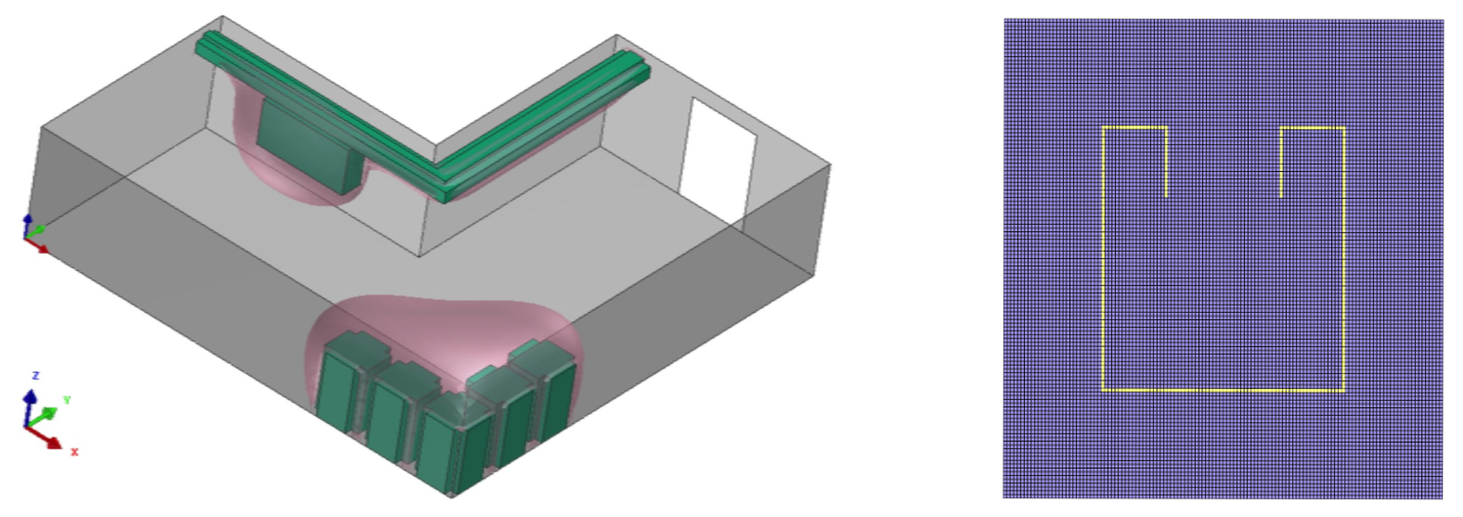
Abstract
:1. Introduction
2. Previous Knowledge
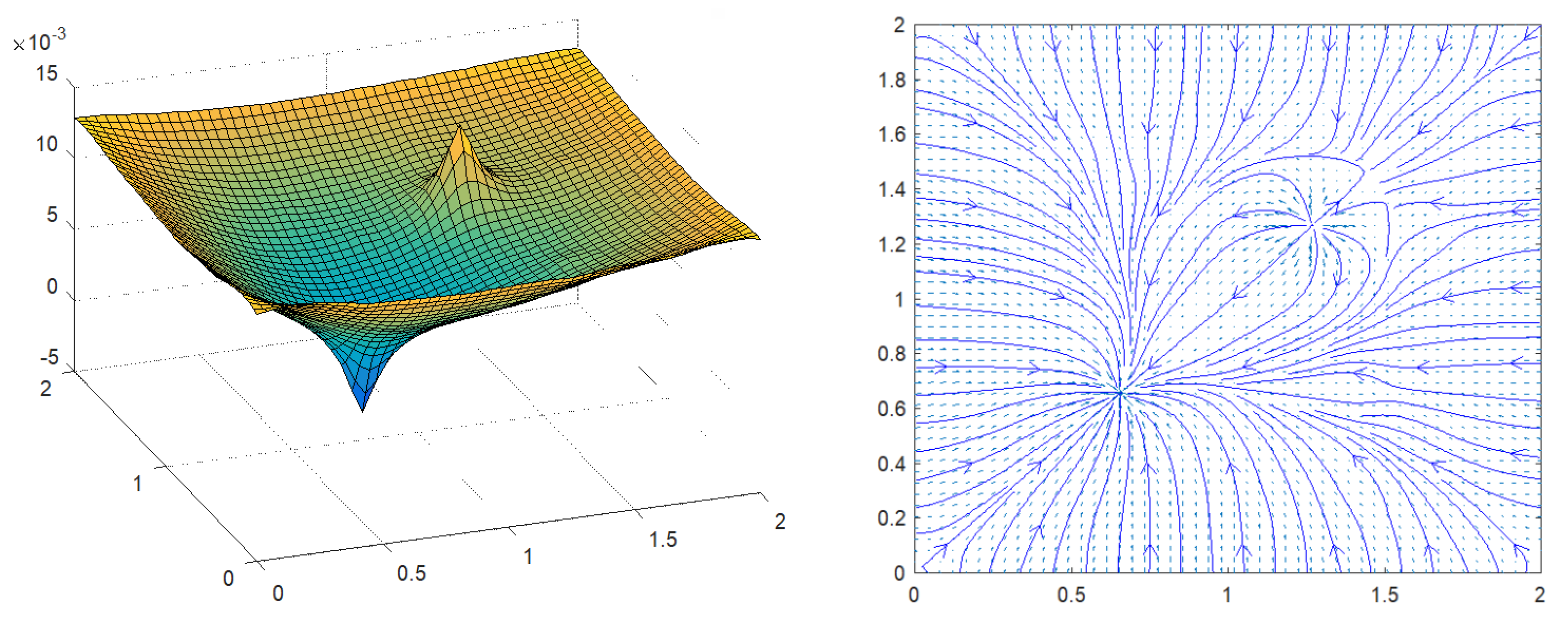
2.1. Potential Flow Theory
2.2. Source Term Definition
2.3. A PGD-Vademecum Solution
2.4. Meshing Constraints to Guarantee Free-of-Deadlocks Solutions
- The mesh of must be cell-centred with the and meshes. This means that the physical positions of the nodes and must also exist in the mesh. It is obvious as all the robot origins and destinations must appear on the map. In addition, the dimensions of and can be much smaller than the dimension of , since all the start (and goal) positions could be separated a moderated distance (0.5 m, for example) while the navigation map must be accurate (with separation between nodes of a few cm).
- The mesh of must be staggered with the mesh.
3. Simulated Validation. Construction of the PGD-Vademecum in Complex and Real Environments
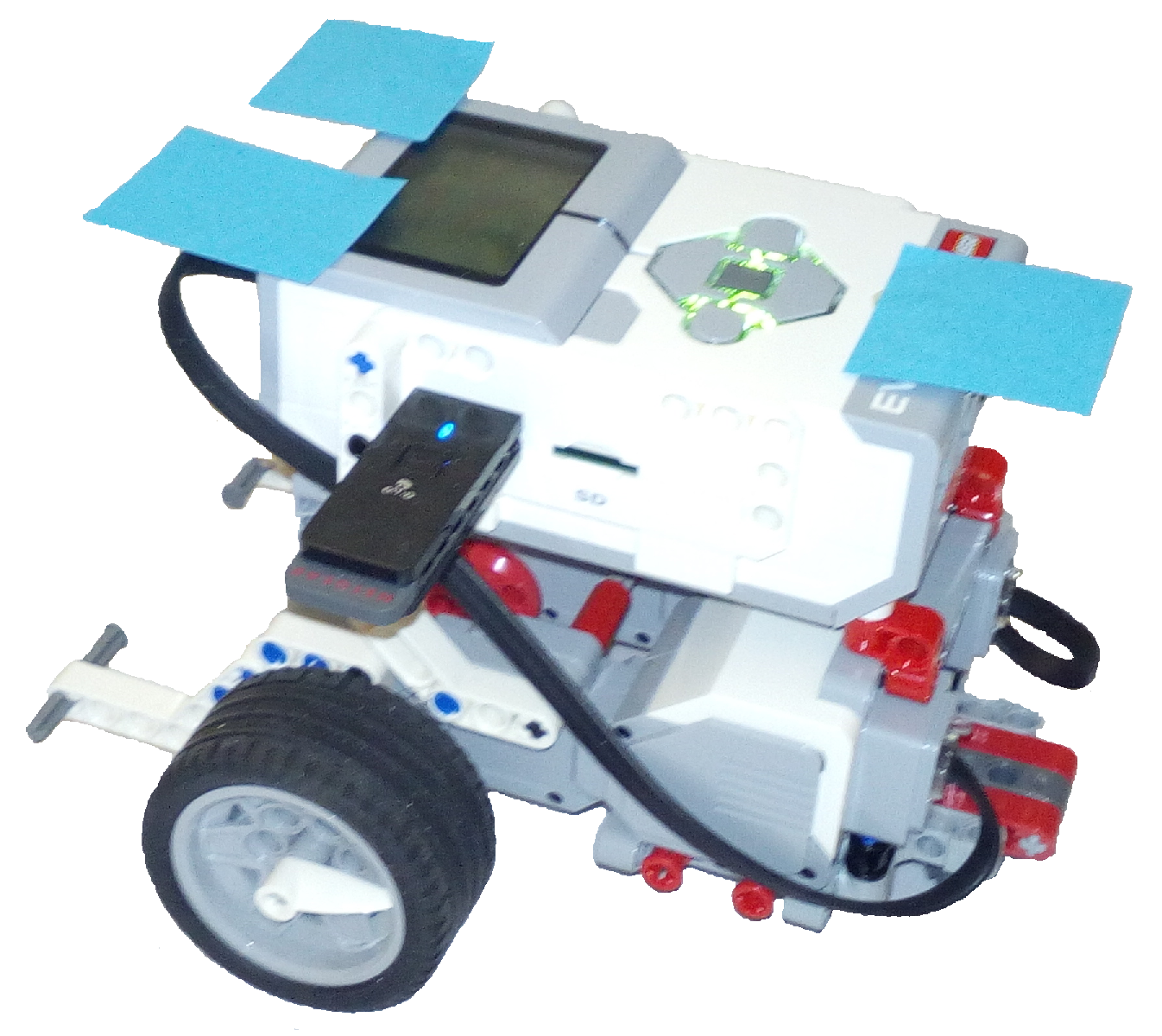
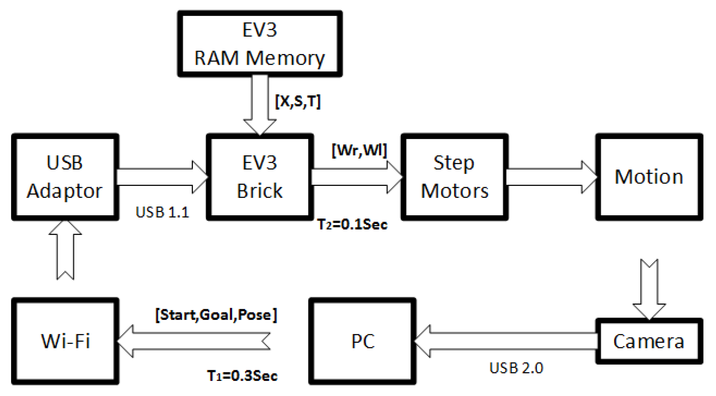
4. Experimental Validation. PGD-Vademecum in a Lego ®Mindstorms
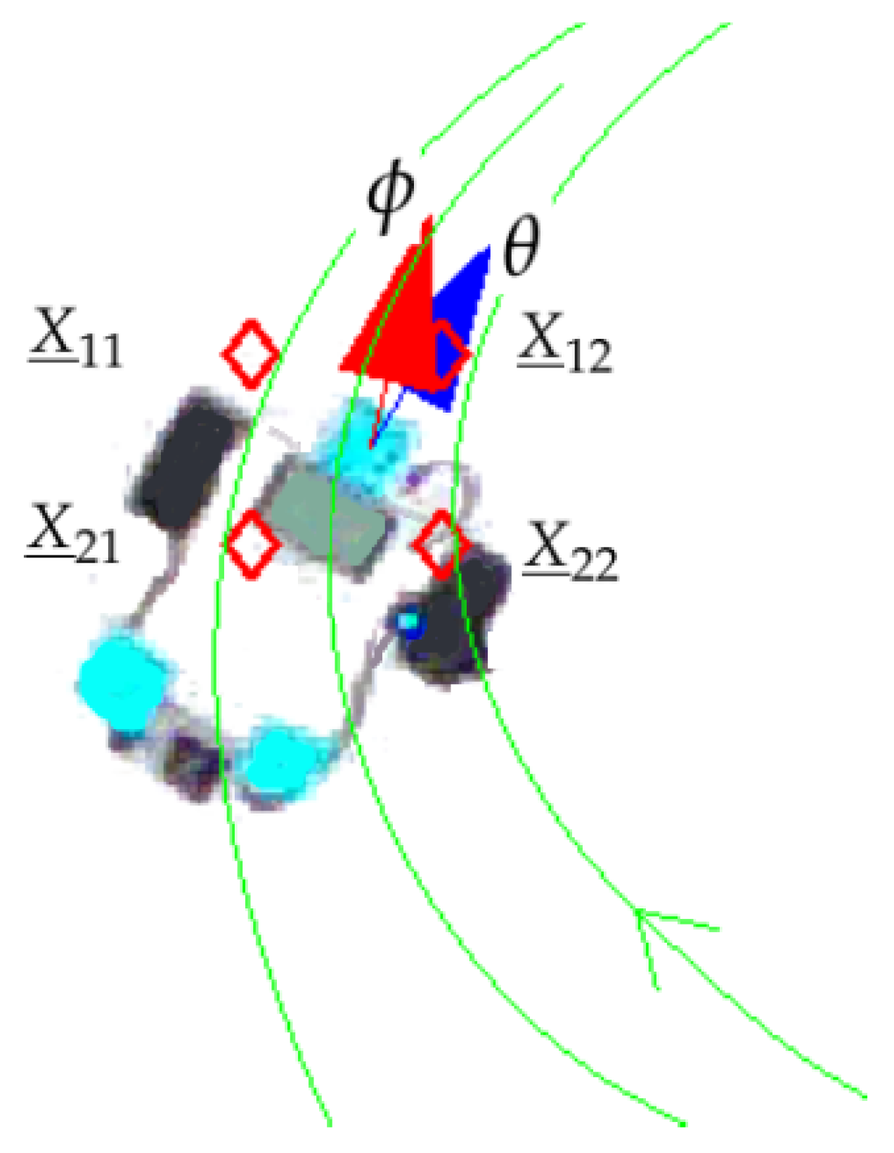
4.1. PGD-Vademecum to Compute the Wheels Velocities
4.2. Experimental Tests
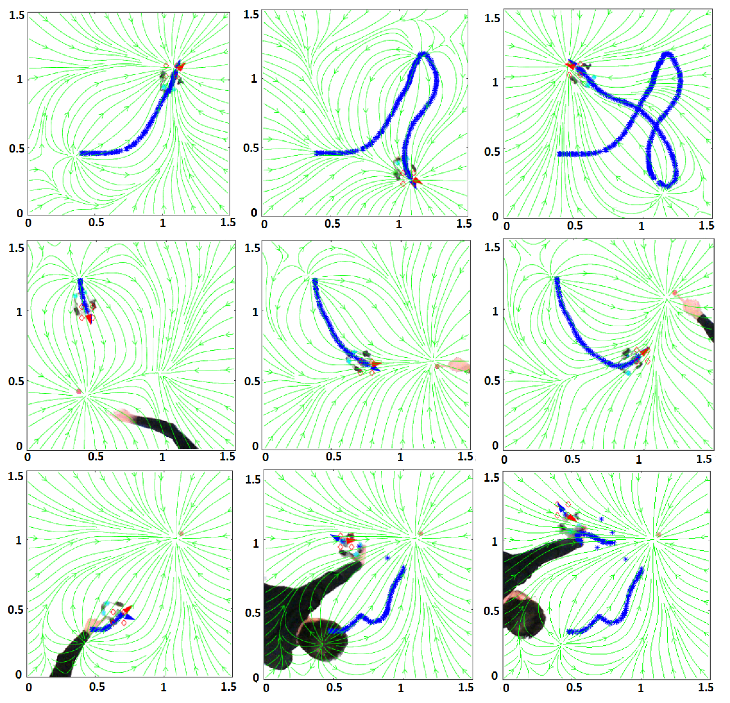
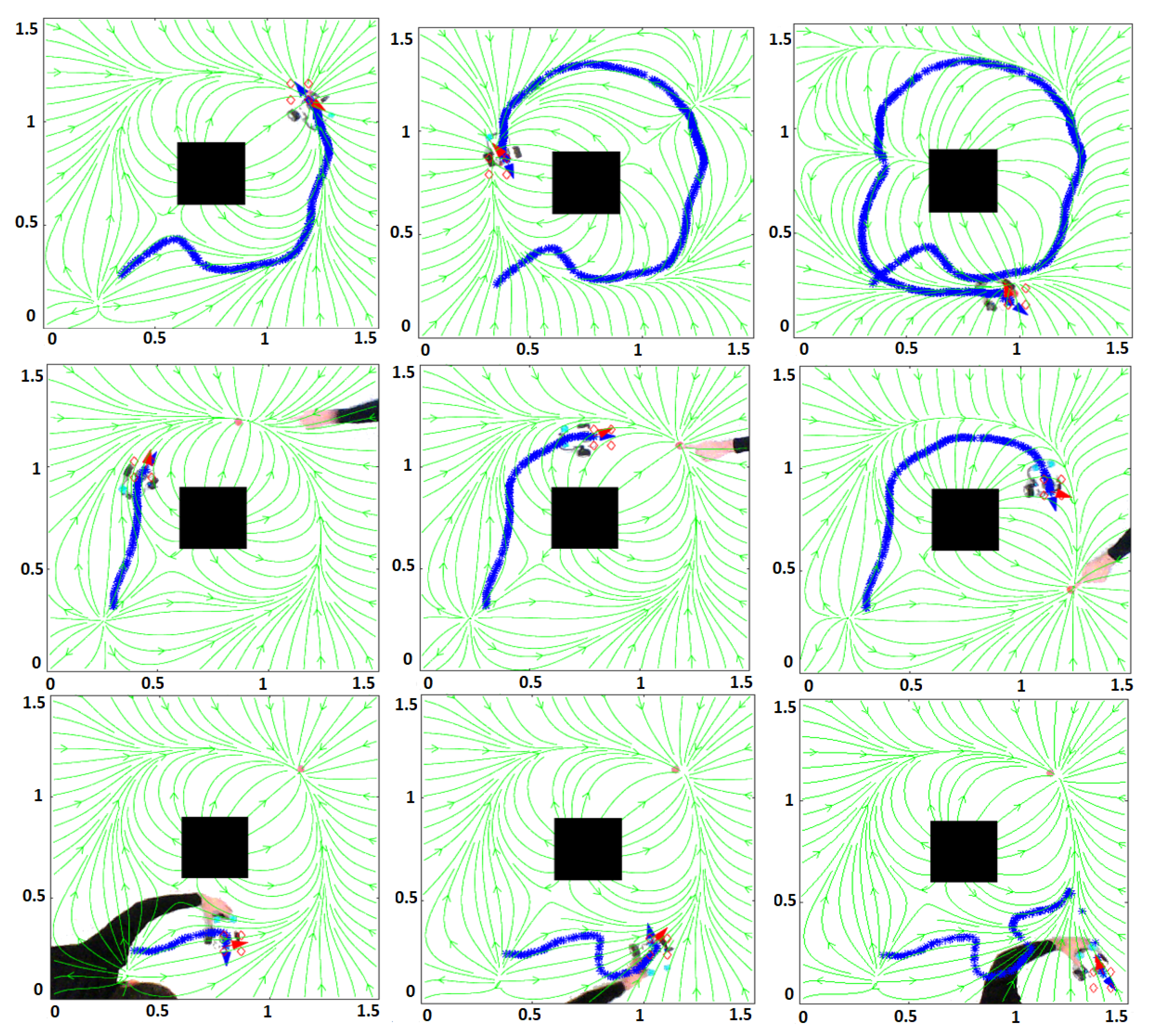
- Test 1: Point to Point.This test shows that the PGD-vademecum could cover all the possible start and goal combinations for the vehicle position. The test procedure is as follows: the red disk is thrown to the scene, falling into an arbitrary position, and the vehicle must reach the red disk (goal); once the robot reaches the goal, the red disk is thrown to another arbitrary position.
- Test 2: Dynamic Goal.This test demonstrates that the robot does not need additional computation when the goal changes before the robot reaches it, unlike in [18] where, if the goal changes while the robot is following a particular streamline, a new FEM simulation must be executed and the robot has to wait for the new FEM simulation solution. The test procedure is the following: the red disk is thrown to the scene falling into an arbitrary position; the red disk (goal) changes in real-time (due to external causes) forcing the robot to adjust its target while navigating the environment.
- Test 3: Perturbations.This tests demonstrates the robustness of the potential field approach for each particular PGD-vademecum solution. For that purpose, the robot is perturbed, changing its pose before reaching the goal. The procedure of this test is as follows: the red disk is thrown to the scene falling into an arbitrary position; the robot pose is manually changed to another arbitrary pose, forcing it to recompute its trajectory in real-time.
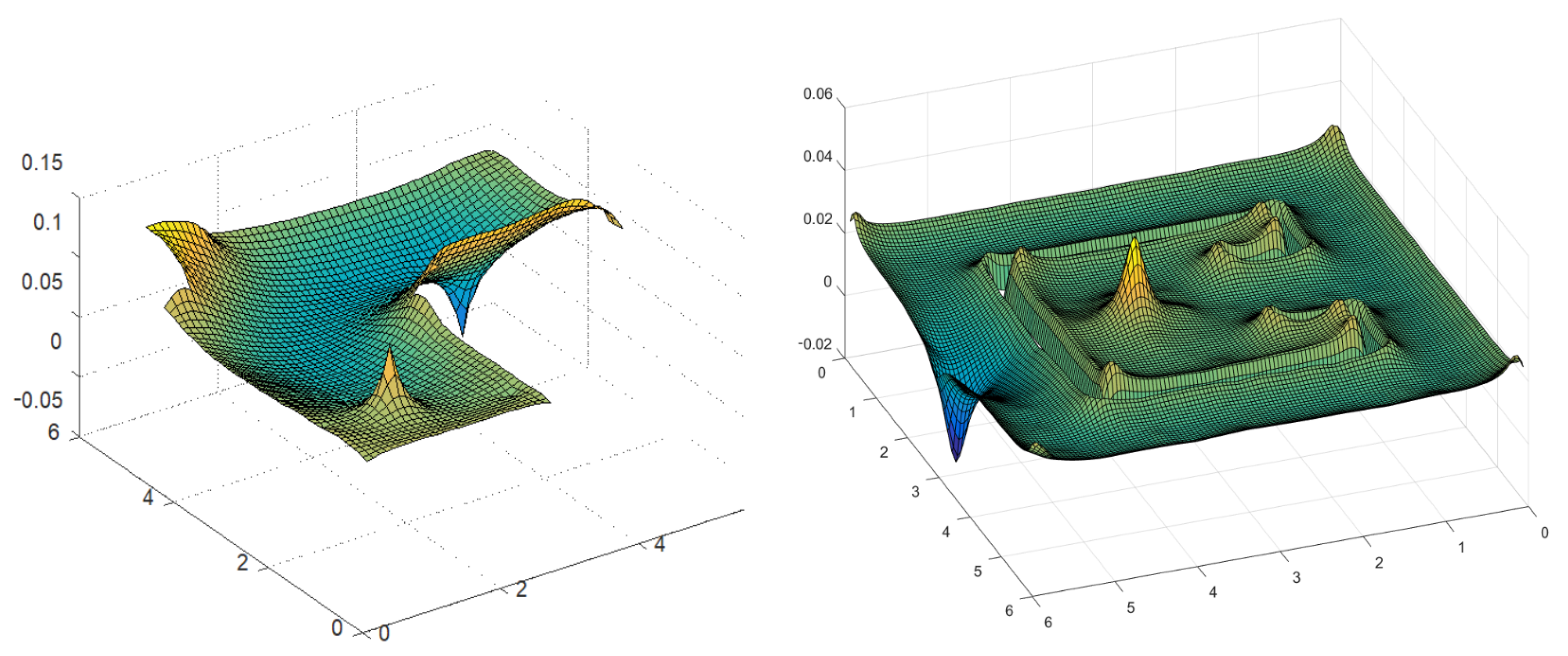
- Modality A: Without static obstacles.In this modality, the robot navigates a square environment of 1.5 × 1.5 m discretized with nodes. The precomputed PGD-Vademecum has the following parameters: , and .
- Modality B: With a static obstacle.In this modality, the robot navigates a 1.5 m × 1.5 m square with a square static obstacle of 0.3 × 0.3 m located at the centre of the environment. This would be a common situation for an autonomous robot moving in a house, a parking lot, a field with trees, etc., where the map contains static obstacles, and the robot has to skirt them. The environment is also discretized with nodes. The precomputed PGD-vademecum has the following parameters: and and . The generation of static obstacles only involves the assignation of boundary conditions to the nodes belonging to each static obstacle. It allows the construction of any configuration map.
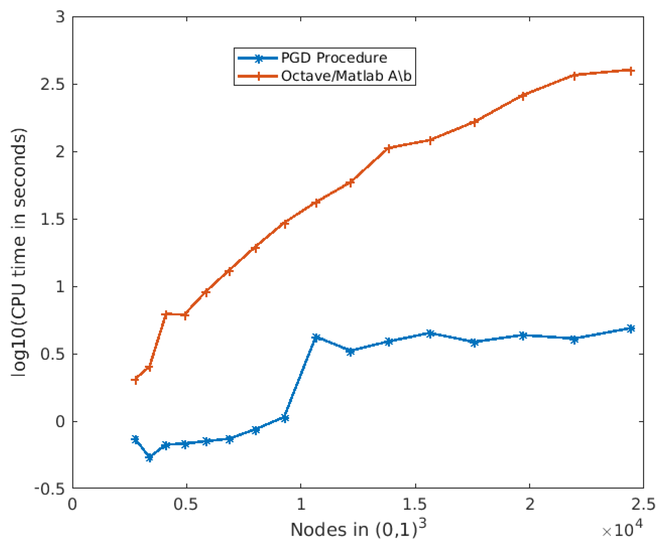
5. Time and Memory Complexity of the Method
6. Conclusions and Future Work
Author Contributions
Funding
Conflicts of Interest
References
- Reif, J.H. Complexity of the mover’s problem and generalizations. In Proceedings of the 20th Annual Symposium on Foundations of Computer Science, San Juan, Puerto Rico, 29–31 October 1976; pp. 421–427. [Google Scholar]
- Kavraki, L.E.; LaValle, S. Chapter 5. Motion Planning. In Handbook of Robotics; Siciliano, K., Ed.; Springer: Berlin/Heidelberg, Germany, 2008. [Google Scholar]
- González, D.; Pérez, J.; Milanés, V.; Nashashibi, F. A Review of Motion Planning Techniques for Automated Vehicles. IEEE Trans. Intell. Transp. Syst. 2016, 17, 1135–1145. [Google Scholar] [CrossRef]
- Khatib, O. Real-time obstacle avoidance for manipulators and mobile robots. Int. J. Robot Res. 1986, 5, 90–98. [Google Scholar] [CrossRef]
- Rimon, E.; Koditschek, D. Exact robot navigation using artificial potential functions. IEEE Trans. Robot. Autom. 1992, 8, 501–518. [Google Scholar] [CrossRef] [Green Version]
- Lazarowska, A. Discrete Artificial Potential Field Approach to Mobile Robot Path Planning. IFAC-PapersOnLine 2019, 52, 277–282. [Google Scholar] [CrossRef]
- Pengwei, W.; Song, W.; Liang, L.; Binbin, S.; Shuo, C. Obstacle Avoidance Path Planning Design for Autonomous Driving Vehicles Based on an Improved Artificial Potential Field Algorithm. Energeies 2019, 12, 2342. [Google Scholar]
- Xinping, G.; Mengxin, H.; Weishuai, Z.; Gang, X.; Guohua, Z.; Yunpeng, H. Intelligent Vehicle Path Planning Based on Improved Artificial Potential Field Algorithm. In Proceedings of the IEEE International Conference on High Performance Big Data and Intelligent Systems (HPBD&IS), Shenzhen, China, 9–11 May 2019; pp. 104–109. [Google Scholar]
- Kipp, A.; Schneider, S. Applied Social Robotics—Building Interactive Robots with LEGO Mindstorms. In Robotics in Education: Advances in Intelligent Systems and Computing; Merdan, M., Lepuschitz, W., Koppensteiner, G., Balogh, R., Eds.; Springer: Cham, Switzerland, 2017; Volume 457, pp. 29–40. [Google Scholar]
- Chen, W.; Zhang, T.; Yanbiao, Z. Mobile robot path planning based on social interaction space in social environment. Int. J. Adv. Robot. Syst. 2018, 15, 1–10. [Google Scholar] [CrossRef] [Green Version]
- Calderita, L.V.; Vega, A.; Bustos, P.; Nuñez, P. Social Robot Navigation adapted to Time-dependent Affordance Spaces: A Use Case for Caregiving Centers. In Proceedings of the IEEE International Workshop on Robot and Human Communication (ROMAN), Naples, Italy, 31 August–4 September 2020; Volume 15, pp. 944–949. [Google Scholar]
- Kim, J.; Khosla, P. Real-time obstacle avoidance using harmonic potencial functions. IEEE Trans. Robot. Autom. 1992, 8, 338–349. [Google Scholar] [CrossRef] [Green Version]
- Zhachmanoglou, E.; Thoe, D.W. Introduction to Partial Differential Equations with Applications; Dover Publications, Inc.: New York, NY, USA, 1986. [Google Scholar]
- Connolly, C.I.; Grupen, R. The Application of Harmonic functions to Robotics. J. Robot. Syst. 1993, 10, 931–946. [Google Scholar] [CrossRef] [Green Version]
- Garrido, S.; Moreno, L.; Blanco, D.; Martín Monar, F. Robotic Motion Using Harmonic Functions and Finite Elements. J. Intell. Robot. Syst. 2010, 59, 57–73. [Google Scholar] [CrossRef] [Green Version]
- Connolly, C.I.; Burns, J.B.; Weiss, R. Path planning using Laplace’s equation. In Proceedings of the IEEE International Conference on Robotics and Automation, Cincinnati, OH, USA, 13–18 May 1990; pp. 2102–2106. [Google Scholar]
- Waydo, S.; Murray, R.M. Vehicle motion planning using stream functions. In Proceedings of the 2003 IEEE International Conference on Robotics and Automation (Cat. No.03CH37422), Taipei, Taiwan, 14–19 September 2003; Volume 2, pp. 2484–2491. [Google Scholar]
- Gingras, D.; Dupuis, E.; Payre, G.; Lafontaine, J. Path Planning Based on Fluid mechanics for mobile robots used Unstructured Terrain models. In Proceedings of the IEEE International Conference on Robotics and Automation, Anchorage, AK, USA, 3–7 May 2010. [Google Scholar]
- Saudi, A.; Sulaiman, J. Path Planing for mobile robots using 4EGSOR via Nine-Point Laplacian (4EGSOR9L) Iterative method. Int. J. Comput. Appl. 2012, 53, 38–42. [Google Scholar]
- Saudi, A.; Sulaiman, J.; Ahmad Hijazi, M.H. Robot Path Planing with EGSOR Iterative Method using Laplacian Behaviour-Based Control (LBBC). In Proceedings of the 5th International Conference on Intelligent Systems, Modelling and Simulation, Langkawi, Malaysia, 27–29 January 2014; pp. 87–91. [Google Scholar]
- Falcó, A.; Nouy, A. Proper Generalized Decomposition for Nonlinear Convex Problems in Tensor Banach Spaces. Numer. Math. 2012, 121, 503–530. [Google Scholar] [CrossRef] [Green Version]
- Chinesta, F.; Leygue, A.; Bordeu, F.; Aguado, J.V.; Cueto, E.; Gonzalez, D.; Alfaro, I.; Ammar, A.; Huerta, A. PGD-Based Computational Vademecum for Efficient Design, Optimization and Control. Arch. Comput. Methods Eng. 2013, 20, 31–49. [Google Scholar] [CrossRef]
- Chinesta, F.; Keunings, R.; Leygue, A. The Proper Generalized Decomposition for Advanced Numerical Simulations: A Primer; Springer Briefs in Applied Science and Technology; Springer: Berlin/Heidelberg, Germany, 2014. [Google Scholar]
- Montés, N.; Chinesta, F.; Falco, A.; Mora, M.C.; Hilario, L.; Nadal, E.; Duval, J.L. Towards a PGD-based Computational Vademecum for robot path planning. In Informatics in Control, Automation and Robotics, Proceedings of the ICINCO 2019, Prague, Czech Republic, 29–31 July 2019; Lecture Notes in Electrical Engineering; Gusikhin, O., Madani, K., Zaytoon, J., Eds.; Springer: Cham, Switzerland, 2020; Volume 720, pp. 1–15. [Google Scholar]
- Akishita, S.; Kawamura, S.; Hayashi, K. New navigation function utilizing hydrodynamic potential for mobile robot. In Proceedings of the IEEE International Workshop on Intelligent Motion Control, Istanbul, Turkey, 20–22 August 1990; Volume 2, pp. 413–417. [Google Scholar]
- Akishita, S.; Hisanobu, T.; Kawamura, S. Fast path planning available for moving obstacle avoidance by use of Laplace potential. In Proceedings of the IEEE/RSJ International Conference on Intelligent Robots and Systems, Yokohama, Japan, 26–30 July 1993; Volume 1, pp. 673–678. [Google Scholar]
- Guldner, J.; Utkin, V.I.; Hashimoto, H. Robot obstacle avoidance in n-dimensional space using planar harmonic artificial fields. J. Dyn. Syst. Meas. Control 1997, 119, 160–166. [Google Scholar] [CrossRef]
- Keymeulen, D.; Decuyper, J. The fluid dynamics applied to mobile robot motion: The stream field method. In Proceedings of the IEEE International Conference on Robotics and Automation, San Diego, CA, USA, 8–13 May 1994; pp. 378–385. [Google Scholar]
- Li, Z.X.; Bui, T.D. Robot path planning using Fluid Model. J. Intell. Robot. Syst. 1998, 21, 29–50. [Google Scholar] [CrossRef]
- Rosell, J.; Iniguez, P.A. Hierarchical and dynamic method to compute harmonic functions for constrained motion planning. In Proceedings of the IEEE/RSJ International Conference on Intelligent Robots and Systems, Lausanne, Switzerland, 30 September–4 October 2002; Volume 3, pp. 2335–2340. [Google Scholar]
- Sato, K. Deadlock-free motion planning using the Laplace potential field. Adv. Robot. 1993, 7, 449–461. [Google Scholar] [CrossRef]
- Sullivan, J.; Waydo, S.; Campbell, M. Using stream functions for complex behavior and path generation. In Proceedings of the AIAA Guidance, Navigation, and Control Conference, Austin, TX, USA, 11–14 August 2003. [Google Scholar]
- Mora, M.C.; Tornero, J. Predictive and Multirate Sensor-Based Planning Under Uncertainty. IEEE Trans. Intell. Transp. Syst. 2015, 16, 1493–1504. [Google Scholar] [CrossRef]
- Kashiwa, B.; Lee, W.H. Comparisons between the cell-centered and staggered mesh Lagrangian hydrodynamics. In Advances in the Free-Lagrange Method Including Contributions on Adaptive Gridding and the Smooth Particle Hydrodynamics Method, Proceedings of the Next Free-Lagrange Conference Held at Jackson Lake Lodge, Moran, WY, USA, 3–7 June 1990; Lecture Notes in Physics; Trease, H.E., Fritts, M.F., Crowley, W.P., Eds.; Springer: Berlin/Heidelberg, Germany, 1990; Volume 395. [Google Scholar]
- Montes, N.; Rosillo, N.; Mora, M.C.; Hilario, L. A Novel Real-Time MATLAB/Simulink/LEGO EV3 Platform for Academic Use in Robotics and Computer Science. Sensors 2021, 21, 1006. [Google Scholar] [CrossRef] [PubMed]
- Montés, N.; Chinesta, F.; Falco, A.; Mora, M.C.; Hilario, L.; Rosillo, N. Embedded PGD-Vademecum Tests in a LEGO Mindstorms EV3. 2017. Available online: https://www.youtube.com/watch?v=LC_kFZPmOH0 (accessed on 7 June 2021).
- Ammar, A.; Chinesta, F.; Falco, A. On the convergence of a Greedy Rank-one update algorithm for a class of linear systems. Arch. Comput. Methods Eng. 2010, 17, 473–486. [Google Scholar] [CrossRef]
- Bacha, A.; Bauman, C.; Faruque, R.; Fleming, M.; Terwelp, C.; Reinholtz, C.; Hong, D.; Wicks, A.; Alberi, T.; Anderson, D.; et al. Odin: Team VictorTango’s entry in the DARPA Urban Challenge. J. Field Robot. 2008, 25, 467–492. [Google Scholar] [CrossRef]
- Falco, A.; Hilario, L.; Montes, N.; CMora, M.; Nadal, E. A Path Planning Algorithm for a Dynamic Environment Based on Proper Generalized Decomposition. Mathematics 2020, 8, 2245. [Google Scholar] [CrossRef]


Publisher’s Note: MDPI stays neutral with regard to jurisdictional claims in published maps and institutional affiliations. |
© 2021 by the authors. Licensee MDPI, Basel, Switzerland. This article is an open access article distributed under the terms and conditions of the Creative Commons Attribution (CC BY) license (https://creativecommons.org/licenses/by/4.0/).
Share and Cite
Montés, N.; Chinesta, F.; Mora, M.C.; Falcó, A.; Hilario, L.; Rosillo, N.; Nadal, E. Real-Time Path Planning Based on Harmonic Functions under a Proper Generalized Decomposition-Based Framework. Sensors 2021, 21, 3943. https://0-doi-org.brum.beds.ac.uk/10.3390/s21123943
Montés N, Chinesta F, Mora MC, Falcó A, Hilario L, Rosillo N, Nadal E. Real-Time Path Planning Based on Harmonic Functions under a Proper Generalized Decomposition-Based Framework. Sensors. 2021; 21(12):3943. https://0-doi-org.brum.beds.ac.uk/10.3390/s21123943
Chicago/Turabian StyleMontés, Nicolas, Francisco Chinesta, Marta C. Mora, Antonio Falcó, Lucia Hilario, Nuria Rosillo, and Enrique Nadal. 2021. "Real-Time Path Planning Based on Harmonic Functions under a Proper Generalized Decomposition-Based Framework" Sensors 21, no. 12: 3943. https://0-doi-org.brum.beds.ac.uk/10.3390/s21123943