
Reducing the Influence of Environmental Factors on Performance of a Diffusion-Based Personal Exposure Kit

 , ,
, ,  , , , and
Abstract
:1. Introduction
2. Methodology
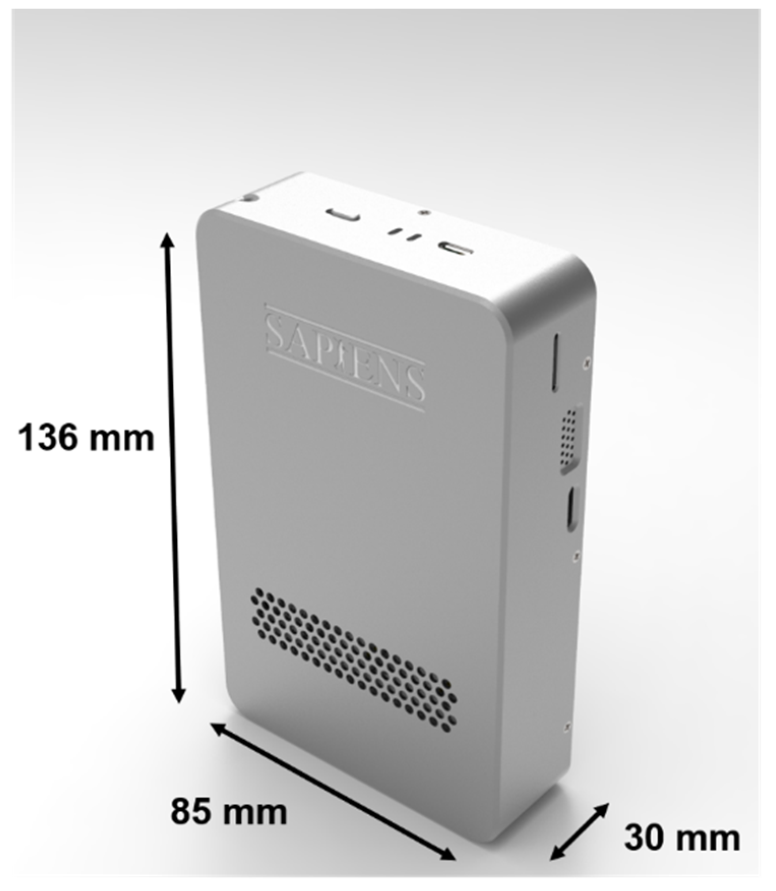
2.1. Description of the Personal Exposure Kit (PEK)
2.2. Laboratory Tests
2.2.1. Laboratory-Based Testing Protocols
2.2.2. Signal Linearity Test
2.2.3. Effects of Environmental Factors on Sensor Baseline
2.2.4. Sensor Response to Transient Pollutant Variation
2.2.5. Sensor Response to Transient Variation of Temperature and Humidity
2.3. Field Performance
2.3.1. Performance after Sensor Relocation
- Laboratory calibration—to assess suitability for field use, a laboratory calibrated PEK was deployed at reference sites to evaluate the robustness of the calibration with respect to accuracy and precision.
- Field co-location calibration—to quantify sensor changes among different environments, calibration took place via co-location at the TKO site and was subsequently validated via co-location at the other two sites for three days.
2.3.2. Performance in Dynamic and Changing Microenvironments
2.4. Data Analysis
3. Results and Discussion
3.1. Laboratory Tests
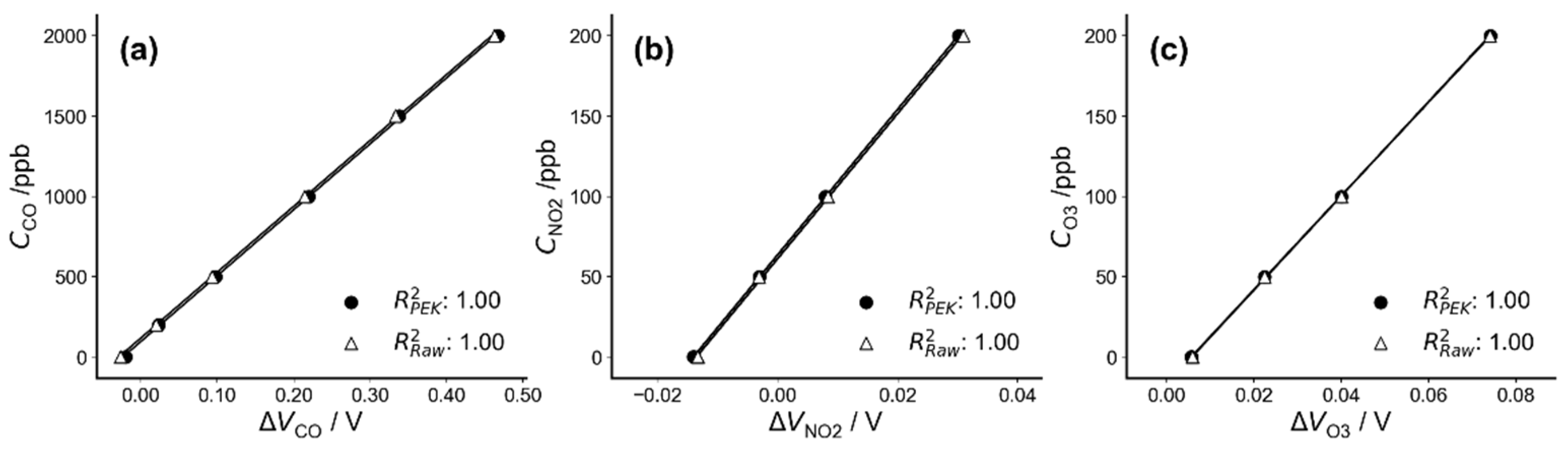
3.1.1. Signal Linearity
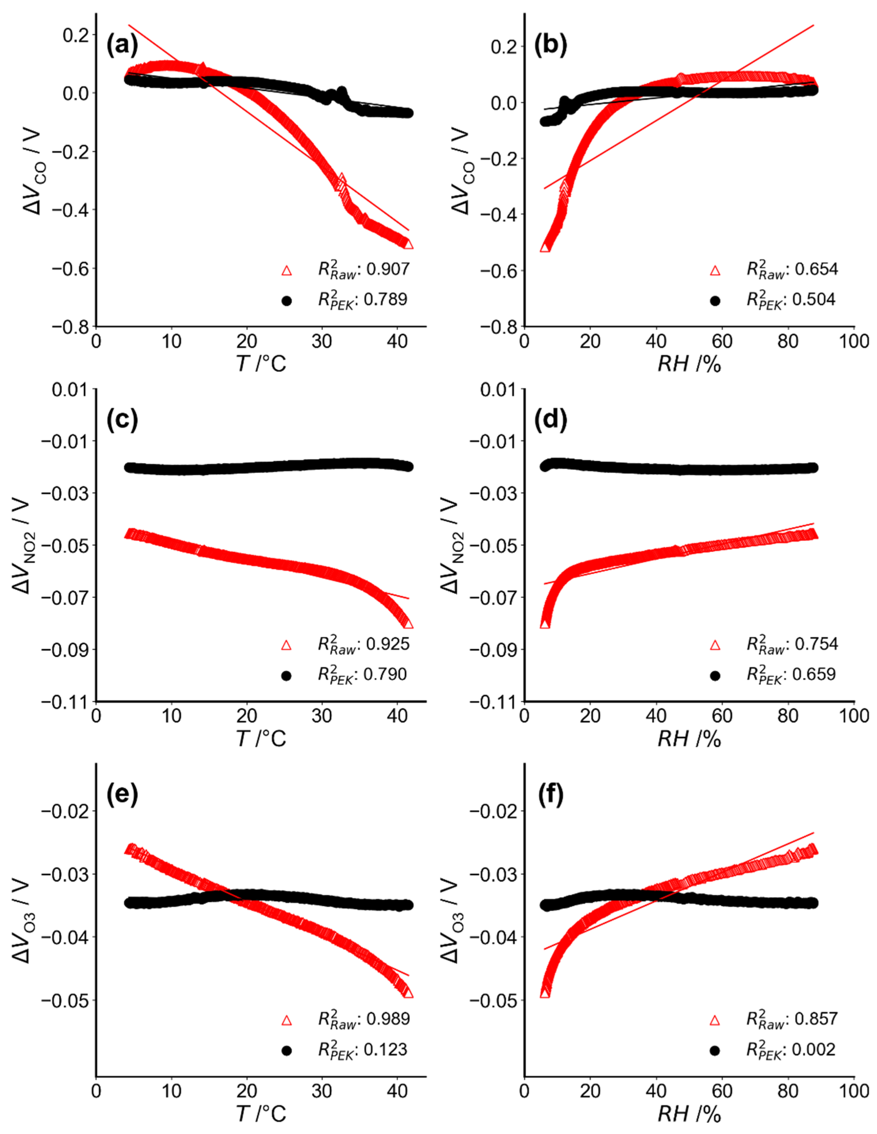
3.1.2. Analysis of Environmental Effects on Sensor Baseline
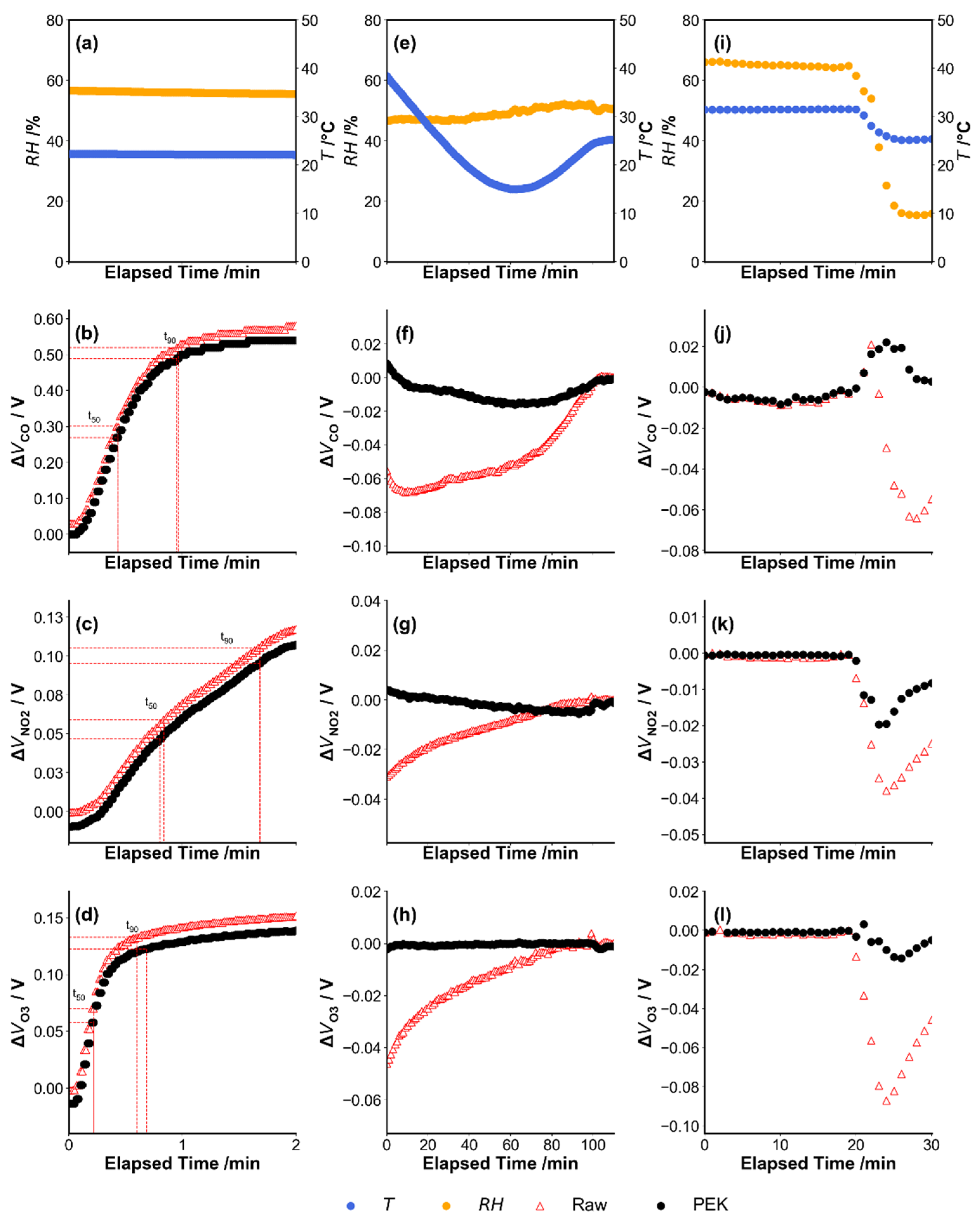
3.1.3. Response to Concentration and Simulated Ambient Conditions
3.2. Field Test Validation
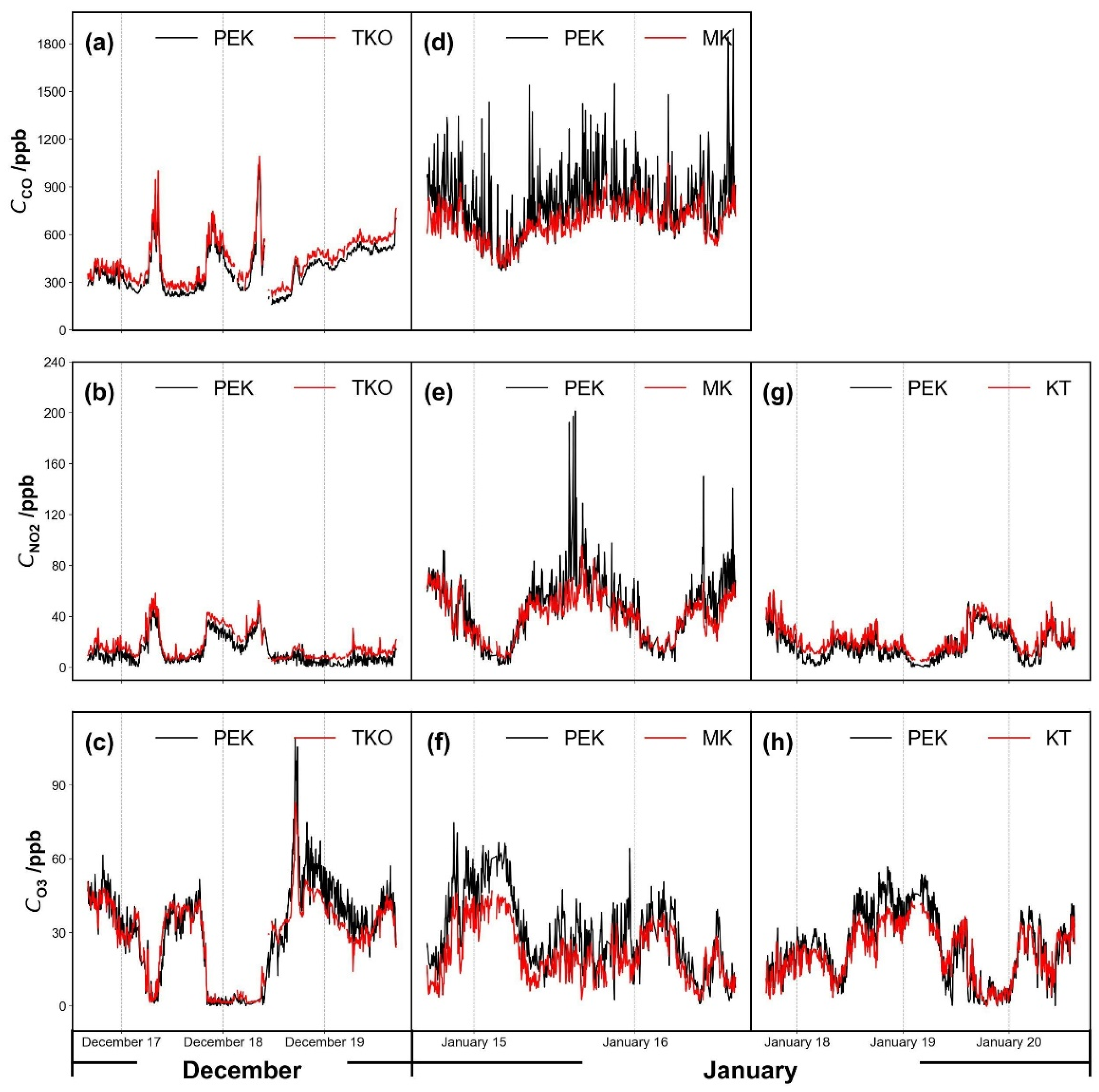
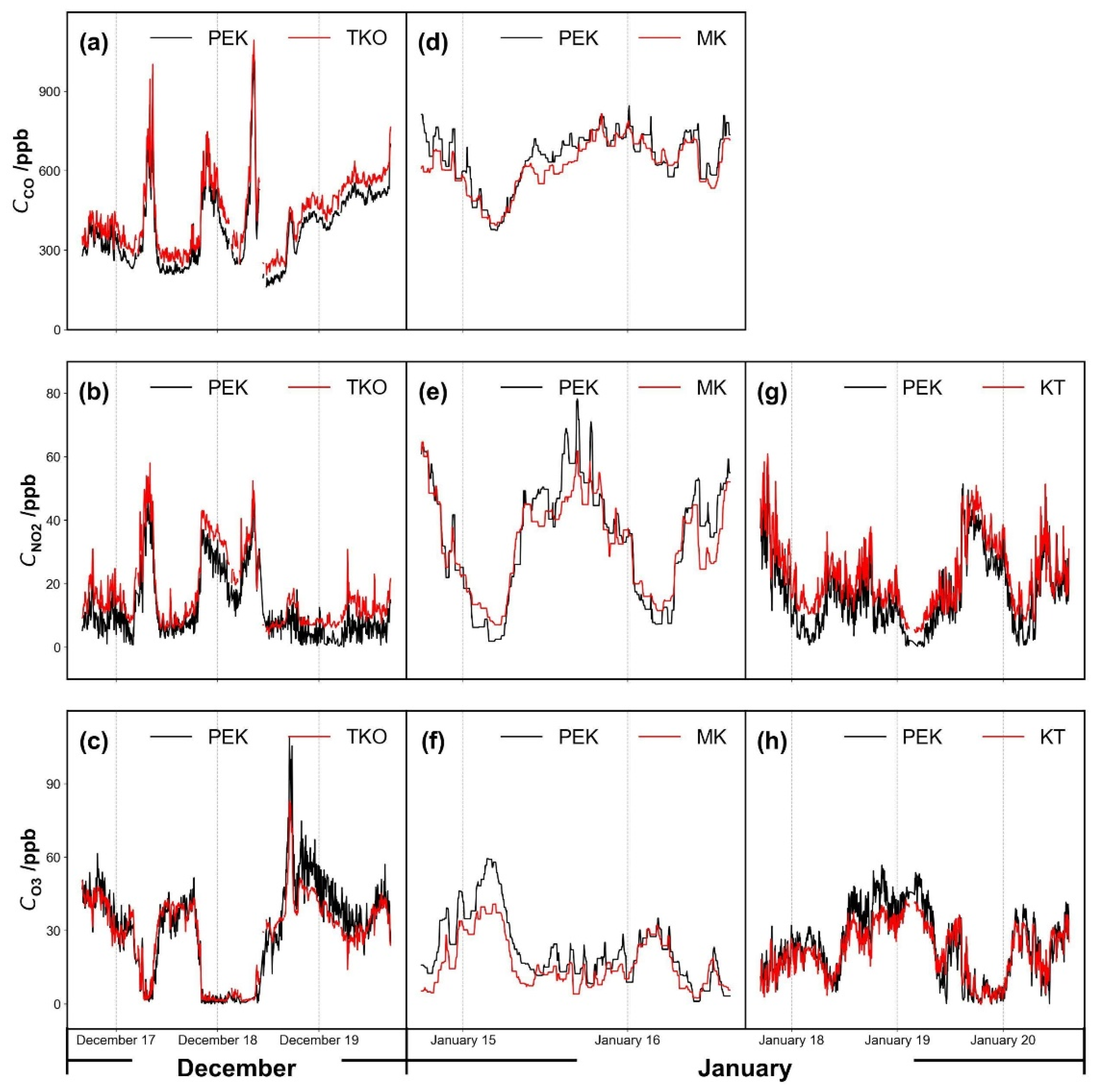
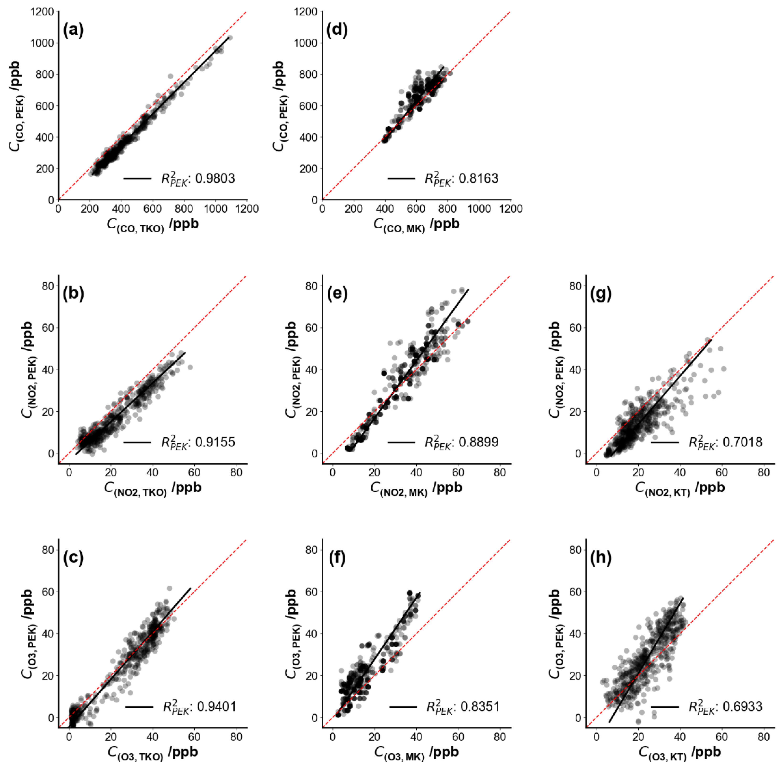
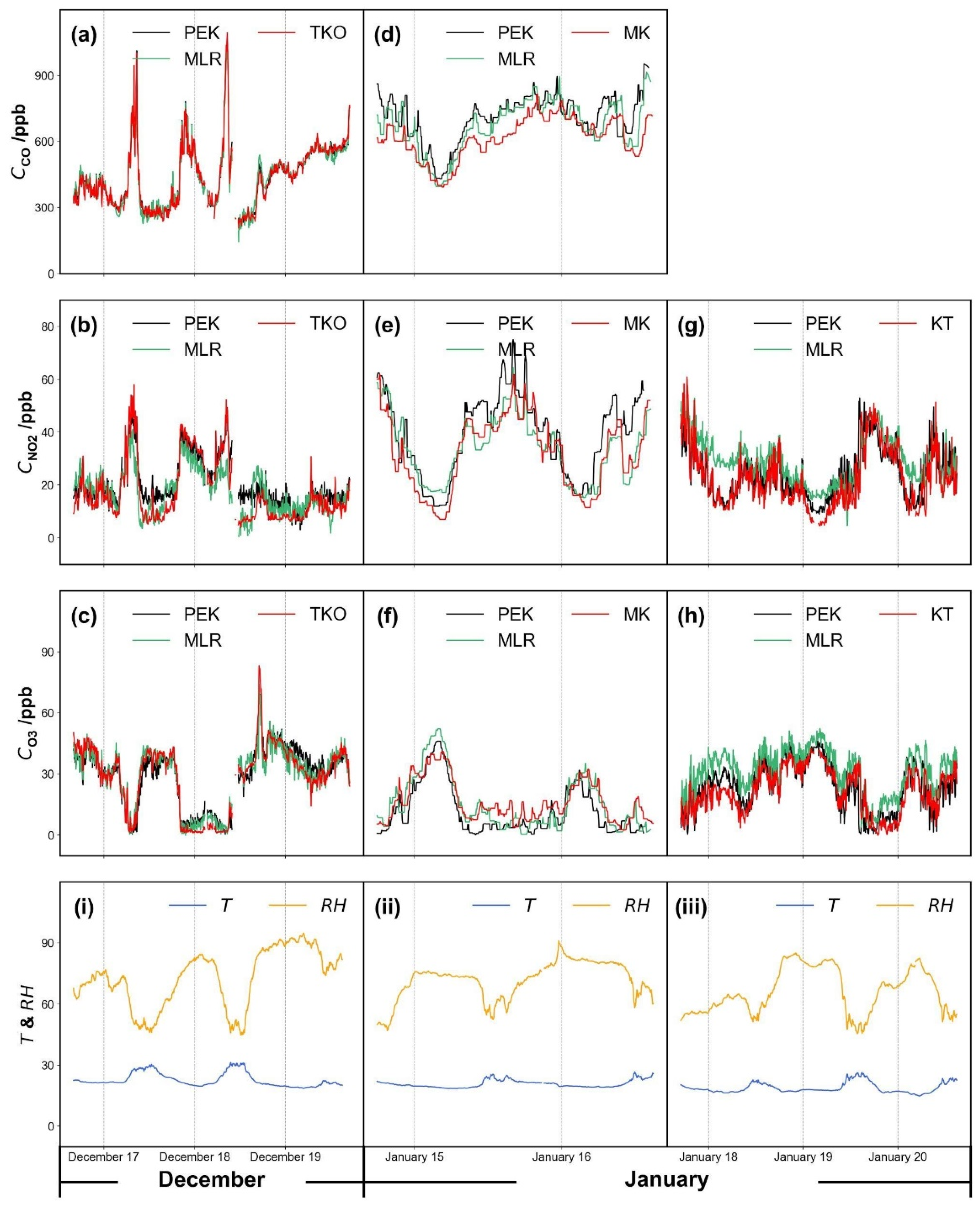
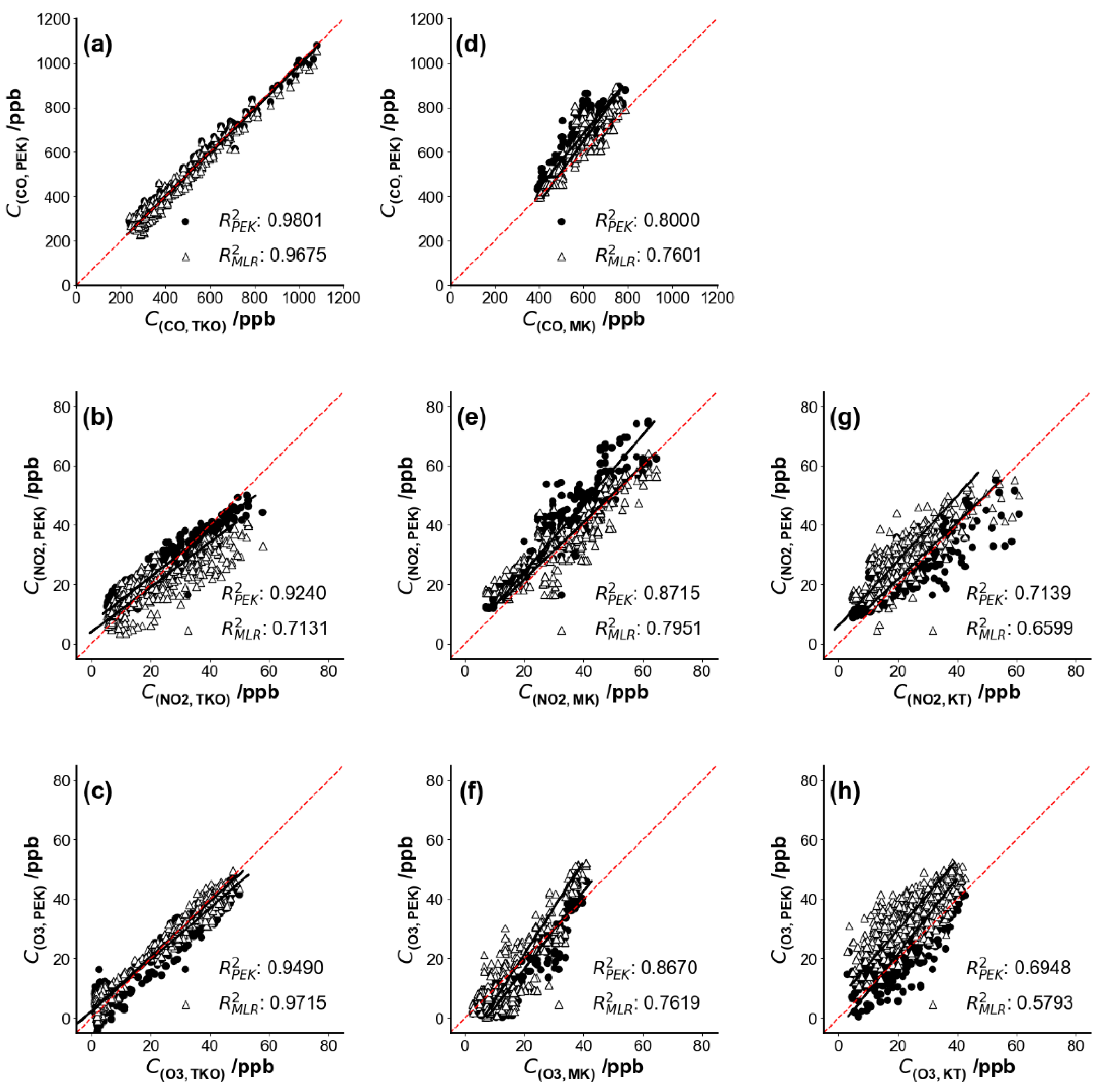
3.2.1. Applicability of Laboratory Calibration to Field Measurements
3.2.2. Sensor Change among Different Sites
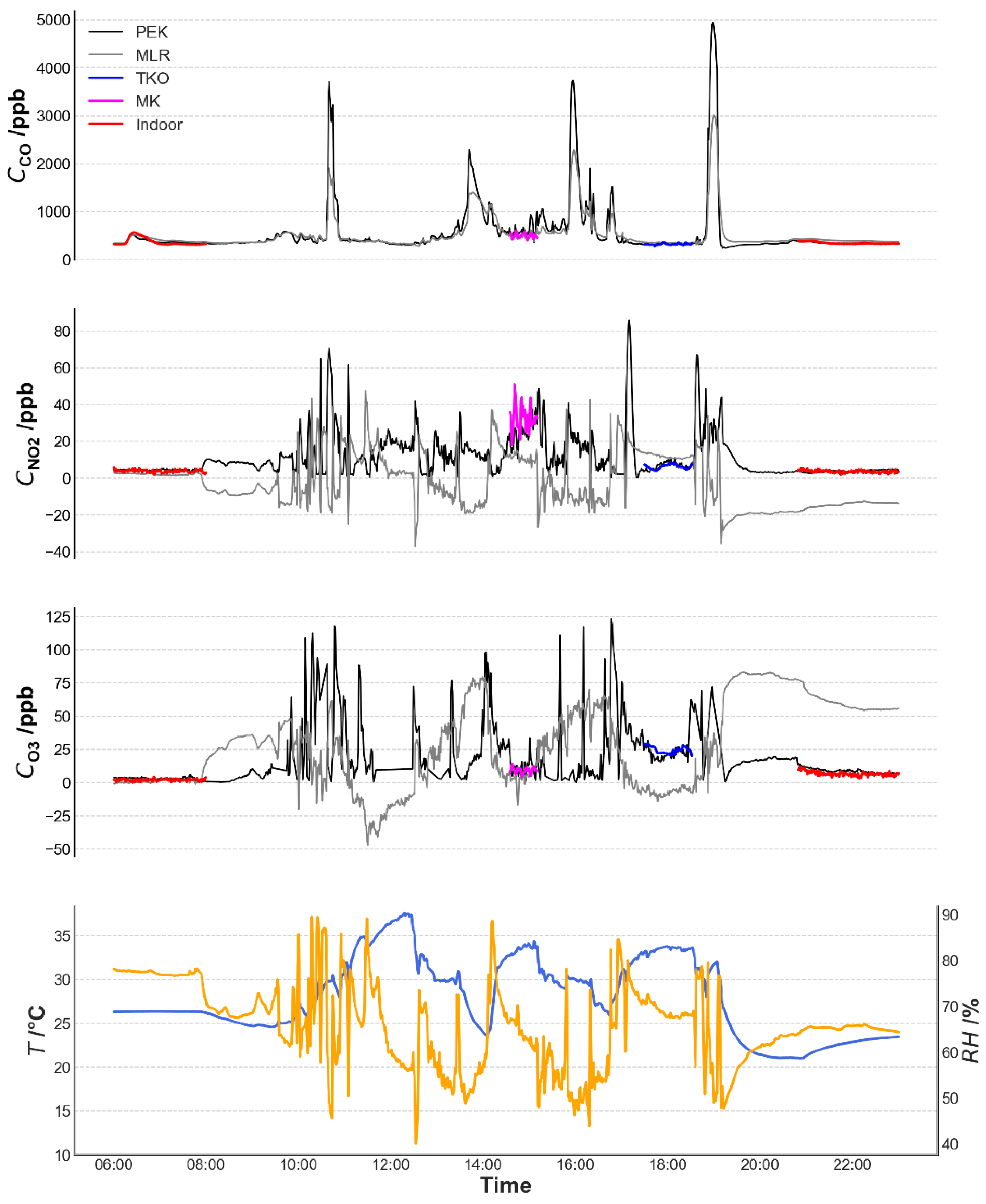
3.2.3. PEK Output during a Simulated Personal Exposure Assessment
4. Conclusions and Future Work
Author Contributions
Funding
Institutional Review Board Statement
Informed Consent Statement
Data Availability Statement
Acknowledgments
Conflicts of Interest
References
- Jantunen, E. A summary of methods applied to tool condition monitoring in drilling. Int. J. Mach. Tools Manuf. 2002, 42, 997–1010. [Google Scholar] [CrossRef]
- Monn, C. Exposure assessment of air pollutants: A review on spatial heterogeneity and indoor/outdoor/personal exposure to suspended particulate matter, nitrogen dioxide and ozone. Atmos. Environ. 2001, 35, 1–32. [Google Scholar] [CrossRef]
- Sexton, M.; Hebel, J.R. A clinical trial of change in maternal smoking and its effect on birth weight. JAMA 1984, 251, 911–915. [Google Scholar] [CrossRef] [PubMed]
- World Health Organization Ambient air pollution: A global assessment of exposure and burden of disease. Clean Air J. 2016, 26. [CrossRef]
- Kelly, F.J.; Fussell, J.C. Air pollution and public health: Emerging hazards and improved understanding of risk. Environ. Geochem. Heal. 2015, 37, 631–649. [Google Scholar] [CrossRef] [Green Version]
- Beeson, W.L.; E Abbey, D.; Knutsen, S.F. Long-term concentrations of ambient air pollutants and incident lung cancer in California adults: Results from the AHSMOG study.Adventist Health Study on Smog. Environ. Heal. Perspect. 1998, 106, 813–823. [Google Scholar] [CrossRef] [PubMed] [Green Version]
- Dockery, D.W.; Pope, C.A. Acute respiratory effects of particulate air pollution. Annu. Rev. Public Health 1994, 15, 107–132. [Google Scholar] [CrossRef]
- Katsouyanni, K.; Touloumi, G.; Spix, C.; Schwartz, J.; Balducci, F.; Medina, S.; Rossi, G.; Wojtyniak, B.; Sunyer, J.; Bacharova, L.; et al. Short term effects of ambient sulphur dioxide and particulate matter on mortality in 12 European cities: Results from time series data from the APHEA project. BMJ 1997, 314, 1658. [Google Scholar] [CrossRef] [Green Version]
- Baron, R.; Saffell, J. Amperometric Gas Sensors as a Low Cost Emerging Technology Platform for Air Quality Monitoring Applications: A Review. ACS Sens. 2017, 2, 1553–1566. [Google Scholar] [CrossRef]
- Che, W.; Frey, H.C.; Fung, J.C.; Ning, Z.; Qu, H.; Lo, H.K.; Chen, L.; Wong, T.-W.; Wong, M.K.; Lee, O.C.; et al. PRAISE-HK: A personalized real-time air quality informatics system for citizen participation in exposure and health risk management. Sustain. Cities Soc. 2020, 54, 101986. [Google Scholar] [CrossRef]
- Mead, M.; Popoola, O.; Stewart, G.; Landshoff, P.; Calleja, M.; Hayes, M.; Baldovi, J.; McLeod, M.; Hodgson, T.; Dicks, J.; et al. The use of electrochemical sensors for monitoring urban air quality in low-cost, high-density networks. Atmos. Environ. 2013, 70, 186–203. [Google Scholar] [CrossRef] [Green Version]
- Pang, X.; Shaw, M.D.; Lewis, A.C.; Carpenter, L.J.; Batchellier, T. Electrochemical ozone sensors: A miniaturised alternative for ozone measurements in laboratory experiments and air-quality monitoring. Sens. Actuators B Chem. 2017, 240, 829–837. [Google Scholar] [CrossRef] [Green Version]
- Pang, X.; Shaw, M.D.; Gillot, S.; Lewis, A.C. The impacts of water vapour and co-pollutants on the performance of electrochemical gas sensors used for air quality monitoring. Sens. Actuators B Chem. 2018, 266, 674–684. [Google Scholar] [CrossRef]
- Wei, P.; Ning, Z.; Ye, S.; Sun, L.; Yang, F.; Wong, K.C.; Westerdahl, D.; Louie, P.K.K. Impact Analysis of Temperature and Humidity Conditions on Electrochemical Sensor Response in Ambient Air Quality Monitoring. Sensors 2018, 18, 59. [Google Scholar] [CrossRef] [PubMed] [Green Version]
- Spinelle, L.; Gerboles, M.; Villani, M.G.; Aleixandre, M.; Bonavitacola, F. Field calibration of a cluster of low-cost commercially available sensors for air quality monitoring. Part B: NO, CO and CO2. Sens. Actuators B Chem. 2017, 238, 706–715. [Google Scholar] [CrossRef]
- Topalovic, D.; Davidovic, M.; Jovanović, M.; Bartonova, A.; Ristovski, Z.; Jovašević-Stojanović, M. In search of an optimal in-field calibration method of low-cost gas sensors for ambient air pollutants: Comparison of linear, multilinear and artificial neural network approaches. Atmos. Environ. 2019, 213, 640–658. [Google Scholar] [CrossRef]
- Popoola, O.; Stewart, G.; Mead, I.; Jones, R. Development of a baseline-temperature correction methodology for electrochemical sensors and its implications for long-term stability. Atmos. Environ 2017, 147, 330–343. [Google Scholar] [CrossRef] [Green Version]
- Sun, L.; Westerdahl, D.; Ning, Z. Development and Evaluation of a Novel and Cost-Effective Approach for Low-Cost NO2 Sensor Drift Correction. Sensors 2017, 17, 1916. [Google Scholar] [CrossRef]
- Sohn, J.H.; Atzeni, M.; Zeller, L.; Pioggia, G. Characterisation of humidity dependence of a metal oxide semiconductor sensor array using partial least squares. Sens. Actuators B Chem. 2008, 131, 230–235. [Google Scholar] [CrossRef]
- Wang, Y.; Li, J.; Jing, H.; Zhang, Q.; Jiang, J.; Biswas, P. Laboratory Evaluation and Calibration of Three Low-Cost Particle Sensors for Particulate Matter Measurement. Aerosol Sci. Technol. 2015, 49, 1063–1077. [Google Scholar] [CrossRef]
- Mijling, B.; Jiang, Q.; De Jonge, D.; Bocconi, S. Field calibration of electrochemical NO2 sensors in a citizen science context. Atmos. Meas. Tech. 2018, 11, 1297–1312. [Google Scholar] [CrossRef] [Green Version]
- Carslaw, N. A new detailed chemical model for indoor air pollution. Atmos. Environ. 2007, 41, 1164–1179. [Google Scholar] [CrossRef]
- Warburton, P.R.; Pagano, M.P.; Hoover, R.; Logman, A.M.; Crytzer, K.; Warburton, Y.J. Amperometric Gas Sensor Response Times. Anal. Chem. 1998, 70, 998–1006. [Google Scholar] [CrossRef] [PubMed]
- Piedrahita, R.; Xiang, Y.; Masson, N.; E Ortega, J.K.; Collier, A.; Jiang, Y.; Li, K.; Dick, R.P.; Lv, Q.; Hannigan, M.; et al. The next generation of low-cost personal air quality sensors for quantitative exposure monitoring. Atmos. Meas. Tech. 2014, 7, 3325–3336. [Google Scholar] [CrossRef] [Green Version]
- Malings, C.; Tanzer, R.; Hauryliuk, A.; Kumar, S.P.N.; Zimmerman, N.; Kara, L.B.; Presto, A.A.; Subramanian, R. Development of a general calibration model and long-term performance evaluation of low-cost sensors for air pollutant gas monitoring. Atmos. Meas. Tech. 2019, 12, 903–920. [Google Scholar] [CrossRef] [Green Version]
- Spinelle, L.; Gerboles, M.; Villani, M.G.; Aleixandre, M.; Bonavitacola, F. Calibration of a cluster of low-cost sensors for the measurement of air pollution in ambient air. In Proceedings of the IEEE SENSORS 2014, Valencia, Spain, 2–5 November 2014; pp. 21–24. [Google Scholar]
- McKinney, W. Python for Data Analysis: Data Wrangling with Pandas, NumPy, and IPython; O’Reilly Media: Newton, MA, USA, 2012. [Google Scholar]
- Brantley, H.L.; Hagler, G.S.W.; Kimbrough, E.S.; Williams, R.W.; Mukerjee, S.; Neas, L.M. Mobile air monitoring data-processing strategies and effects on spatial air pollution trends. Atmos. Meas. Tech. 2014, 7, 2169–2183. [Google Scholar] [CrossRef] [Green Version]
- Shairsingh, K.K.; Jeong, C.-H.; Wang, J.M.; Evans, G.J. Characterizing the spatial variability of local and background concentration signals for air pollution at the neighbourhood scale. Atmos. Environ. 2018, 183, 57–68. [Google Scholar] [CrossRef]


| P1 | P2 | MLR | |||||||
| CO | Validation | Calibration | Validation | Calibration | Validation | ||||
| ppb | TKO | MK | KT | TKO | MK | KT | TKO | MK | KT |
| MAE | 55.29 | 42.34 | - | 16.45 | 85.48 | - | 22.58 | 53.56 | - |
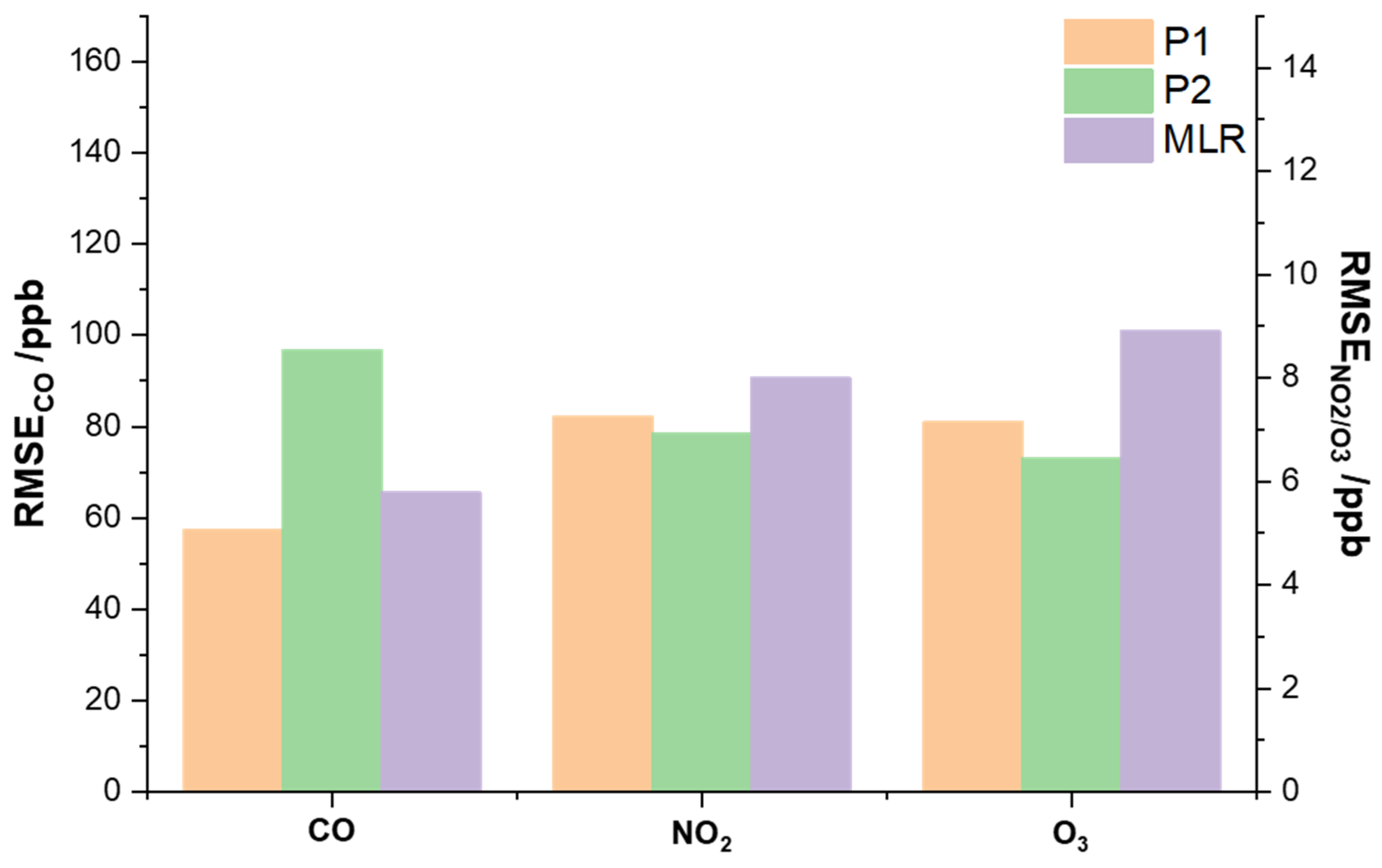
| RMSE | 58.88 | 55.93 | - | 21.66 | 96.74 | - | 28.07 | 65.51 | - |
| R2 | 0.98 | 0.81 | - | 0.98 | 0.80 | - | 0.98 | 0.88 | - |
| P1 | P2 | MLR | |||||||
| NO2 | Validation | Calibration | Validation | Calibration | Validation | ||||
| ppb | TKO | MK | KT | TKO | MK | KT | TKO | MK | KT |
| MAE | 5.44 | 5.63 | 6.93 | 4.16 | 6.76 | 4.26 | 5.83 | 5.16 | 8.59 |
| RMSE | 6.39 | 7.11 | 8.28 | 5.02 | 8.21 | 5.63 | 7.20 | 6.26 | 9.77 |
| R2 | 0.92 | 0.89 | 0.71 | 0.92 | 0.87 | 0.70 | 0.72 | 0.82 | 0.65 |
| P1 | P2 | MLR | |||||||
| O3 | Validation | Calibration | Validation | Calibration | Validation | ||||
| ppb | TKO | MK | KT | TKO | MK | KT | TKO | MK | KT |
| MAE | 3.68 | 6.75 | 6.68 | 3.77 | 5.35 | 5.28 | 2.62 | 4.59 | 10.56 |
| RMSE | 4.76 | 8.37 | 8.33 | 4.44 | 6.48 | 6.42 | 3.19 | 5.73 | 12.07 |
| R2 | 0.94 | 0.81 | 0.70 | 0.95 | 0.87 | 0.67 | 0.97 | 0.86 | 0.56 |
Publisher’s Note: MDPI stays neutral with regard to jurisdictional claims in published maps and institutional affiliations. |
© 2021 by the authors. Licensee MDPI, Basel, Switzerland. This article is an open access article distributed under the terms and conditions of the Creative Commons Attribution (CC BY) license (https://creativecommons.org/licenses/by/4.0/).
Share and Cite
Zong, H.; Brimblecombe, P.; Sun, L.; Wei, P.; Ho, K.-F.; Zhang, Q.; Cai, J.; Kan, H.; Chu, M.; Che, W.; et al. Reducing the Influence of Environmental Factors on Performance of a Diffusion-Based Personal Exposure Kit. Sensors 2021, 21, 4637. https://0-doi-org.brum.beds.ac.uk/10.3390/s21144637
Zong H, Brimblecombe P, Sun L, Wei P, Ho K-F, Zhang Q, Cai J, Kan H, Chu M, Che W, et al. Reducing the Influence of Environmental Factors on Performance of a Diffusion-Based Personal Exposure Kit. Sensors. 2021; 21(14):4637. https://0-doi-org.brum.beds.ac.uk/10.3390/s21144637
Chicago/Turabian StyleZong, Huixin, Peter Brimblecombe, Li Sun, Peng Wei, Kin-Fai Ho, Qingli Zhang, Jing Cai, Haidong Kan, Mengyuan Chu, Wenwei Che, and et al. 2021. "Reducing the Influence of Environmental Factors on Performance of a Diffusion-Based Personal Exposure Kit" Sensors 21, no. 14: 4637. https://0-doi-org.brum.beds.ac.uk/10.3390/s21144637