
Machine Learning-Based Estimation of Ground Reaction Forces and Knee Joint Kinetics from Inertial Sensors While Performing a Vertical Drop Jump


 , ,
, ,  ,
,  and
and
Abstract
:1. Introduction
2. Materials and Methods
2.1. Participants and Experimental Procedures
2.2. Experimental Setup
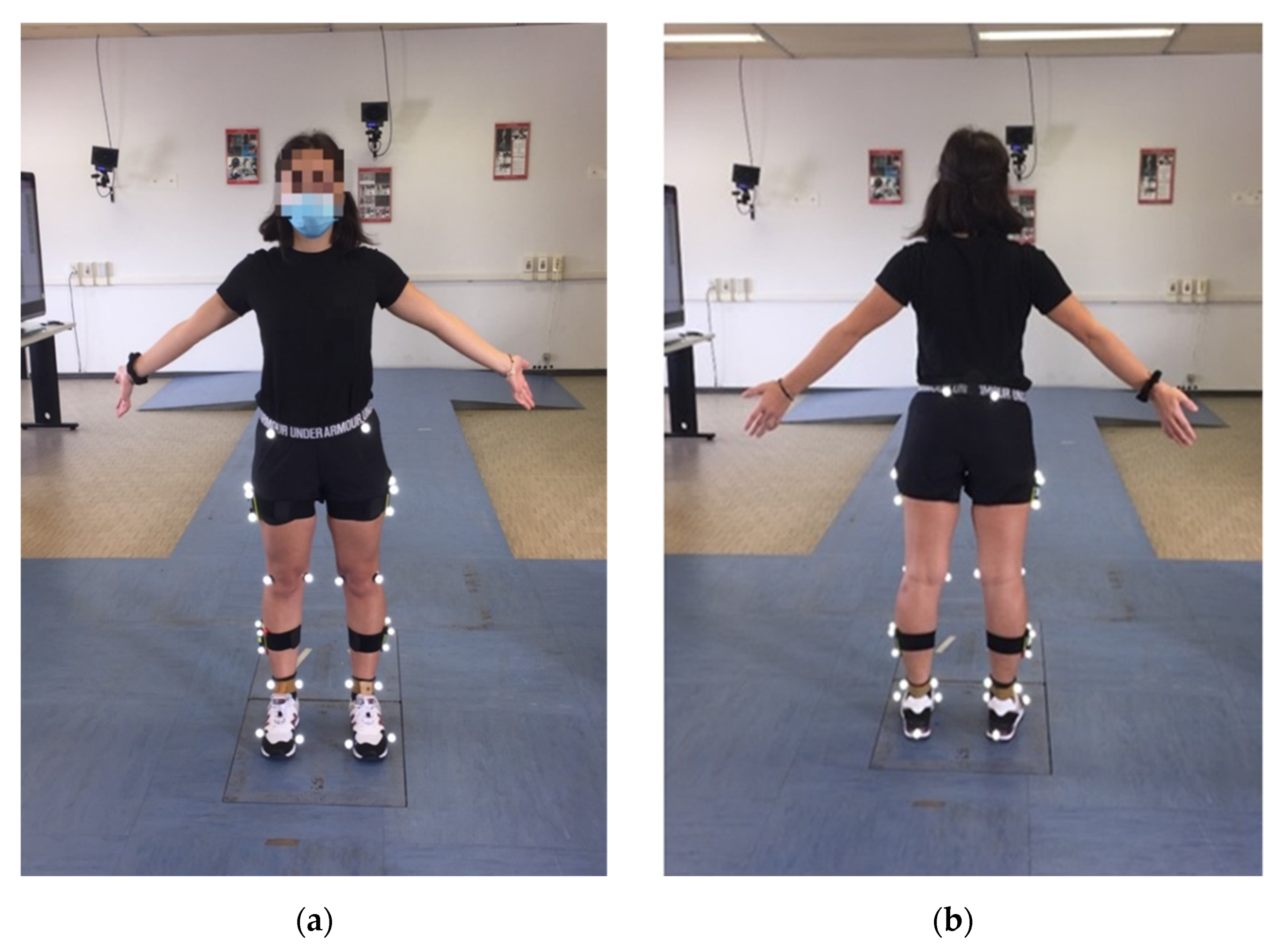
2.2.1. Marker Set
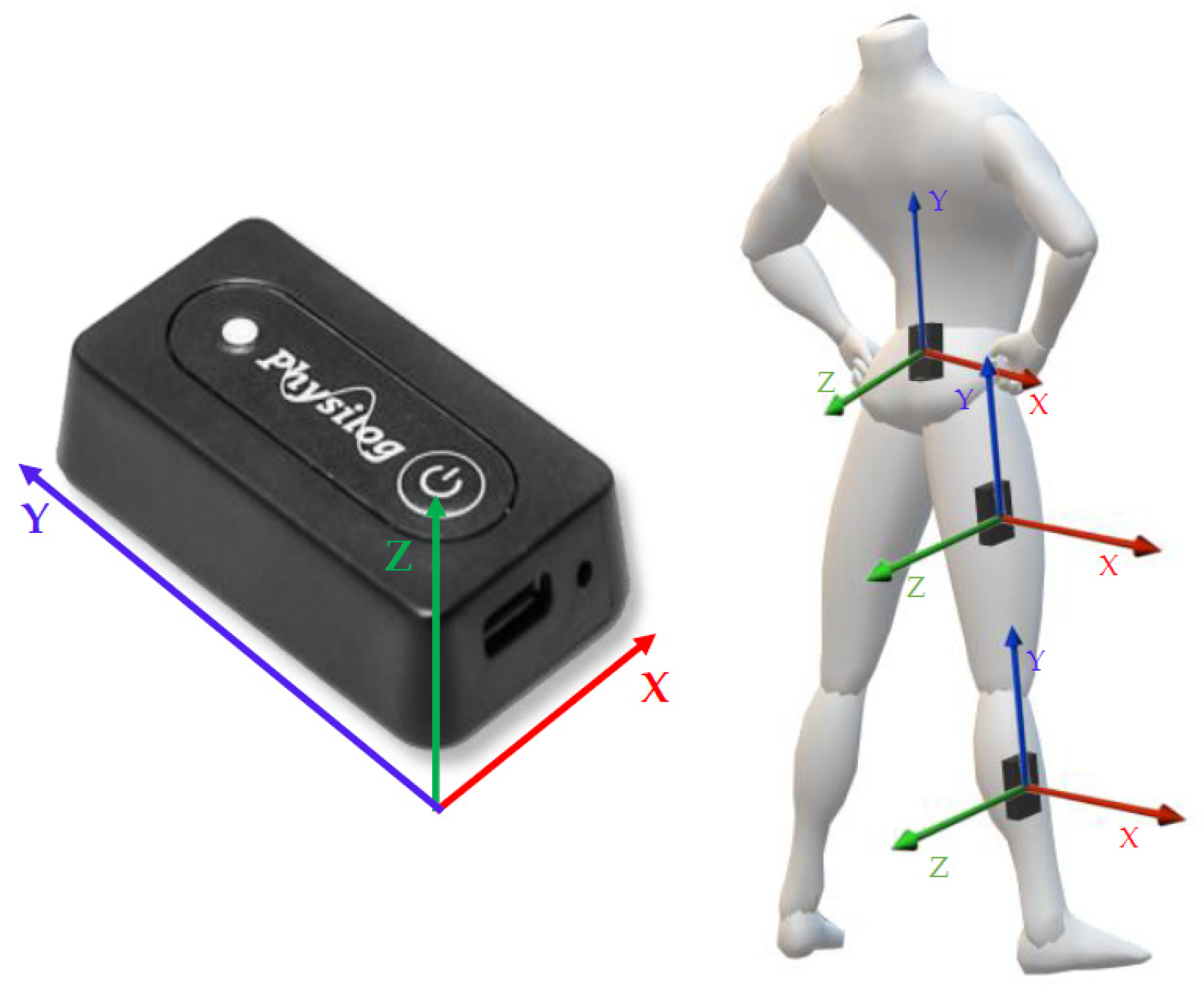
2.2.2. IMU Devices
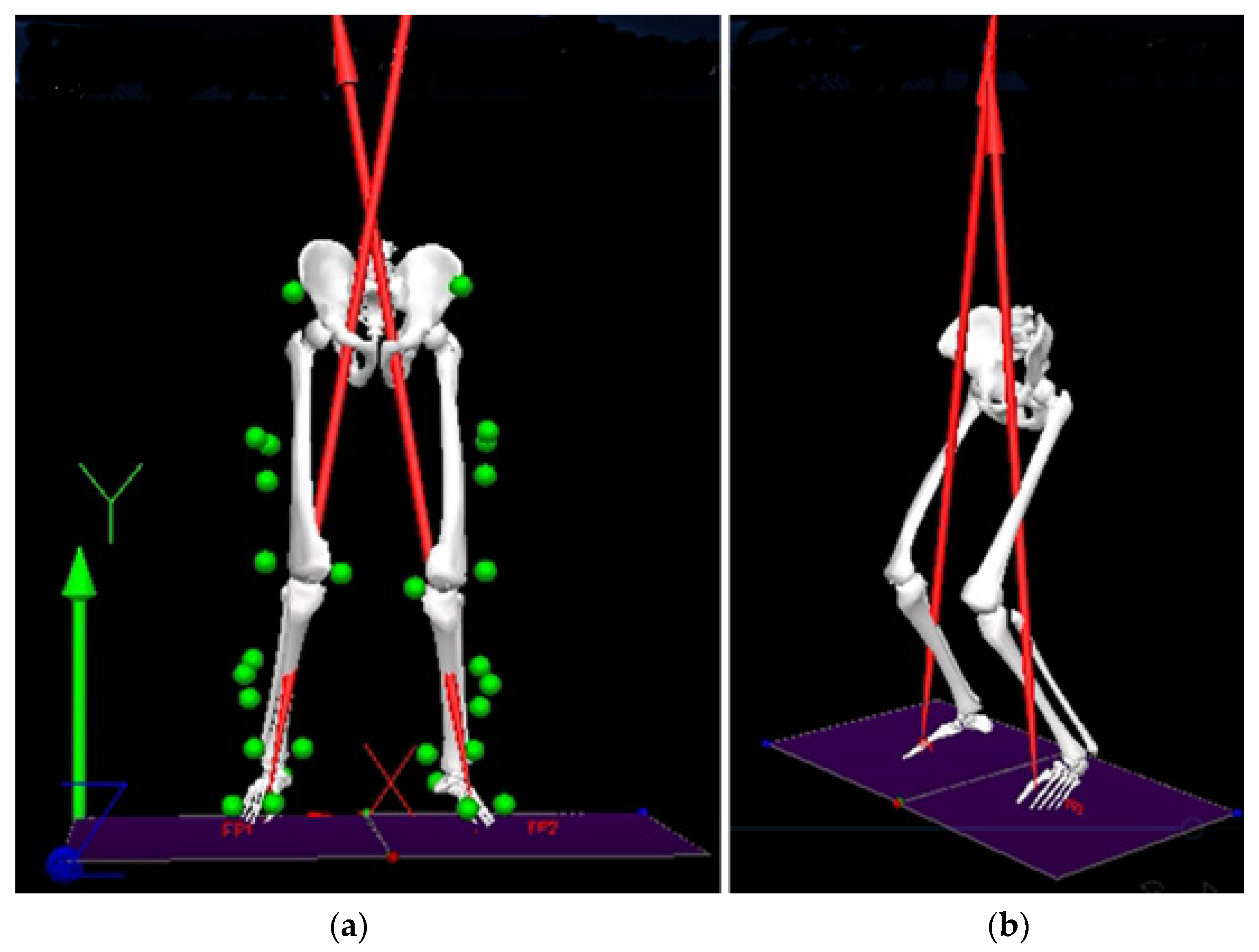
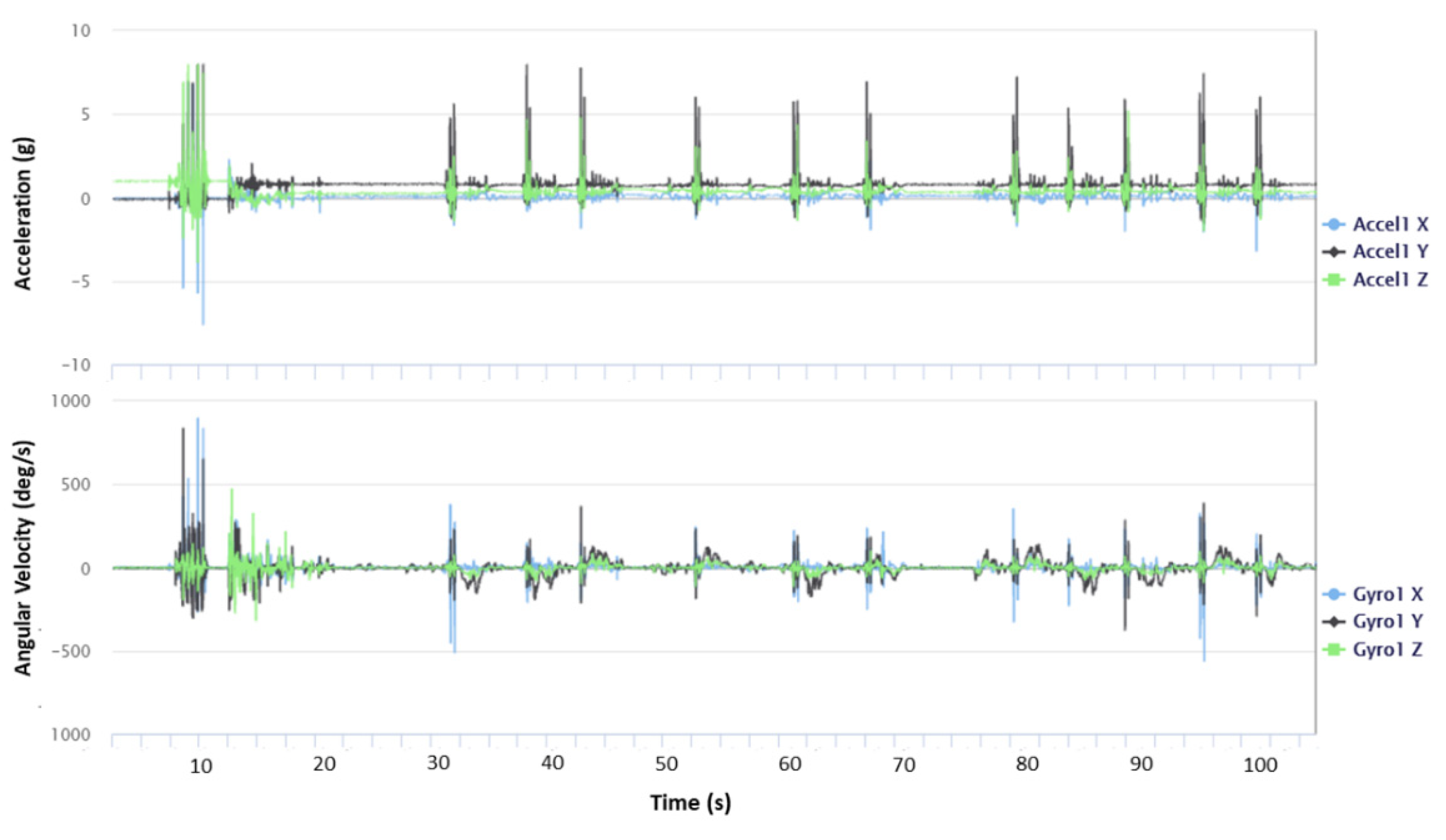
2.3. Data Analysis and Processing
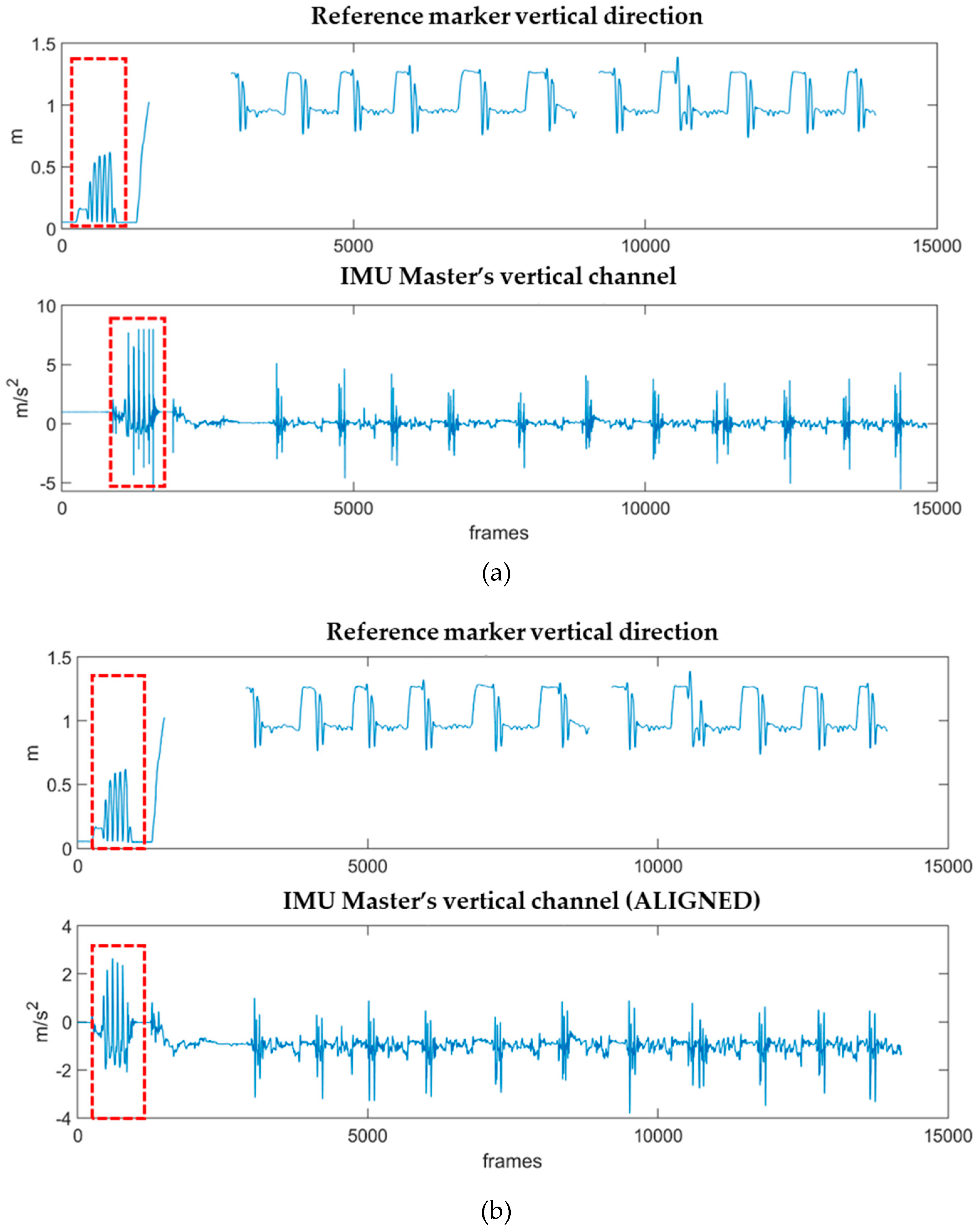
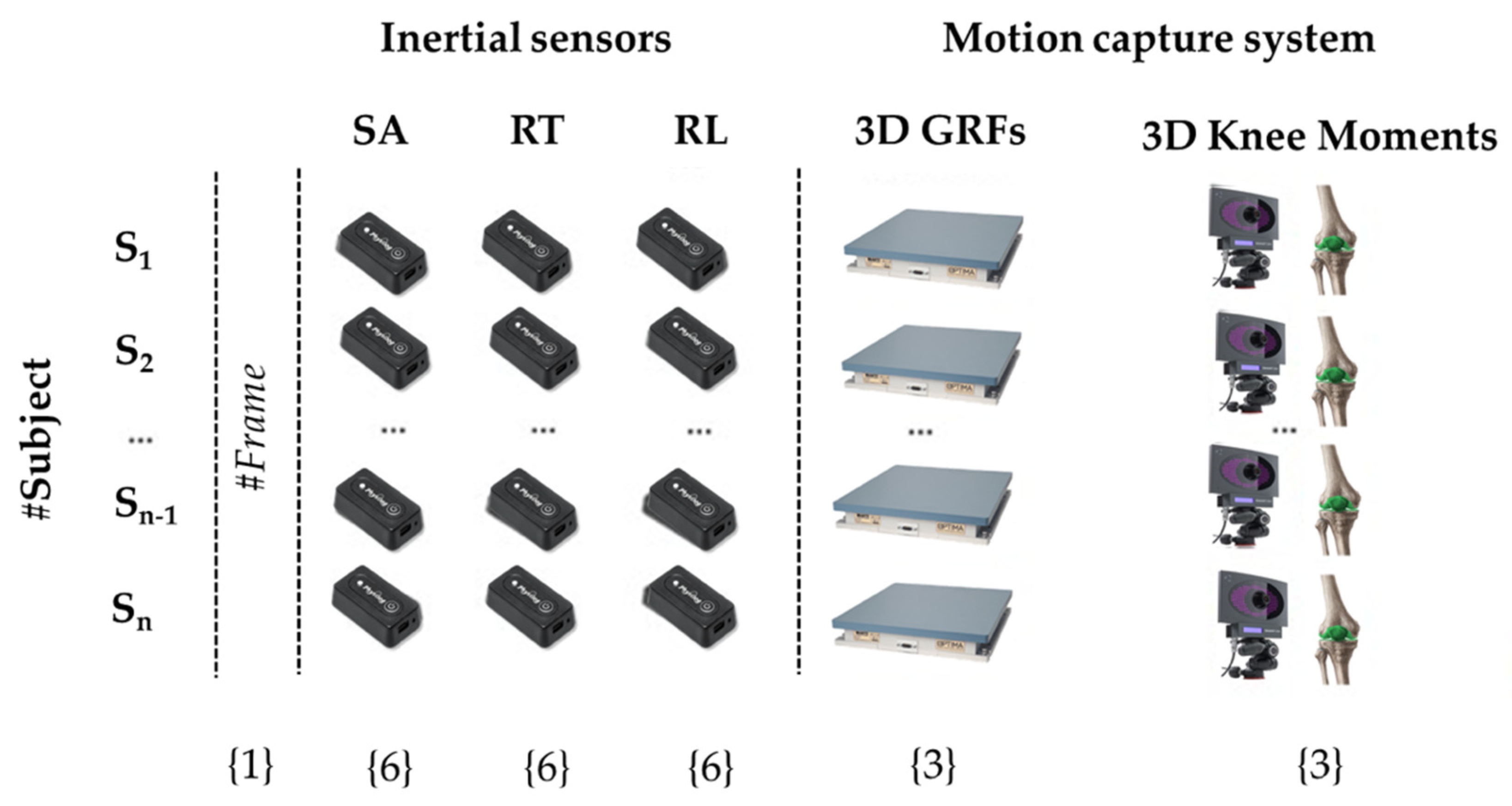
2.4. Data Synchronization and Dataset Structure
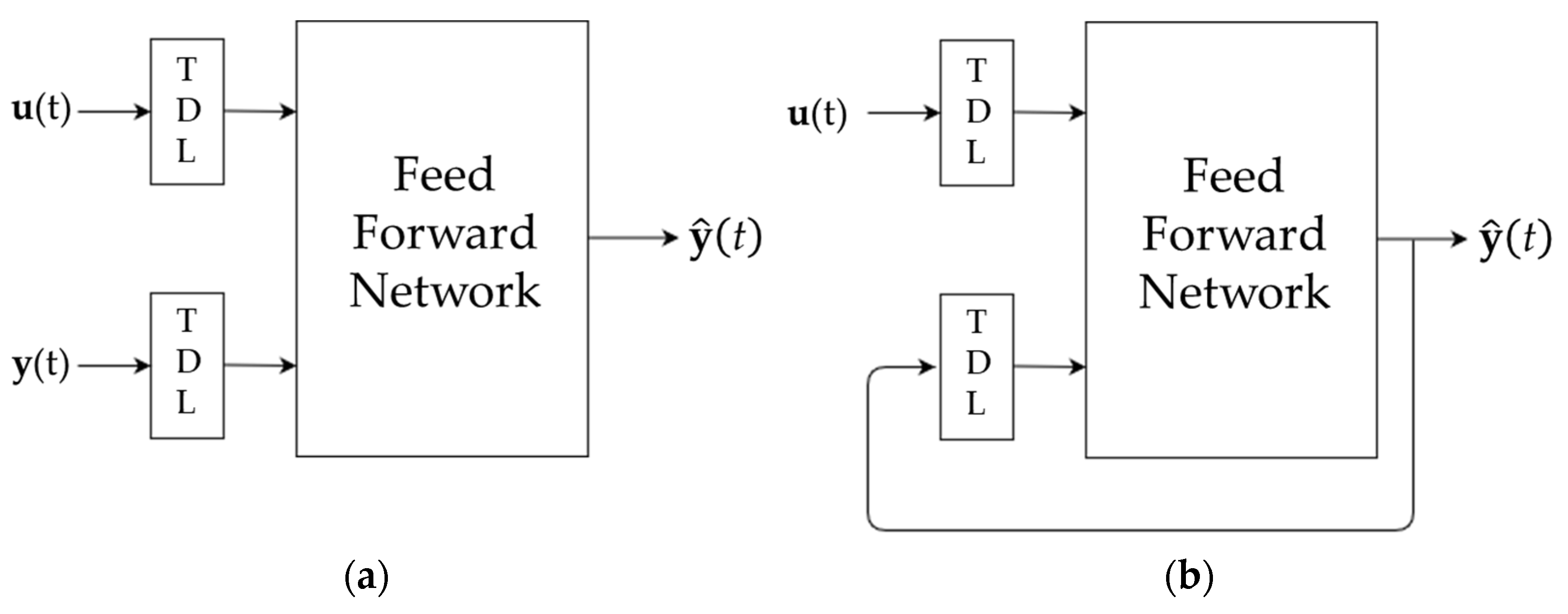
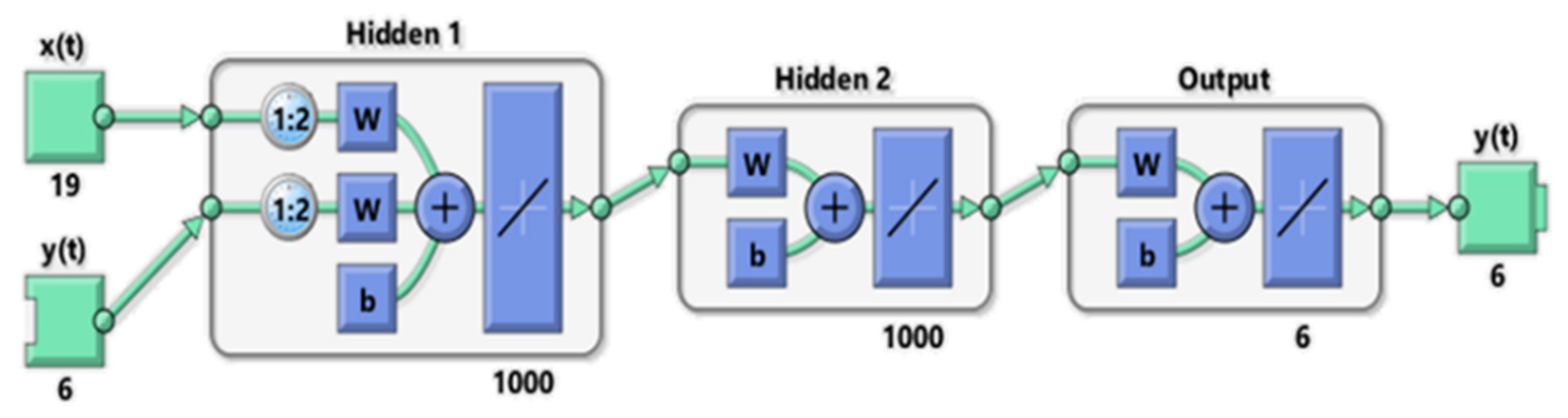
2.5. Neural Network Implementation
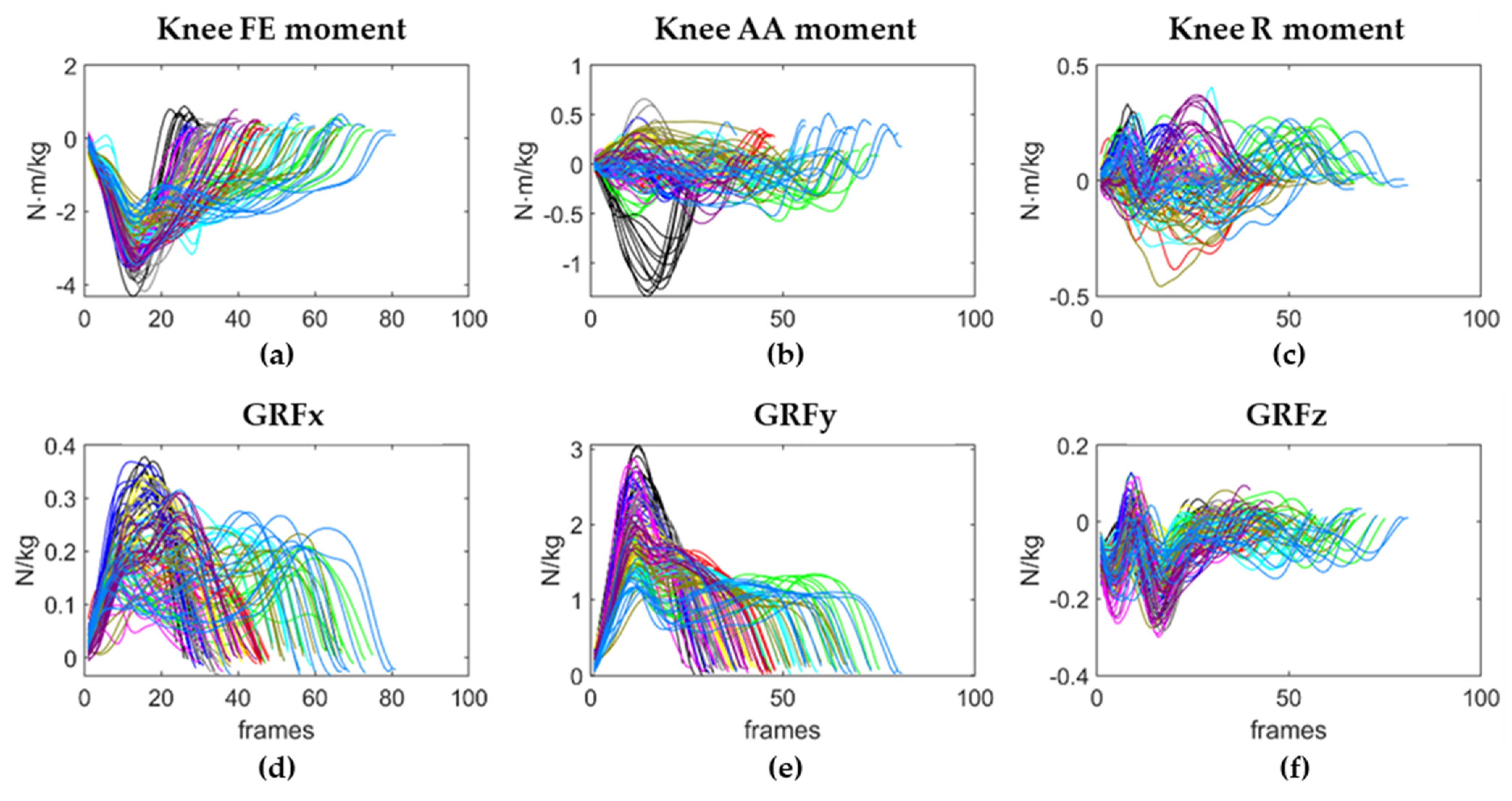
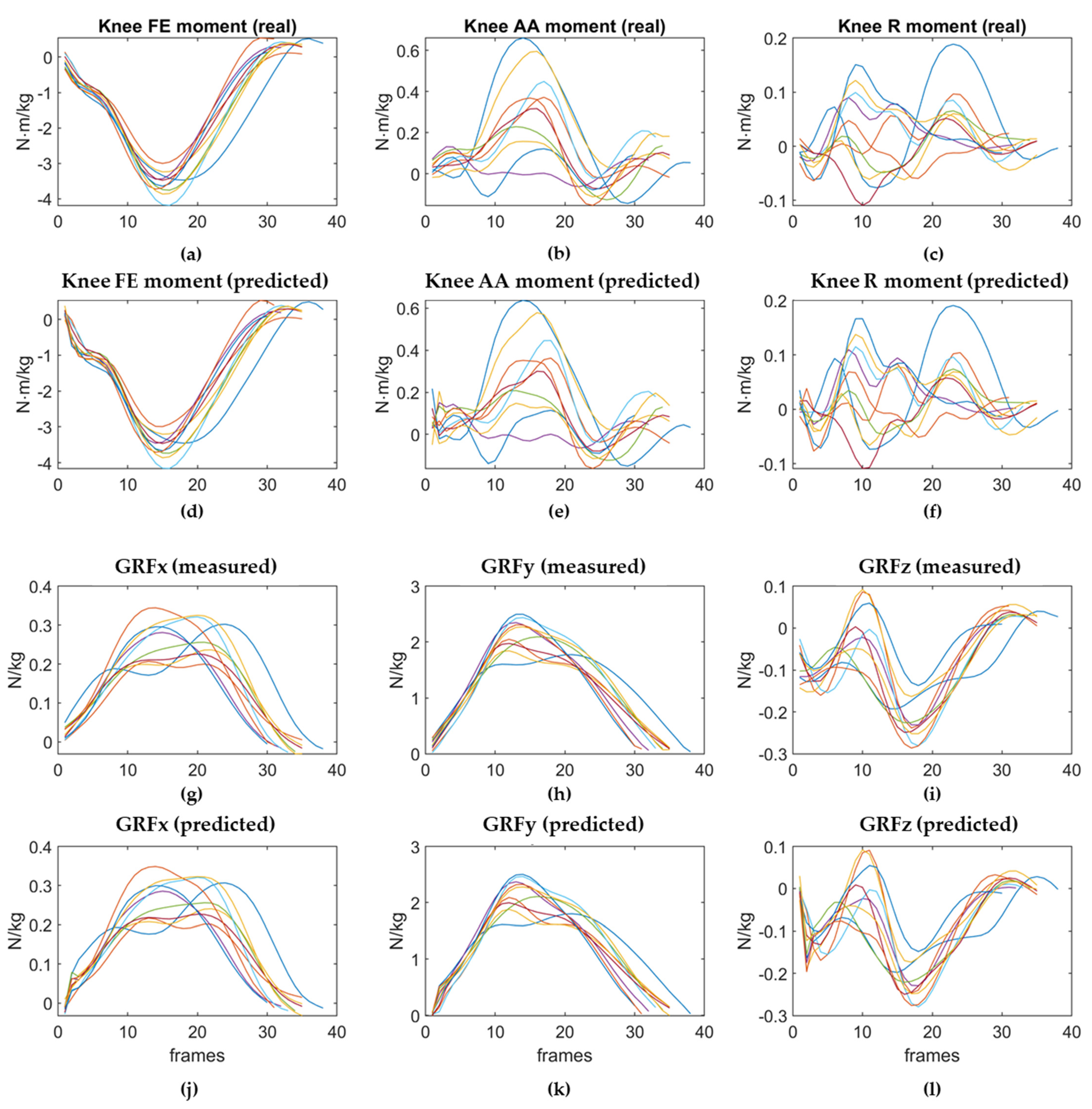
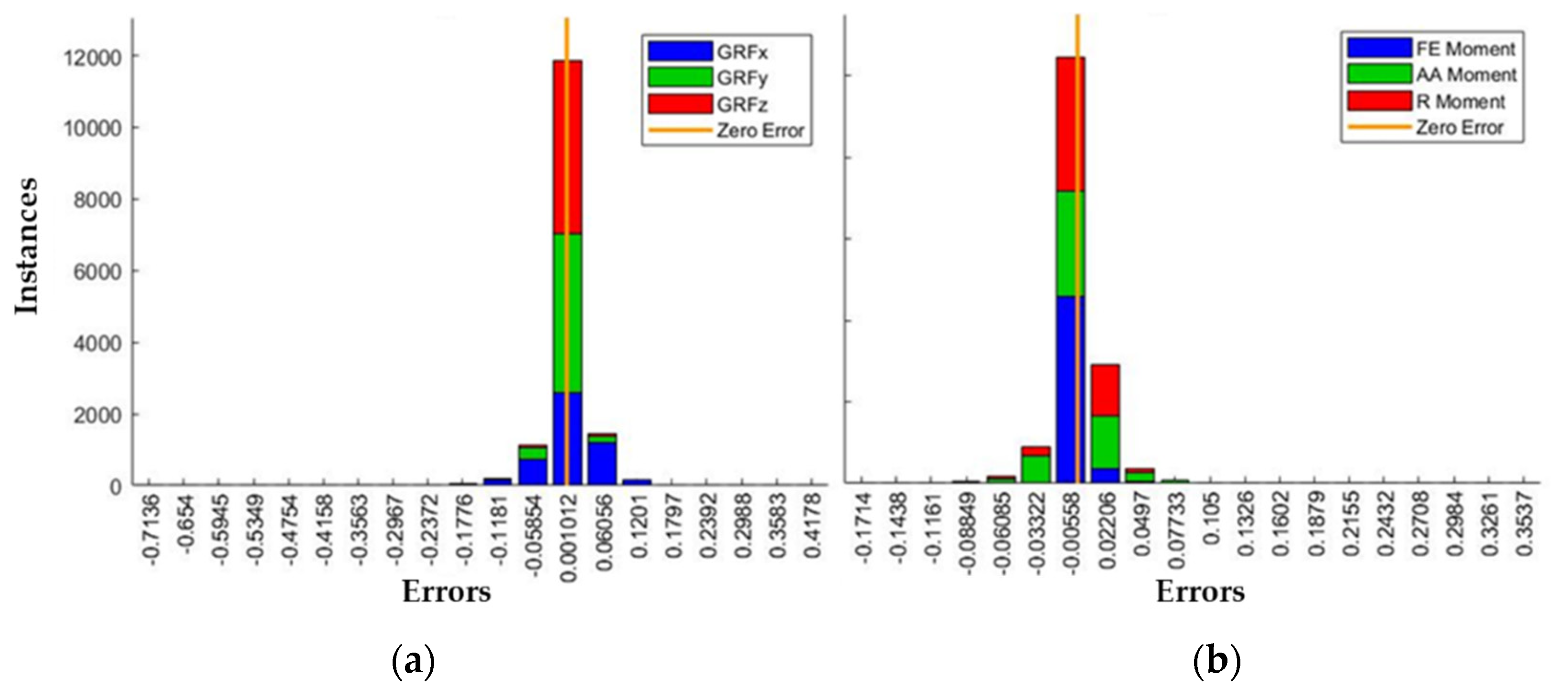
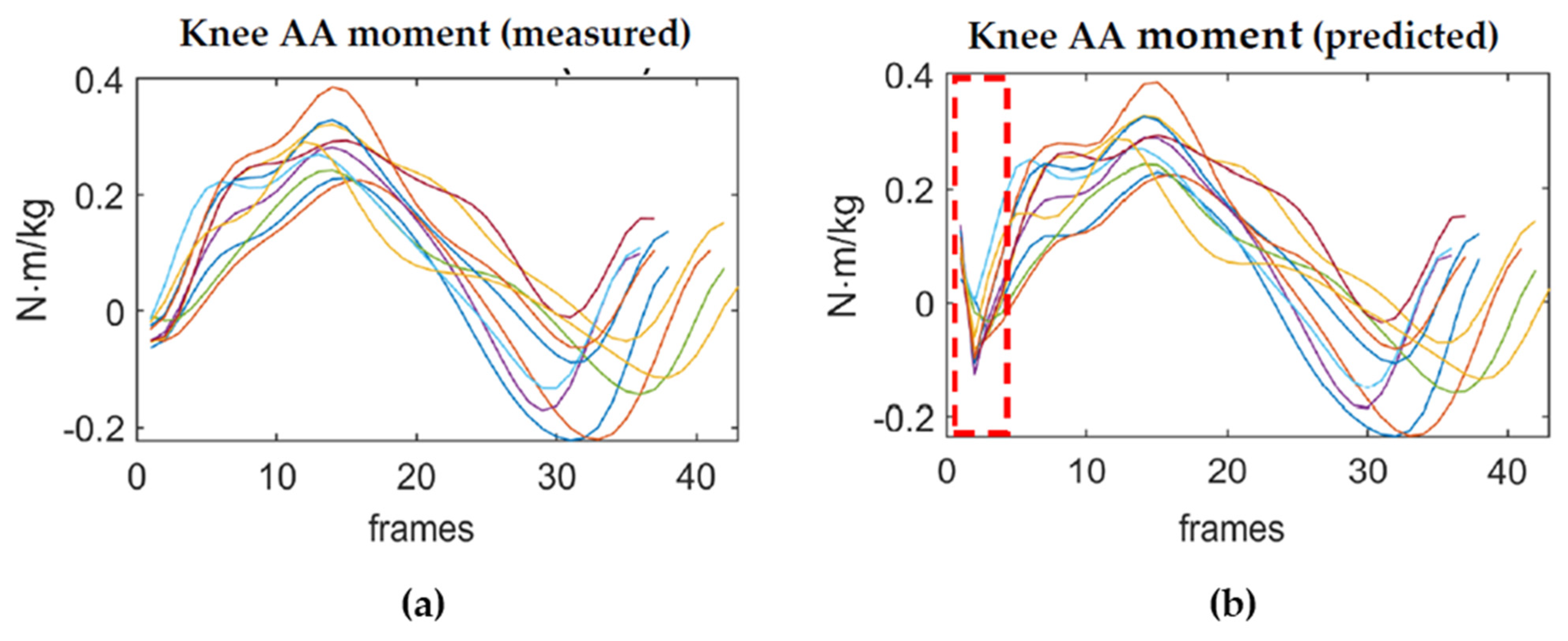
3. Results
4. Discussion
4.1. Novelty of the Study
4.2. Limitations
5. Conclusions
Author Contributions
Funding
Institutional Review Board Statement
Informed Consent Statement
Data Availability Statement
Conflicts of Interest
References
- Pedley, J.S.; Lloyd, R.S.; Read, P.; Moore, I.S.; Oliver, J.L. Drop jump: A technical model for scientific application. Strength Cond. J. 2017, 39, 36–44. [Google Scholar] [CrossRef]
- Eiras, A.E.; Ladeira, R.; Silva, P.A.; André, N.; Pereira, R.; Machado, M. Drop jump and muscle damage markers. Serb. J. Sport. Sci. 2009, 3, 81–84. [Google Scholar]
- Augustsson, S.R.; Tranberg, R.; Zügner, R.; Augustsson, J. Vertical drop jump landing depth influences knee kinematics in female recreational athletes. Phys. Ther. Sport 2018, 33, 133–138. [Google Scholar] [CrossRef] [PubMed]
- Chimera, N.J.; Warren, M. Use of clinical movement screening tests to predict injury in sport. World J. Orthop. 2016, 7, 202–217. [Google Scholar] [CrossRef] [PubMed]
- Mok, K.M.; Petushek, E.; Krosshaug, T. Reliability of knee biomechanics during a vertical drop jump in elite female athletes. Gait Posture 2016, 46, 173–178. [Google Scholar] [CrossRef] [PubMed] [Green Version]
- Kristianslund, E.; Krosshaug, T. Comparison of drop jumps and sport-specific sidestep cutting: Implications for anterior cruciate ligament injury risk screening. Am. J. Sports Med. 2013, 41, 684–688. [Google Scholar] [CrossRef] [PubMed]
- Smith, H.C.; Johnson, R.J.; Shultz, S.J.; Tourville, T.; Holterman, L.A.; Slauterbeck, J.; Pamela Vacek, M.; Beynnon, B.D. A Prospective Evaluation of the Landing Error Scoring System (LESS) as a Screening Tool for Anterior Cruciate Ligament Injury Risk. Am. J. Sports Med. 2012, 40, 521–526. [Google Scholar] [CrossRef] [PubMed]
- Cronström, A.; Creaby, M.W.; Ageberg, E. Do knee abduction kinematics and kinetics predict future anterior cruciate ligament injury risk? A systematic review and meta-analysis of prospective studies. BMC Musculoskelet. Disord. 2020, 21, 1–11. [Google Scholar] [CrossRef]
- Lucarno, S.; Zago, M.; Rossi, E.; Muratore, S.; Baroncini, G.; Alberti, G.; Gualtieri, D. Influence of age and sex on drop jump landing strategies in élite youth soccer players. Int. J. Sports Sci. Coach. 2020, 16, 344–351. [Google Scholar] [CrossRef]
- Hewett, T.E.; Myer, G.D.; Ford, K.R.; Paterno, M.V.; Quatman, C.E. Mechanisms, Prediction, and Prevention of ACL Injuries: Cut Risk With Three Sharpened and Validated Tools. J. Orthop. Res. 2016, 34, 1843–1855. [Google Scholar] [CrossRef] [PubMed] [Green Version]
- Hewett, T.E.; Myer, G.D.; Ford, K.R.; Heidt, R.S.; Colosimo, A.J.; McLean, S.G.; Van Den Bogert, A.J.; Paterno, M.V.; Succop, P. Biomechanical measures of neuromuscular control and valgus loading of the knee predict anterior cruciate ligament injury risk in female athletes: A prospective study. Am. J. Sports Med. 2005, 33, 492–501. [Google Scholar] [CrossRef] [Green Version]
- Mundt, M.; David, S.; Koeppe, A.; Bamer, F.; Markert, B.; Potthast, W. Intelligent prediction of kinetic parameters during cutting manoeuvres. Med. Biol. Eng. Comput. 2019, 57, 1833–1841. [Google Scholar] [CrossRef] [PubMed]
- Ekegren, C.L.; Miller, W.C.; Celebrin, R.G.; Eng, J.J.; MacIntyre, D.L. Reliability and validity of observational risk screening in evaluating dynamic knee valgus. J. Orthop. Sports Phys. Ther. 2009, 39, 665–674. [Google Scholar] [CrossRef] [PubMed] [Green Version]
- Fox, A.S.; Bonacci, J.; McLean, S.G.; Spittle, M.; Saunders, N. What is normal? Female lower limb kinematic profiles during athletic tasks used to examine anterior cruciate ligament injury risk: A systematic review. Sports Med. 2014, 44, 815–832. [Google Scholar] [CrossRef] [PubMed]
- Nilstad, A.; Krosshaug, T.; Mok, K.M.; Bahr, R.; Andersen, T.E. Association between anatomical characteristics, knee laxity, muscle strength, and peak knee valgus during vertical drop-jump landings. J. Orthop. Sports Phys. Ther. 2015, 45, 998–1005. [Google Scholar] [CrossRef] [PubMed]
- Dowling, A.V.; Favre, J.; Andriacchi, T.P. A wearable system to assess risk for anterior cruciate ligament injury during jump landing: Measurements of temporal events, jump height, and sagittal plane kinematics. J. Biomech. Eng. 2011, 133, 1–7. [Google Scholar] [CrossRef]
- Robert-Lachaine, X.; Mecheri, H.; Larue, C.; Plamondon, A. Validation of inertial measurement units with an optoelectronic system for whole-body motion analysis. Med. Biol. Eng. Comput. 2017, 55, 609–619. [Google Scholar] [CrossRef] [PubMed]
- Teufl, W.; Miezal, M.; Taetz, B.; Frohlichi, M.; Bleser, G. Validity of inertial sensor based 3D joint kinematics of static and dynamic sport and physiotherapy specific movements. PLoS ONE 2019, 14, e0213064. [Google Scholar] [CrossRef] [Green Version]
- Wang, L.; Cheng, L.; Zhao, G. Machine Learning for Human Motion Analysis: Theory and Practice; IGI Global: Hershey, PA, USA, 2009. [Google Scholar] [CrossRef] [Green Version]
- Seel, T.; Raisch, J.; Schauer, T. IMU-based joint angle measurement for gait analysis. Sensors 2014, 14, 6891–6909. [Google Scholar] [CrossRef] [PubMed] [Green Version]
- Schmidt, M.; Jaitner, T.; Nolte, K.; Rheinländer, C.; Wille, S.; Wehn, N. A wearable inertial sensor unit for jump diagnosis in multiple athletes. In Proceedings of the icSPORTS 2014—2nd International Congress on Sports Sciences Research and Technology Support, Rome, Italy, 24–26 October 2014; pp. 216–220. [Google Scholar] [CrossRef] [Green Version]
- Adesida, Y.; Papi, E.; McGregor, A.H. Exploring the role of wearable technology in sport kinematics and kinetics: A systematic review. Sensors 2019, 19, 1597. [Google Scholar] [CrossRef] [PubMed] [Green Version]
- Mundt, M.; Koeppe, A.; David, S.; Witter, T.; Bamer, F.; Potthast, W.; Markert, B. Estimation of Gait Mechanics Based on Simulated and Measured IMU Data Using an Artificial Neural Network. Front. Bioeng. Biotechnol. 2020, 8, 1–16. [Google Scholar] [CrossRef]
- Teufl, W.; Miezal, M.; Taetz, B.; Fröhlich, M.; Bleser, G. Validity, test-retest reliability and long-term stability of magnetometer free inertial sensor based 3D joint kinematics. Sensors 2018, 18, 1980. [Google Scholar] [CrossRef] [PubMed] [Green Version]
- Mundt, M.; Koeppe, A.; Bamer, F.; Potthast, W.; Pforzheim, A.C. Prediction of joint kinetics based on joint kinematics using neural networks. In Proceedings of the 36th Conference of the International Society of Biomechanics in Sports, Auckland, New Zealand, 10–14 September 2018; pp. 794–797. [Google Scholar]
- Stetter, B.J.; Ringhof, S.; Krafft, F.C.; Sell, S.; Stein, T. Estimation of knee joint forces in sport movements using wearable sensors and machine learning. Sensors 2019, 19, 3690. [Google Scholar] [CrossRef] [PubMed] [Green Version]
- Lim, H.; Kim, B.; Park, S. Prediction of lower limb kinetics and kinematics during walking by a single IMU on the lower back using machine learning. Sensors 2019, 20, 130. [Google Scholar] [CrossRef] [PubMed] [Green Version]
- Maggiora, G.M.; Elrod, D.W.; Laboratories, U.; Street, H. Model-Free Mapping Devices. J. Chem. Inf. Comput. Sci. 1992, 32, 732–741. [Google Scholar] [CrossRef]
- Svozil, D.; Kvasnieka, V.; Pospichal, J. Introduction to multi-layer feed-forward neural networks. Comput. Sci. 1997, 39, 43–62. [Google Scholar] [CrossRef]
- Argent, R.; Bevilacqua, A.; Keogh, A.; Daly, A.; Caulfield, B. The importance of real-world validation of machine learning systems in wearable exercise biofeedback platforms: A case study. Sensors 2021, 21, 2346. [Google Scholar] [CrossRef]
- Karatsidis, A.; Bellusci, G.; Schepers, H.M.; de Zee, M.; Andersen, M.S.; Veltink, P.H. Estimation of ground reaction forces and moments during gait using only inertial motion capture. Sensors 2017, 17, 75. [Google Scholar] [CrossRef] [Green Version]
- Bates, N.A.; Ford, K.R.; Myer, G.D.; Hewett, T.E. Impact Differences in Ground Reaction Force and Center of Mass Between the First and Second Landing Phases of a Drop Vertical Jump and their Implications for Injury Risk Assessment. J. Biomech. 2013, 46, 1237–1241. [Google Scholar] [CrossRef] [Green Version]
- Collins, T.D.; Ghoussayni, S.N.; Ewins, D.J.; Kent, J.A. A six degrees-of-freedom marker set for gait analysis: Repeatability and comparison with a modified Helen Hayes set. Gait Posture 2009, 30, 173–180. [Google Scholar] [CrossRef]
- Winter, D.A. Biomechanics and Motor Control of Human Movement, 4th ed.; Wiley: Hoboken, NJ, USA, 2009; ISBN 9780470398180. [Google Scholar]
- Crenna, F.; Rossi, G.B.; Berardengo, M. Filtering biomechanical signals in movement analysis. Sensors 2021, 21, 4580. [Google Scholar] [CrossRef]
- Chen, S.; Billings, S.A.; Grant, P.M. Non-linear system identification using neural networks. Int. J. Control 1990, 51, 1191–1214. [Google Scholar] [CrossRef]
- Boussaada, Z.; Curea, O.; Remaci, A.; Camblong, H.; Bellaaj, N.M. A nonlinear autoregressive exogenous (NARX) neural network model for the prediction of the daily direct solar radiation. Energies 2018, 11, 620. [Google Scholar] [CrossRef] [Green Version]
- Hosen, M.S.; Jaguemont, J.; Van Mierlo, J.; Berecibar, M. Battery lifetime prediction and performance assessment of different modeling approaches. iScience 2021, 24, 102060. [Google Scholar] [CrossRef] [PubMed]
- Khan, S.A.; Thakore, V.; Behal, A.; Bölöni, L.; Hickman, J.J. Comparative analysis of system identification techniques for nonlinear modeling of the neuron-microelectrode junction. J. Comput. Theor. Nanosci. 2013, 10, 573–580. [Google Scholar] [CrossRef] [PubMed] [Green Version]
- Chai, T.; Draxler, R.R. Root mean square error (RMSE) or mean absolute error (MAE)?—Arguments against avoiding RMSE in the literature. Geosci. Model Dev. 2014, 7, 1247–1250. [Google Scholar] [CrossRef] [Green Version]
- Wouda, F.J.; Giuberti, M.; Bellusci, G.; Maartens, E.; Reenalda, J.; van Beijnum, B.J.F.; Veltink, P.H. Estimation of vertical ground reaction forces and sagittal knee kinematics during running using three inertial sensors. Front. Physiol. 2018, 9, 1–14. [Google Scholar] [CrossRef]
- Stetter, B.J.; Krafft, F.C.; Ringhof, S.; Stein, T.; Sell, S. A Machine Learning and Wearable Sensor Based Approach to Estimate External Knee Flexion and Adduction Moments During Various Locomotion Tasks. Front. Bioeng. Biotechnol. 2020, 8, 9. [Google Scholar] [CrossRef]
- Zago, M.; Tarabini, M.; Spiga, M.D.; Ferrario, C.; Bertozzi, F.; Sforza, C.; Galli, M. Machine-learning based determination of gait events from foot-mounted inertial units. Sensors 2021, 21, 839. [Google Scholar] [CrossRef]


| Subject ID | Age (Years) | Gender | Height (cm) | Weight (kg) |
|---|---|---|---|---|
| 1 | 29 | M | 180 | 77.5 |
| 2 | 24 | M | 178 | 80.0 |
| 3 | 24 | F | 165 | 61.8 |
| 4 | 24 | F | 150 | 50.8 |
| 5 | 26 | F | 170 | 57.4 |
| 6 | 24 | M | 181 | 60.1 |
| 7 | 23 | M | 173 | 84.3 |
| 8 | 23 | M | 180 | 65.9 |
| 9 | 24 | F | 161 | 58.0 |
| 10 | 24 | F | 160 | 51.5 |
| 11 | 25 | M | 178 | 67.8 |
| Mean | 24.5 | 170.5 | 65.0 | |
| SD | 1.7 | 10.3 | 11.3 |
| Axis | Movement | Positive | Negative | Label |
|---|---|---|---|---|
| x | Flexion/Extension | Flexion | Extension | FE |
| y | Adduction/Abduction | Varus | Valgus | AA |
| z | Rotation | Internal | External | R |
| Predictor/Target # | Real Data |
|---|---|
| Predictor 1 | Frame reference indexes |
| Predictor 2 | Angular velocity x (gyroscope, SA) |
| Predictor 3 | Angular velocity y (gyroscope, SA) |
| Predictor 4 | Angular velocity z (gyroscope, SA) |
| Predictor 5 | Acceleration x (accelerometer, SA) |
| Predictor 6 | Acceleration y (accelerometer, SA) |
| Predictor 7 | Acceleration z (accelerometer, SA) |
| Predictor 8 | Angular velocity x (gyroscope, RT) |
| Predictor 9 | Angular velocity y (gyroscope, RT) |
| Predictor 10 | Angular velocity z (gyroscope, RT) |
| Predictor 11 | Acceleration x (accelerometer, RT) |
| Predictor 12 | Acceleration y (accelerometer, RT) |
| Predictor 13 | Acceleration z (accelerometer, RT) |
| Predictor 14 | Angular velocity x (gyroscope, RL) |
| Predictor 15 | Angular velocity y (gyroscope, RL) |
| Predictor 16 | Angular velocity z (gyroscope, RL) |
| Predictor 17 | Acceleration x (accelerometer, RL) |
| Predictor 18 | Acceleration y (accelerometer, RL) |
| Predictor 19 | Acceleration z (accelerometer, RL) |
| Target 1 | Right Knee Flexion/Extension (FE) Moment |
| Target 2 | Right Knee Adduction/Abduction (AA) Moment |
| Target 3 | Right Knee Rotation (R) Moment |
| Target 4 | Ground Reaction Force x |
| Target 5 | Ground Reaction Force y |
| Target 6 | Ground Reaction Force z |
| RMSE | ||||||||||||||||||
|---|---|---|---|---|---|---|---|---|---|---|---|---|---|---|---|---|---|---|
| Ground Reaction Forces (N/kg) | Right Knee Moments (N·m/kg) | |||||||||||||||||
| Cut-Off Frequency | GRFx | GRFy | GRFz | FE | AA | R | ||||||||||||
| m | max | min | m | max | min | m | max | min | m | max | min | m | max | min | m | max | min | |
| 12 Hz | 0.0290 | 0.0381 | 0.0192 | 0.0433 | 0.0606 | 0.0232 | 0.0409 | 0.0587 | 0.0209 | 0.1159 | 0.2161 | 0.0982 | 0.0302 | 0.0465 | 0.0220 | 0.0114 | 0.0196 | 0.0090 |
| 24 Hz | 0.0087 | 0.0107 | 0.0031 | 0.0381 | 0.0644 | 0.0103 | 0.0188 | 0.0389 | 0.0140 | 0.0816 | 0.1171 | 0.0692 | 0.0334 | 0.0593 | 0.0292 | 0.0121 | 0.0498 | 0.0223 |
| 32 Hz | 0.0081 | 0.0102 | 0.0072 | 0.0350 | 0.0460 | 0.0338 | 0.0184 | 0.0198 | 0.0152 | 0.0748 | 0.0776 | 0.0725 | 0.0295 | 0.0348 | 0.0248 | 0.0117 | 0.0130 | 0.0106 |
Publisher’s Note: MDPI stays neutral with regard to jurisdictional claims in published maps and institutional affiliations. |
© 2021 by the authors. Licensee MDPI, Basel, Switzerland. This article is an open access article distributed under the terms and conditions of the Creative Commons Attribution (CC BY) license (https://creativecommons.org/licenses/by/4.0/).
Share and Cite
Cerfoglio, S.; Galli, M.; Tarabini, M.; Bertozzi, F.; Sforza, C.; Zago, M. Machine Learning-Based Estimation of Ground Reaction Forces and Knee Joint Kinetics from Inertial Sensors While Performing a Vertical Drop Jump. Sensors 2021, 21, 7709. https://0-doi-org.brum.beds.ac.uk/10.3390/s21227709
Cerfoglio S, Galli M, Tarabini M, Bertozzi F, Sforza C, Zago M. Machine Learning-Based Estimation of Ground Reaction Forces and Knee Joint Kinetics from Inertial Sensors While Performing a Vertical Drop Jump. Sensors. 2021; 21(22):7709. https://0-doi-org.brum.beds.ac.uk/10.3390/s21227709
Chicago/Turabian StyleCerfoglio, Serena, Manuela Galli, Marco Tarabini, Filippo Bertozzi, Chiarella Sforza, and Matteo Zago. 2021. "Machine Learning-Based Estimation of Ground Reaction Forces and Knee Joint Kinetics from Inertial Sensors While Performing a Vertical Drop Jump" Sensors 21, no. 22: 7709. https://0-doi-org.brum.beds.ac.uk/10.3390/s21227709