This section includes the results of the two tests performed for the computation of corrections to the IAU 2006/2000A precession–nutation model.
3.1. Test A: Different Celestial Reference Frame
The first test was to estimate the corrections using as input the series compatible with ICRF2 ([
12]) and ICRF3 ([
13]) for each of the AC considered in
Table 2. Only those IVS ACs providing global solutions with both ICRF2 and ICRF3 were considered. The solutions for each AC were selected following the criteria of using the last available series compatible with ICRF2 and the first series obtained using ICRF3. The metadata of the solutions were reviewed to ensure that there were no other major changes in the configuration of the analysis; this was also the reason to use several solutions, in order to mitigate the potential differences in the processing between the two solutions of the same AC. The time span of the analysis was limited to 1993–2021, given that data before 1993 presented worse accuracy and lower temporal resolution than more recent data [
11].
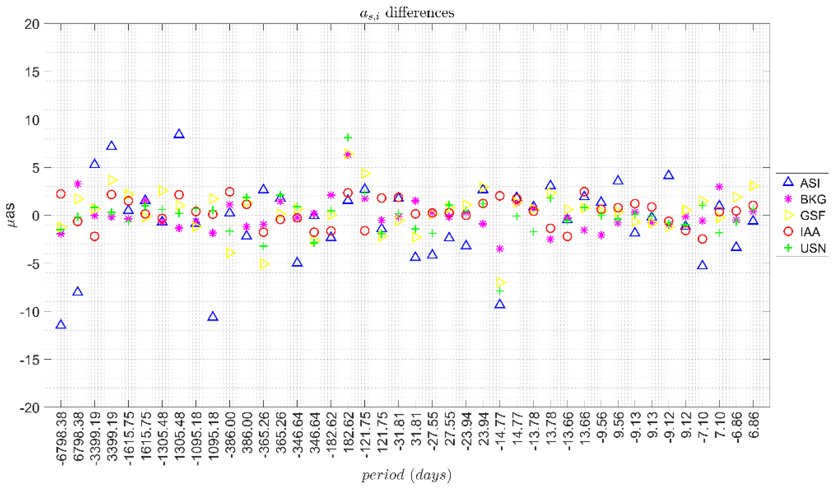
Figure 1 and
Figure 2 show for each solution the differences between the corrections derived from the ICRF3 and ICRF2 series, for
ac,i and
as,i respectively.
In general, the differences were in a band of ±5 μas for all the periods, except for the ASI solution which showed a more scattered behaviour.
Table 3 includes the range of the corrections for each AC together with the mean formal error of the residuals in brackets. It also includes the solution (ICRF2 and ICRF3) and the median and standard deviation (STD) of the differences between the corrections estimated with the series associated to each ICRF.
The median values of the corrections presented a similar behaviour regardless of the ICRF used. The median value of the range (i.e., the difference between the highest correction and the smallest correction with their sign for the 42 terms) for the ac,i amplitudes was 22.3 μas for ICRF2 and 26.1 μas for ICRF3. For the as,i amplitudes, the median value was 26.7 μas for ICRF2 and 28.0 μas for ICRF3. The analysis of the range of the corrections was aimed at noting the magnitude of the estimated corrections and also at pointing out the consistency between the different AC solutions.
The differences between the corrections had a median value of −0.1 μas and standard deviation of 2.0 μas for ac,i amplitudes and a median of 0.4 μas with standard deviation of 1.7 μas for as,i amplitudes. Finally, it should be noted that the use of ICRF3 did not improve the formal error of each computed correction. The mean formal error over all the AC solutions was 2.2 μas for both ICRF2 and ICRF3. In addition, no significant difference was found between the solutions of the different ACs.
From these results it can be concluded that the difference between using ICRF2 or ICRF3 was in the level of a few μas (band of ±5 μas) whereas the estimated values of lunisolar nutation corrections were in the order of a few tens of μas. Therefore, the choice of ICRF for the estimation of corrections to the nutation model had an impact of one order of magnitude less than the magnitude of such corrections.
3.2. Test B: Different CPO Weigthing
In the results presented in the previous section, no stochastic model was used in the least-squares adjustment to estimate the corrections to the nutation model, whereas [
5,
6] used weights taken as the inverse of the squared formal errors from the VLBI series. Additionally, Ref. [
5] estimated a scale factor and an error floor together with the fitting of the corrections in order to account for the differences in the observation geometry between VLBI sessions.
One of the main factors that impacts VLBI estimates of EOPs is the network geometry, and this fact can be taken into consideration in the estimation of corrections to the IAU 2000A model from VLBI-based CPO series [
14]. For this purpose, the CPO precision as a function of the network of the corresponding VLBI session needs to be rescaled and this information can be used to build a stochastic model.
The relationship between network geometry and EOP precision was already addressed by [
14]. Following an analysis of the VLBI series from June 1996 to February 2007, the authors found that the volume of network (
V) could be used as an indicator of the uncertainties in EOP estimation. In order to have consistent uncertainties between sessions, they should be reduced to the unit volume of the network as follows:
where
σm is the modified uncertainty,
σ is the original uncertainty,
V is the volume of the network and
c is a parameter that relates EOP precision and network volume. This value can be fitted using long-term series of VLBI EOP estimates, as will be detailed later.
In order to have consistent uncertainties to build an appropriate stochastic model, we have followed the same methodology as [
14], extending the analyzed period to fit a new model that relates network volume and uncertainty. As a proof of concept, we used GSF series (gsf2020a.eoxy) in the period 1993–2021. The reason for using only one solution was that in this case the factor under analysis was the geometry of the observing network, which was not AC dependent. The geometry of the sessions was the same for all ACs.
The following computations were carried out based on [
14]:
1. For each session of the series, the tetrahedron mesh corresponding to the network polyhedron was defined by means of the Delaunay triangulation. The list of stations in each session was extracted from the EOP series, which included the two-letter IVS station identifiers. The Delaunay triangulation was computed using MATLAB [
15].
2. Computation of the volume of each tetrahedron (
vi):
where
ri is the geocentric station vector. Sessions that had less than four stations were not considered in the analysis.
3. Computation of the total network volume (V) as the sum of the volumes of all the tetrahedrons computed in the previous step.
4. The EOP series were binned in nine groups based on the total network volume in Mm3
5. For each group, the average network volume (
and average CPO uncertainties (
,
) were computed, obtaining the values in
Table 4.
6. Least-squares fitting of a power model relating CPO precision (
σ) and network volume (
V) with the following form:
where
b and
c are the parameters to be estimated. This fitting was applied for
dX and
dY separately, and the results are shown in
Table 5. The value of
c was within the same order of magnitude as the one obtained by [
14] for a shorter period of analysis (−0.238). The difference in the
b value ([
14] reported −0.772 for
dX and −0.772 for
dY) could be due to the number of sessions considered in the analysis (1440 in [
14] and 2268 in this work).
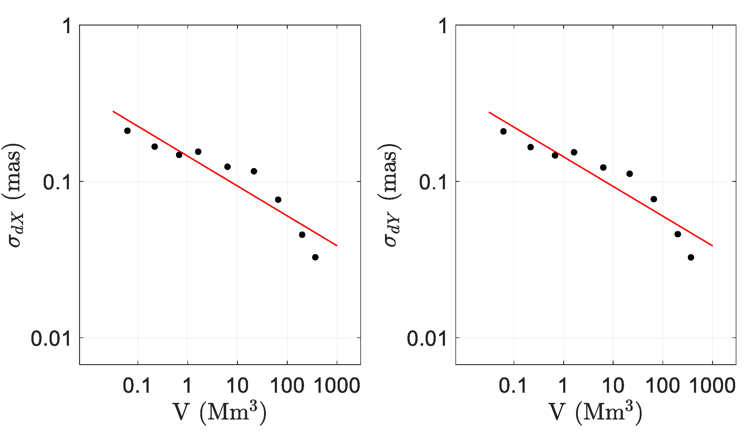
Figure 3 shows the relationship between CPO precision and network volume. Dots correspond to the logarithmic values of
Table 4 and the solid line is the fitted model. Logarithmic scales were used on both axes. This figure was similar to the one obtained by [
14] for a shorter period of analysis and it also showed a clear relationship between CPO precision and network volume.
It was possible to perform a comparison of the effect of the three different stochastic models in the weighted least-squares adjustment to estimate corrections to the nutation model. The three scenarios analysed were the following:
Two statistical criteria were used in order to compare the results of the different strategies evaluated on the CPO weighting:
A posteriori variance factor (): quotient between the sum of each weighted residual square and the number of degrees of freedom of the least-squares fitting.
χ2 value quotient between the a posteriori variance and the a priori variance factor. Values of χ2 close to one indicated a realistic adjustment in terms of a priori weights.
The results obtained in the three scenarios analysed are shown in
Table 6, where it can be seen that the test in which the modified uncertainties were used to build the stochastic model brought the smallest a posteriori variance factor and the χ
2 value closest to 1. Therefore, it can be stated that this was the most suitable stochastic model to be used in the weighted least-squares adjustment to estimate corrections to the nutation model. The improvement in the formal error of the corrections is below μas when using this approach.
Finally,
Table 7 includes the statistics of the differences in the corrections considering the best option (Test B.3) with respect the other two tests performed on the CPO weighting. From these results, it can be concluded that the choice of the stochastic model produced significant differences in the corrections since they were in the μas level, which was the level of the accuracy of the IAU 2000A nutation model
The corrections computed in Test B.3 (modified uncertainties) presented median differences with respect to the other two tests in level of 1 μas or below, standard deviation between 4–5 μas and a range in differences of a few tens of μas. This range was computed as the difference between the highest correction difference and the smallest correction difference with their sign.


