
Evaluation of a New Lightweight UAV-Borne Topo-Bathymetric LiDAR for Shallow Water Bathymetry and Object Detection


Abstract
:1. Introduction
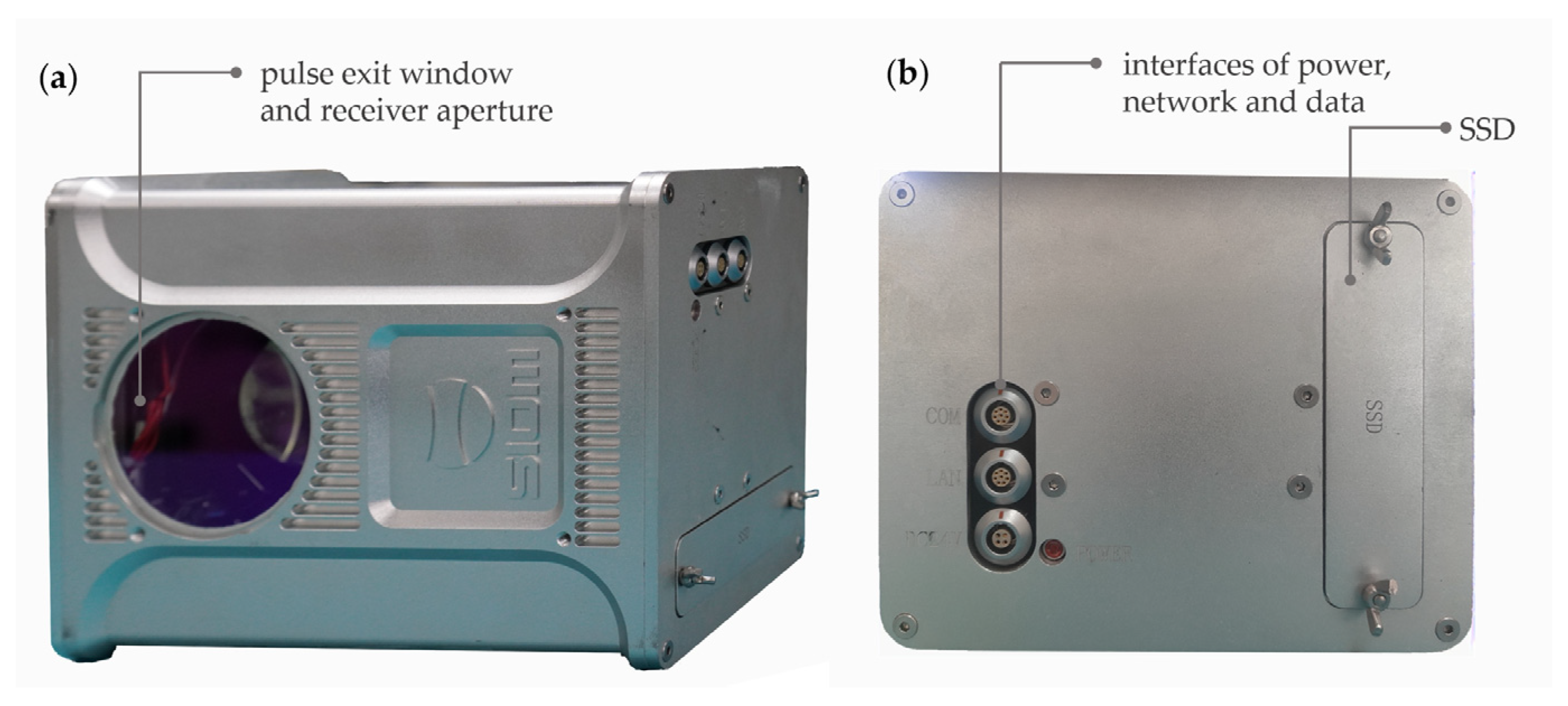
2. Mapper4000U
3. Materials and Methods
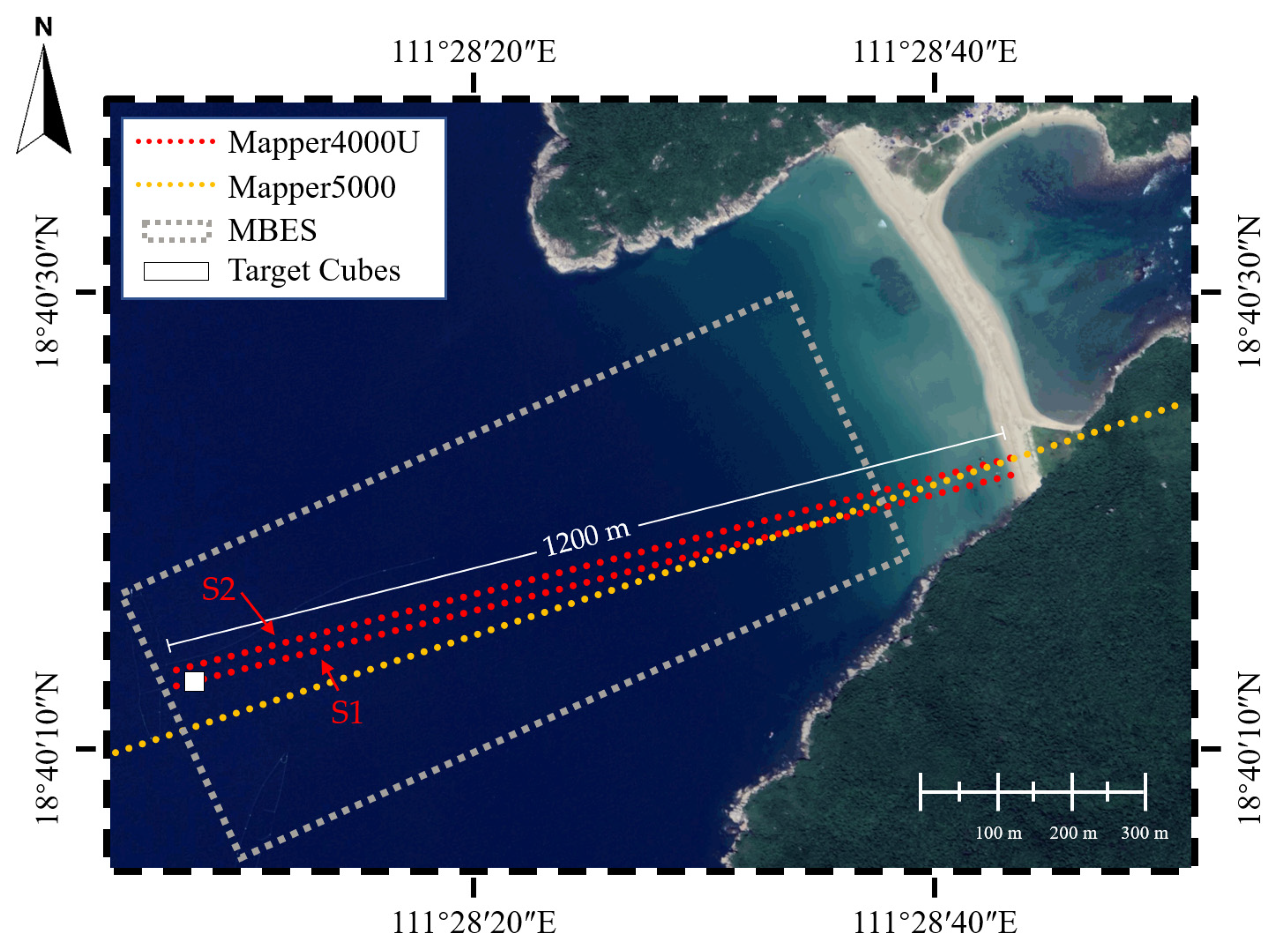
3.1. Study Area
3.2. Field Data
- 1.
- For the accuracy assessment, the study area was also measured by a MBES (Hydro-tech Marine MS400), and a digital bathymetric model (DBM) [29] with high-resolution (0.2 m) was generated using the supporting software. The DBM was used as reference data of water bottom points in this experiment. The geographic coordinates of both the reference DBM and Mapper4000U survey points used the WGS84 ellipsoid and were projected into UTM zone 49 N.
- 2.
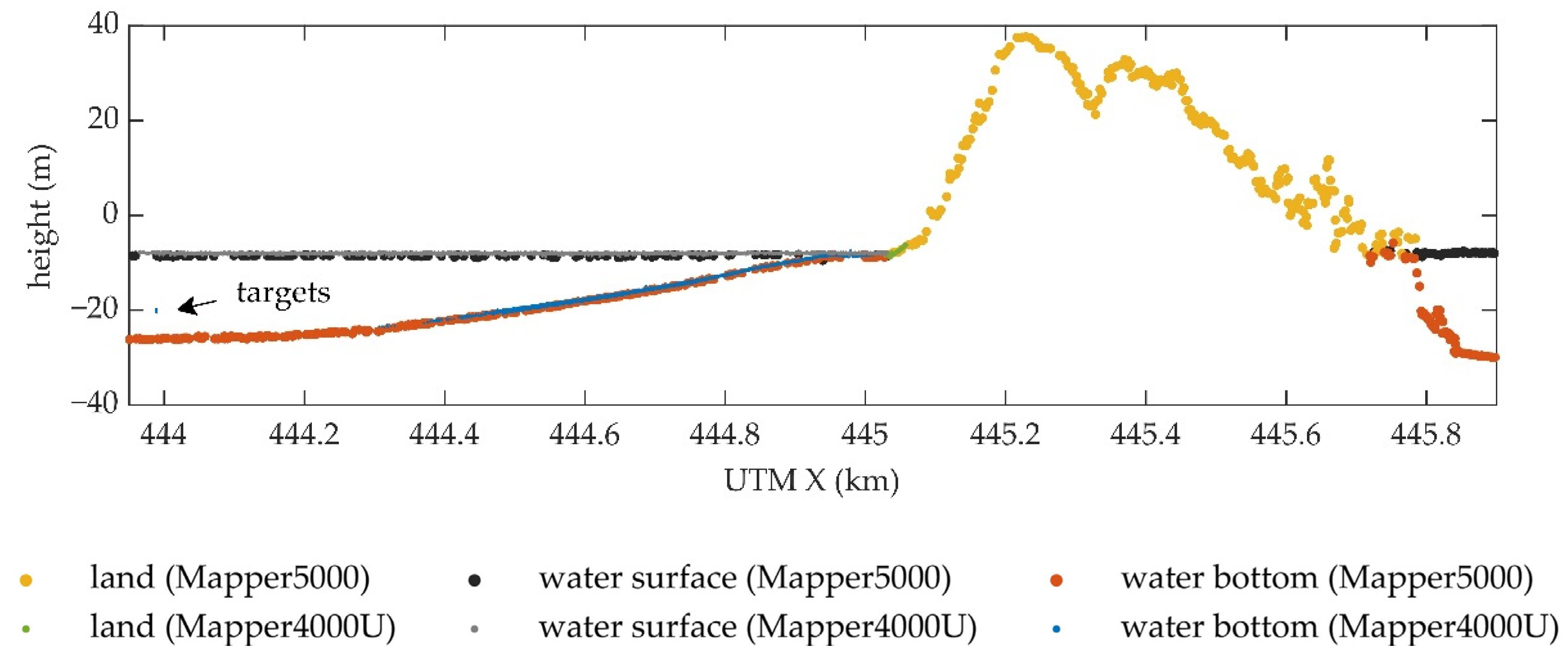
- For the bathymetric performance comparison, a Mapper5000 survey were performed a few days after the UAV survey. The flight altitude, speed, and swath width are much higher than that of the UAV, but the point density is sharply decreased. The data acquisition parameters are compared in Table 3. In data processing, a depth-adaptive waveform decomposition method was used for signal detection, and a post-processing software developed by the manufacturer was used for point cloud generation, including geo-calibration and refraction correction [27]. For comparison, the measured points were also transformed to the geographic coordinates (WGS84).
- 3.
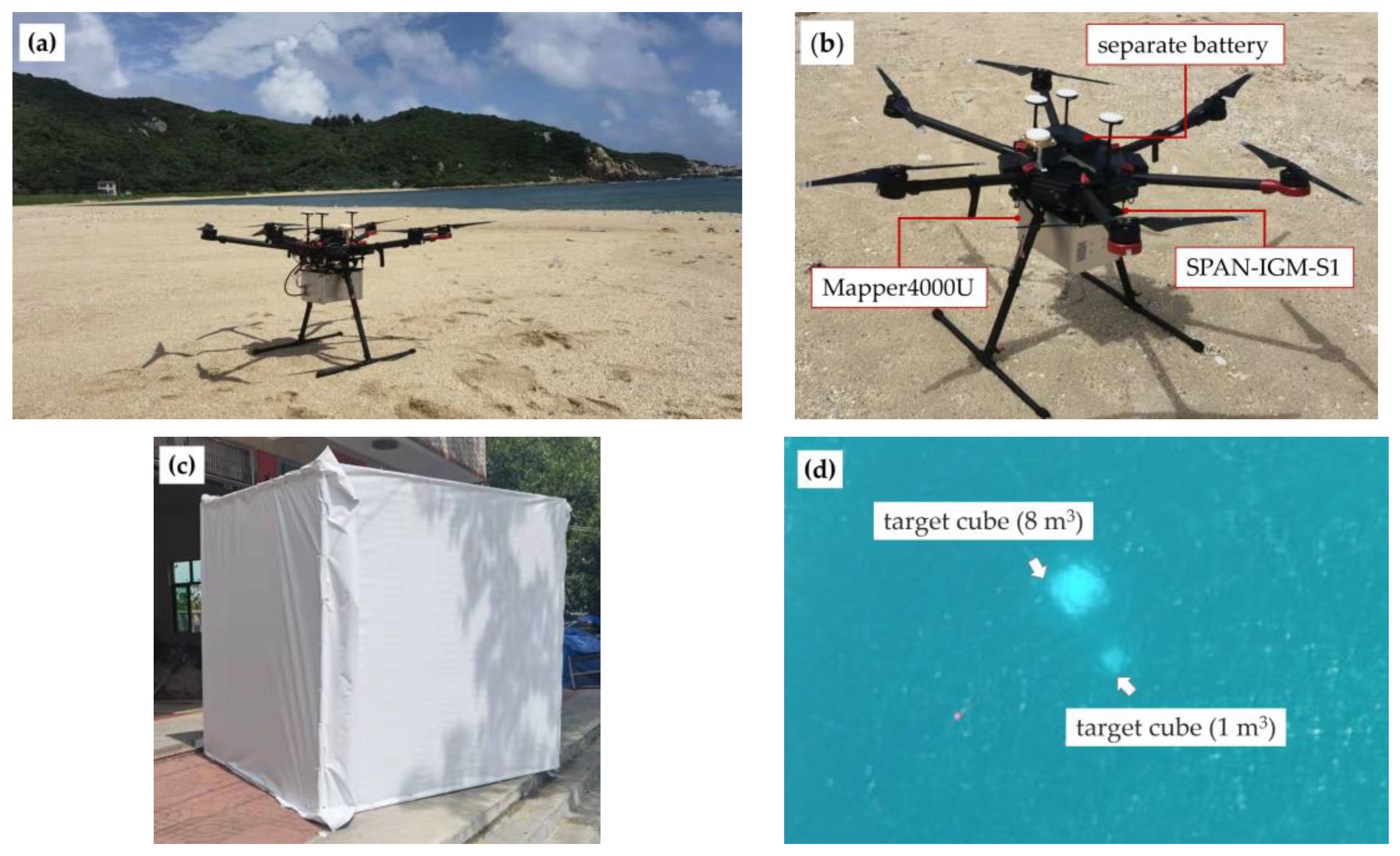
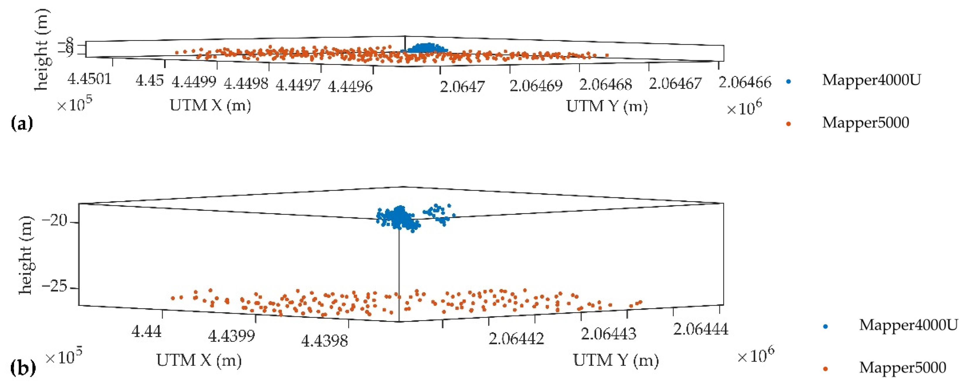
- Small object detection capability. Two fabric targets, a 1-m white cube and a 2-m white cube, were placed in water one day before the UAV survey, and the location of the targets was measured at the same time. The cubes gradually sank to a depth of about 12 m, which was deeper than the Secchi depth.
3.3. Data Processing of the UAV-Borne ALB
- 1.
- POS data processing. The observations from the POS mounted on the platform and a temporary reference station were processed using Waypoint Inertial Explorer8.8 Software to estimate the flight trajectory.
- 2.
- Waveform data processing. The full waveforms were sampled and recorded by the receiver. To extract the signals, a fast and simplified processing method was applied to the received waveforms (see below for a detailed description).
- 3.
- System calibration. The system calibration was conducted in a nearby village. Six strips of Mapper4000U data were collected, and a number of control points were measured by RTK GNSS survey. Thus, the extrinsic error was corrected based on the planar calibration model [30].
- 4.
- Coordinates calculation. Based on the flight trajectory, the extrinsic parameters, and the refraction correction model [27], the detected signals were converted to the 3D point cloud in the WGS_1984_UTM_Zone_49N coordinate.
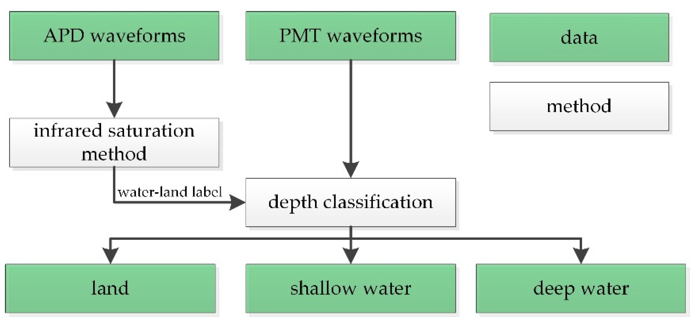
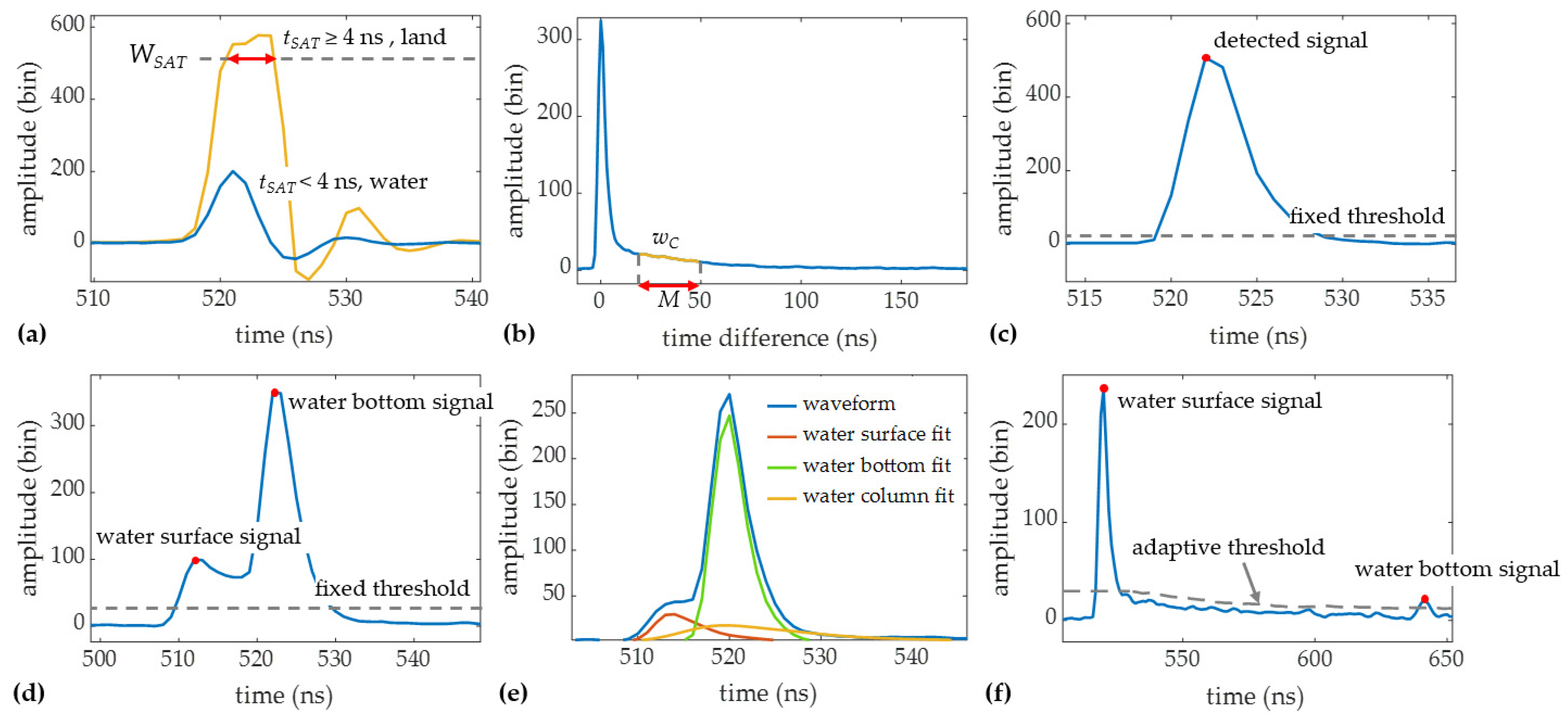
- Shallow water waveforms processing. Shallow water waveforms are first processed using the same methods as the land waveforms for signal detection. If the number of detected signals is greater than or equal to 2, the first signal will be recorded as the water surface signal, and the last signal will be recorded as the water bottom signal, as shown in Figure 5d. If only one signal can be detected, which occurs when the water depth is extremely shallow, the waveform will be decomposed based on an empirical model [27] to extract the water surface and bottom signal, as shown in Figure 5e.
- Deep-water waveforms processing. Denoising is the key to deep water waveforms processing, while the existing waveform filtering methods cannot appropriately deal with the high-intensity noise in the water column scattering. Thus, the fixed threshold in the signal detection method is replaced by a depth-adaptive threshold derived from the truncated water column scattering waveform [27], which greatly reduces the effect of noise in the water column scattering. The intensities of the detected signal are subtracted from the depth-adaptive threshold, and the two signals with the highest strength are selected as the water surface and bottom signal, as shown in Figure 5f.
3.4. Methods for the Evaluation
- 1.
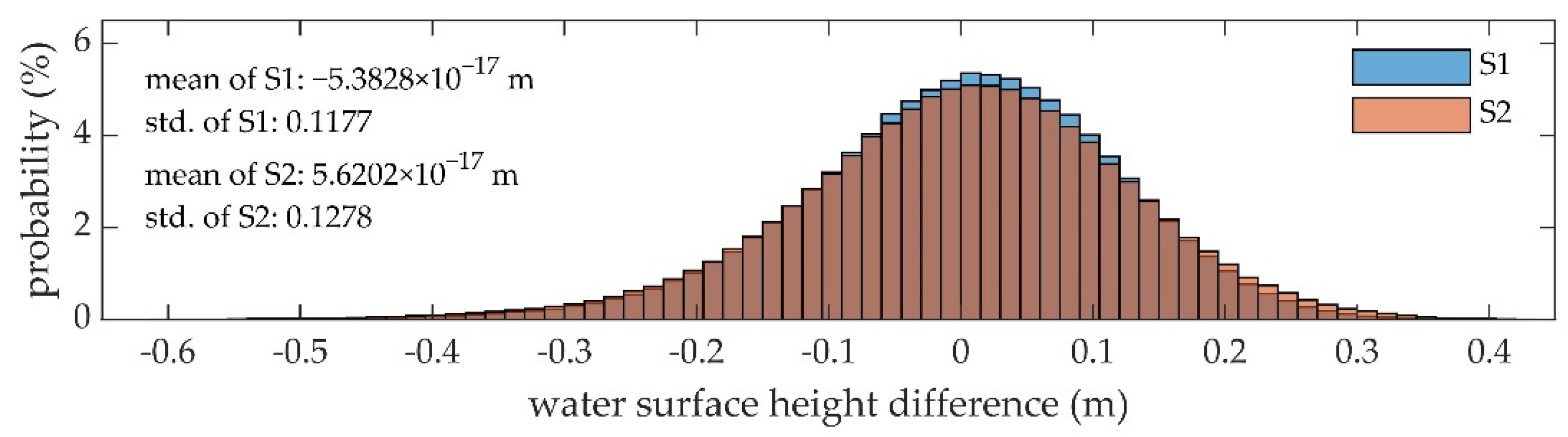
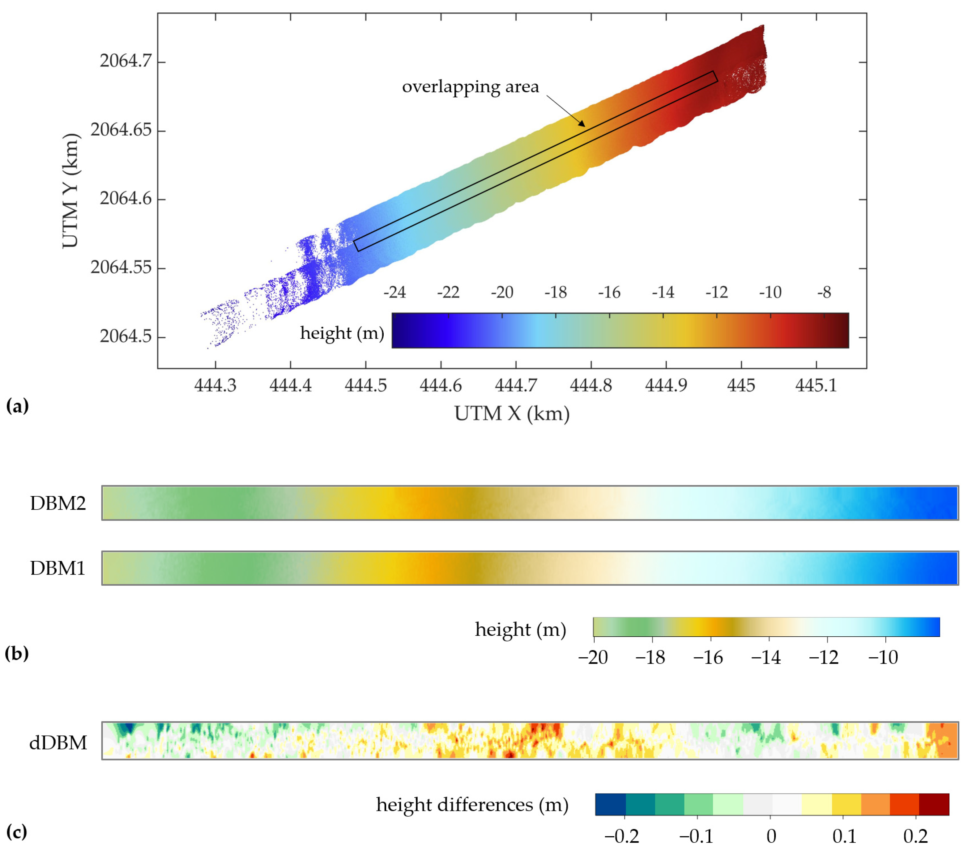
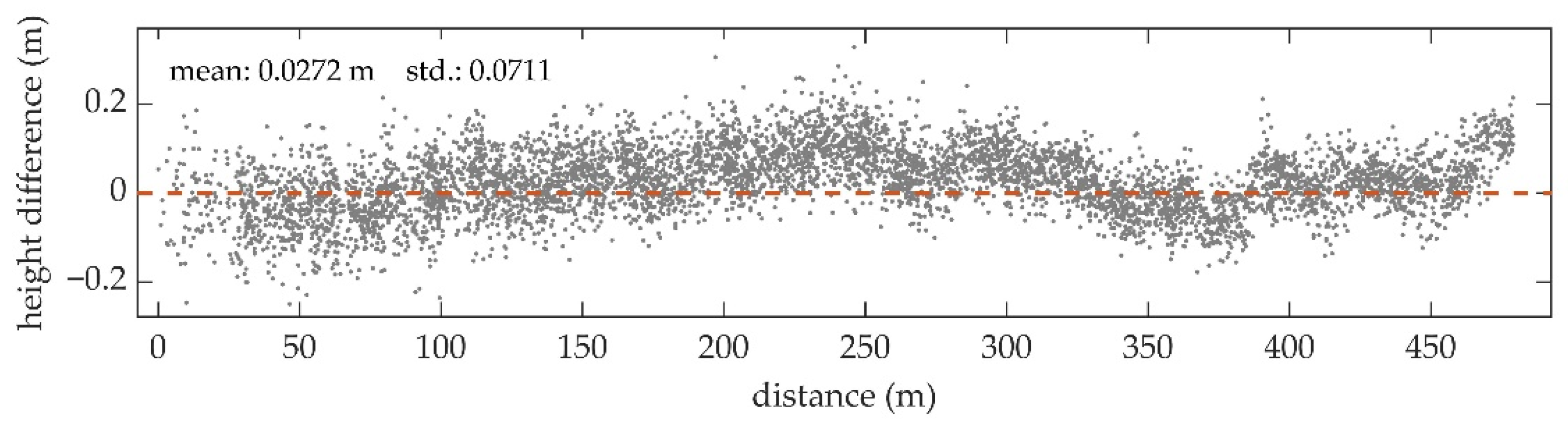
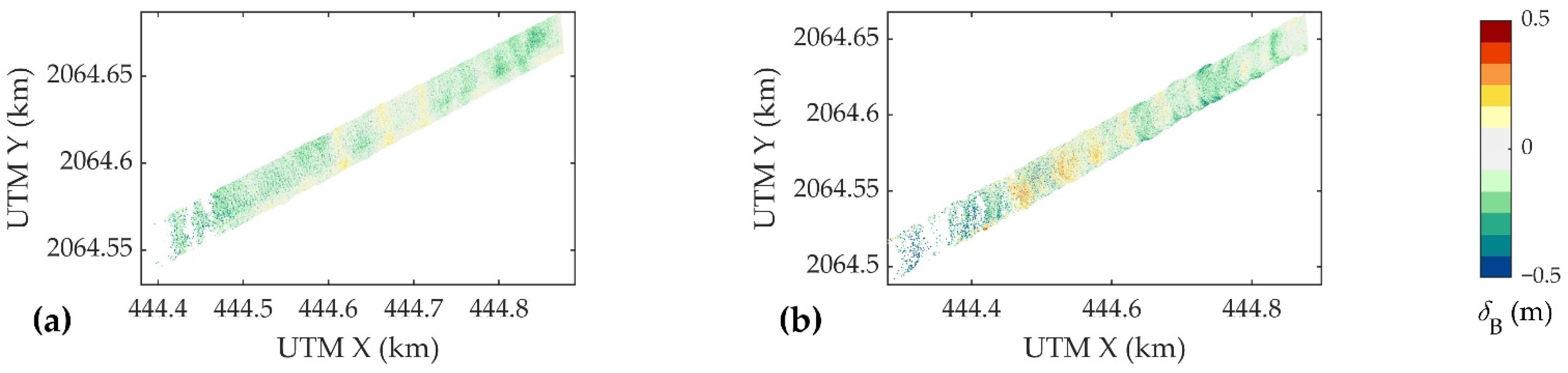
- Precision: Analysis of the relative accuracy of the measurements. The water surface points of each strip were searched in 1 m × 1 m grids based on the planimetric coordinates. In each grid, the points were fitted to a plane, and the distance from the point to the plane was calculated to estimate the ranging precision. In addition, the DBMs of the water bottom were generated via the moving least squares interpolation and compared in the overlapping area of the two strips to evaluate the consistency of the data.
- 2.
- Accuracy: Assessment of the UAV system’s bathymetric accuracy. As the bathymetric LiDAR and MBES only measure instantaneous depths, the depth measurements cannot be directly compared. Therefore, the accuracy was evaluated by comparing the ellipsoid heights of the measured water bottom points with the reference values derived from the DBM generated by MBES measurements in the same planimetric coordinates.
- 3.
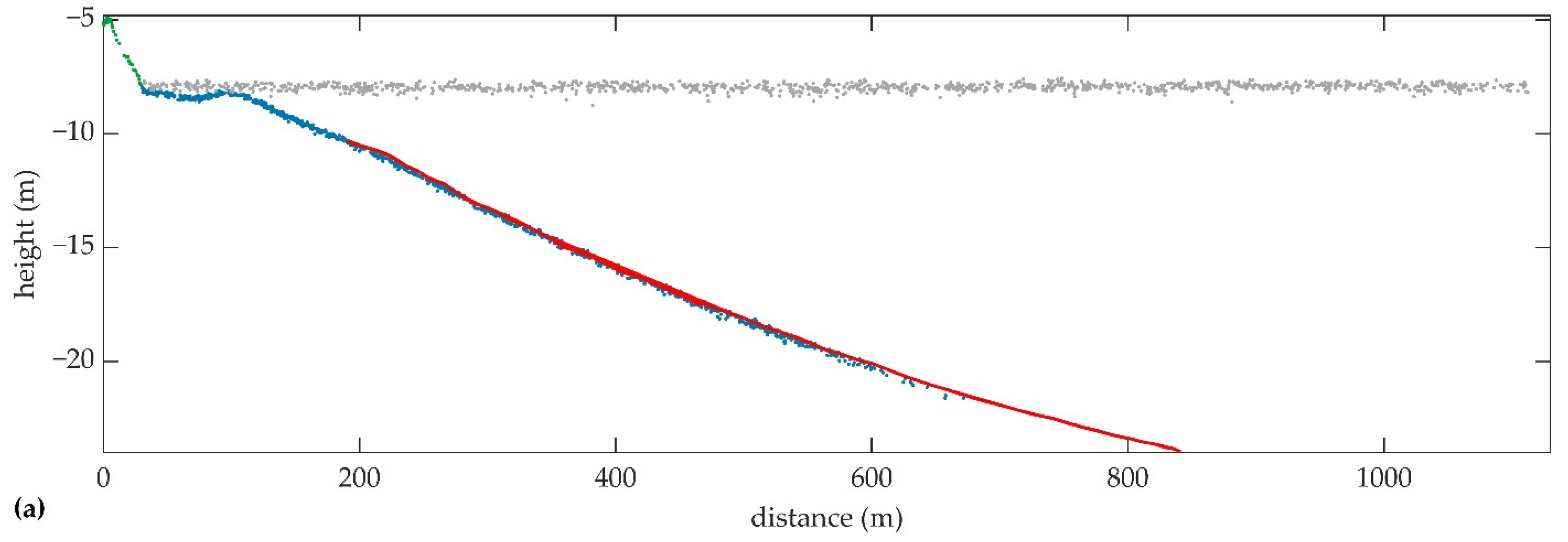
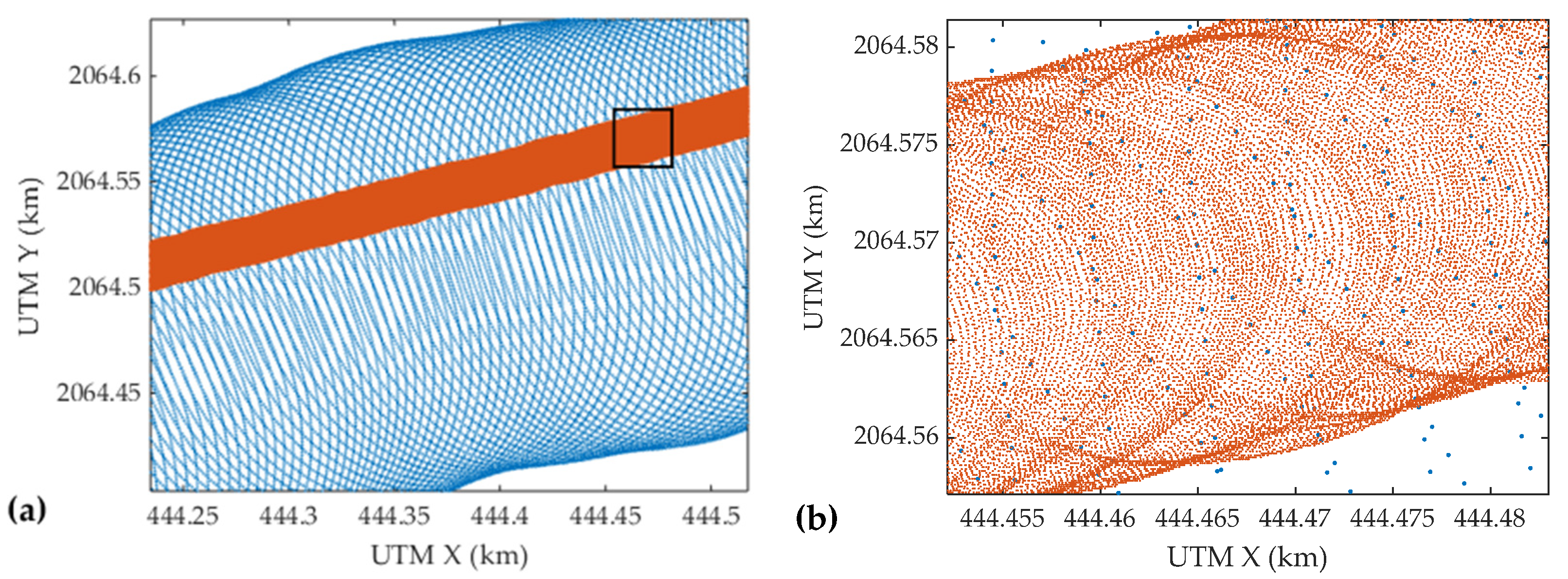
- Bathymetric performance: A comparison of the Mapper4000U and Mapper5000 for bathymetry (including point density, maximum depth penetration, and object detection capability). The point distribution and average density were both considered, and the profiles of the water bottom point clouds obtained from the UAV-borne system and manned platform system were compared. The maximum detected depths of the systems were estimated with the Secchi depth as reference. The capability of small object detection was examined in shallow and deep water.
- 4.
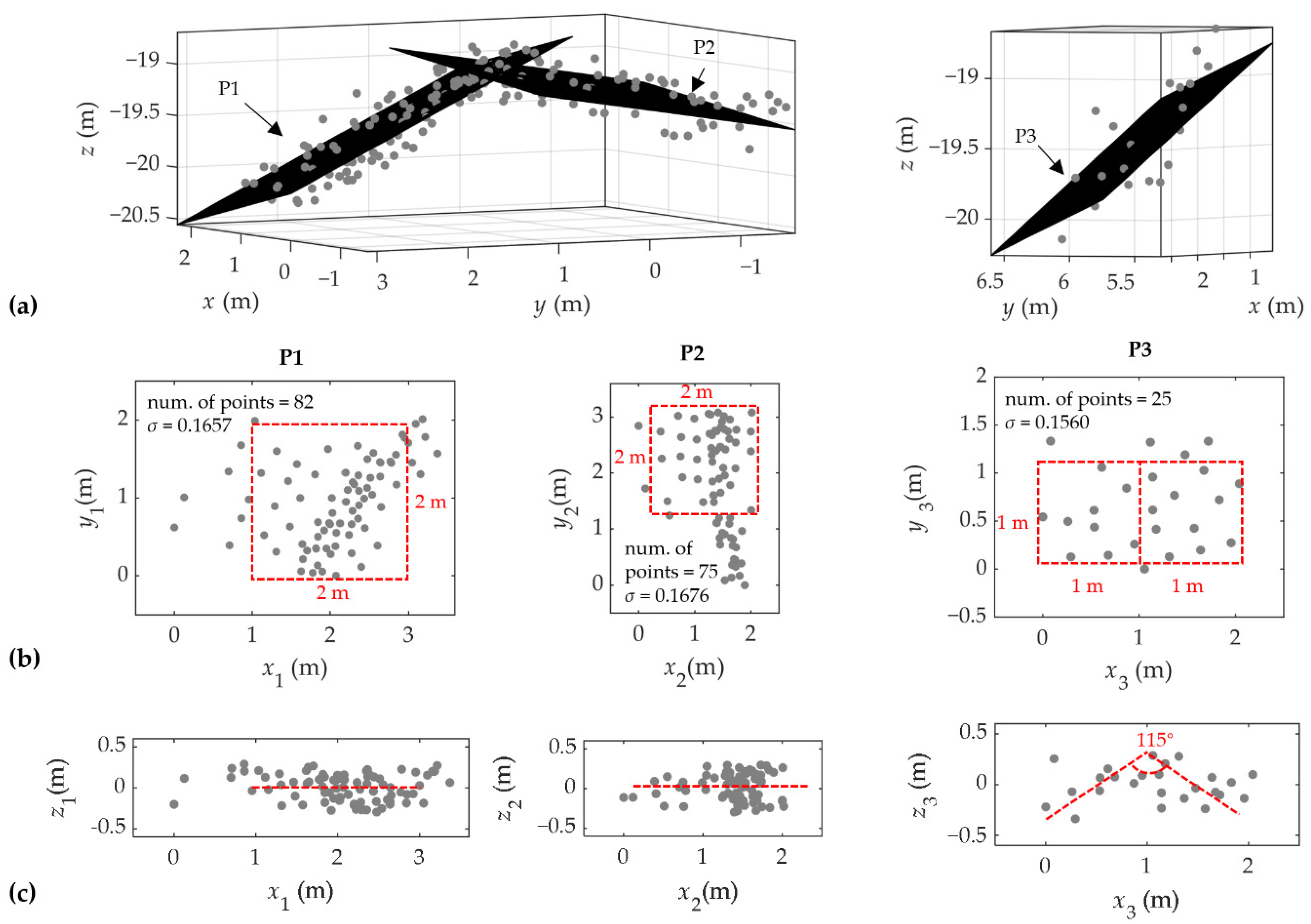
- Object detection capability: The target cube points were extracted from the water bottom point cloud of Mapper4000U and were fitted and projected to planes. To assess the detection accuracy, the distances from the points to the fitted plane and the shape of the projected points were statistically analyzed.
4. Results
4.1. Precision
4.2. Accuracy
4.3. Bathymetric Performance
4.4. Object Detection Capability
5. Discussion
5.1. Environmental Effects on Water Surface Detection
5.2. Consistency between the Adjent Strips
5.3. Impact of In-Water Path Calculation on Water Bottom
5.4. Bathymetric Performance Comparison
5.5. Evaluation of the Object Detection Capability
6. Conclusions
- 1.
- The system can simultaneously acquire land, water surface, and water bottom point clouds with a maximum detectable depth of 1.7–1.9 SD.
- 2.
- The accuracy of the system is evaluated from two aspects, water surface, and bottom. The RMSE of the water surface and bottom heights are 0.1227 m and 0.1268 m, respectively. The detection of the surface signal may be influenced by the water column backscattering, which may also be one of the reasons for the overestimation of water depths. Affected by the calculation error of the in-water path of the laser pulse, errors of water bottom points are dependent on water depths.
- 3.
- Compared to the manned ALB system, this system is lighter and more flexible and can preserve more detailed topographic features with 110 times the point density of the Mapper5000.
- 4.
- For object detection, the system can successfully detect white fabric cubes at a depth of 12 m (beyond 1 SD). The presence of the 1-m target cube and the general shape of the 2-m target cube can be observed in the point cloud. However, shape deformations of the targets also can be observed because of the depth-dependent errors, and the possibility of an object being detected is affected by its reflectance.
Author Contributions
Funding
Acknowledgments
Conflicts of Interest
References
- Guenther, G.C.; Cunningham, A.G.; Laroque, P.E.; Reid, D.J. Meeting the Accuracy Challenge in Airborne Lidar Bathymetry. In Proceedings of the 20th EARSeL Symposium: Workshop on Lidar Remote Sensing of Land and Sea, Dresden, Germany, 16–17 June 2000. [Google Scholar]
- Lague, D.; Feldmann, B. Topo-bathymetric airborne LiDAR for fluvial-geomorphology analysis. In Developments in Earth Surface Processes; Elsevier: Amsterdam, The Netherlands, 2020; Volume 23, pp. 25–54. [Google Scholar] [CrossRef]
- Costa, B.M.; Battista, T.A.; Pittman, S.J. Comparative evaluation of airborne LiDAR and ship-based multibeam SoNAR bathymetry and intensity for mapping coral reef ecosystems. Remote Sens. Environ. 2009, 113, 1082–1100. [Google Scholar] [CrossRef]
- Yunus, A.P.; Dou, J.; Song, X.; Avtar, R. Improved bathymetric mapping of coastal and lake environments using Sentinel-2 and Landsat-8 images. Sensors 2019, 19, 2788. [Google Scholar] [CrossRef] [PubMed] [Green Version]
- Liu, Y.; Deng, R.; Li, J.; Qin, Y.; Xiong, L.; Chen, Q.; Liu, X. Multispectral bathymetry via linear unmixing of the benthic reflectance. IEEE J. Sel. Top. Appl. Earth Observ. Remote Sens. 2018, 11, 4349–4363. [Google Scholar] [CrossRef]
- Kasvi, E.; Salmela, J.; Lotsari, E.; Kumpula, T.; Lane, S.N. Comparison of remote sensing based approaches for mapping bathymetry of shallow, clear water rivers. Geomorphology 2019, 333, 180–197. [Google Scholar] [CrossRef]
- Agrafiotis, P.; Skarlatos, D.; Georgopoulos, A.; Karantzalos, K. DepthLearn: Learning to correct the refraction on point clouds derived from aerial imagery for accurate dense shallow water bathymetry based on SVMs-fusion with LiDAR point clouds. Remote Sens. 2019, 11, 2225. [Google Scholar] [CrossRef] [Green Version]
- Fernandez-Diaz, J.C.; Glennie, C.L.; Carter, W.E.; Shrestha, R.L.; Sartori, M.P.; Singhania, A.; Legleiter, C.J.; Overstreet, B.T. Early results of simultaneous terrain and shallow water bathymetry mapping using a single-wavelength airborne LiDAR sensor. IEEE J. Sel. Top. Appl. Earth Observ. Remote Sens. 2014, 7, 623–635. [Google Scholar] [CrossRef]
- Okhrimenko, M.; Hopkinson, C. A simplified end-user approach to lidar very shallow water bathymetric correction. IEEE Geosci. Remote Sens. Lett. 2019, 17, 3–7. [Google Scholar] [CrossRef]
- Dreier, A.; Janßen, J.; Kuhlmann, H.; Klingbeil, L. Quality analysis of direct georeferencing in aspects of absolute accuracy and precision for a UAV-based laser scanning system. Remote Sens. 2021, 13, 3564. [Google Scholar] [CrossRef]
- Vélez-Nicolás, M.; García-López, S.; Barbero, L.; Ruiz-Ortiz, V.; Sánchez-Bellón, Á. Applications of unmanned aerial systems (UASs) in hydrology: A review. Remote Sens. 2021, 13, 1359. [Google Scholar] [CrossRef]
- Riegl. Riegl BDF-1 Datasheet. 2019. Available online: http://www.riegl.com/uploads/tx_pxpriegldownloads/RIEGL_BDF-1_Datasheet_2019-05-31.pdf (accessed on 15 November 2021).
- ASTRALiTe. ASTRALiTe Edge. 2020. Available online: https://www.astralite.net/edgelidar (accessed on 15 November 2021).
- ASTRALite. ASTRALiTe Demonstrates Scanning Topo–Bathy LiDAR System on DJI Matrice 600 Pro. 2018. Available online: https://www.businesswire.com/news/home/20181119005609/en/ASTRALiTe-Demonstrates-Scanning-Topo%E2%80%93Bathy-LiDAR-System-on-DJI-Matrice-600-Pro (accessed on 15 November 2021).
- Mandlburger, G.; Pfennigbauer, M.; Wieser, M.; Riegl, U.; Pfeifer, N. Evaluation of a novel UAV-borne topo-bathymetric laser profiler. Int. Arch. Photogramm. Remote Sens. Spat. Inf. Sci. 2016, XLI-B1, 933–939. [Google Scholar] [CrossRef] [Green Version]
- Fuchs, E.; Mathur, A. Utilizing circular scanning in the CZMIL system. In Algorithms Technol. Multispectral, Hyperspectral, Ultraspectral Imagery XVI, Proceedings of the SPIE Defense, Security, and Sensing, Orlando, FL, USA, 5–9 April 2010; SPIE: Bellingham, WA, USA, 2010; Volume 7695, p. 76950W. [Google Scholar] [CrossRef]
- Fugro. RAMMS Flyer. 2020. Available online: https://www.fugro.com/Widgets/MediaResourcesList/MediaResourceDownloadHandler.ashx?guid=eebbbdf2-f3db-6785-9f9d-ff250019aa6e&culture=en (accessed on 15 November 2021).
- Riegl. Riegl VQ-840-G Datasheet. 2021. Available online: http://www.riegl.com/uploads/tx_pxpriegldownloads/RIEGL_VQ-840-G_Datasheet_2021-09-01.pdf (accessed on 15 November 2021).
- Fugro. Fugro’s New RAMMS Technology Advances Bathymetric Lidar Mapping Capabilities. 2018. Available online: https://lidarmag.com/2018/08/09/fugros-new-ramms-technology-advances-bathymetric-lidar-mapping-capabilities/ (accessed on 15 November 2021).
- Mandlburger, G.; Pfennigbauer, M.; Schwarz, R.; Flöry, S.; Nussbaumer, L. Concept and performance evaluation of a novel UAV-borne topo-bathymetric LiDAR sensor. Remote Sens. 2020, 12, 986. [Google Scholar] [CrossRef] [Green Version]
- Islam, M.T.; Yoshida, K.; Nishiyama, S.; Sakai, K.; Tsuda, T. Characterizing vegetated rivers using novel unmanned aerial vehicle-borne topo-bathymetric green lidar: Seasonal applications and challenges. River Res. Appl. 2021, 38, 44–58. [Google Scholar] [CrossRef]
- Kinzel, P.J.; Legleiter, C.J.; Grams, P.E. Field evaluation of a compact, polarizing topo-bathymetric lidar across a range of river conditions. River Res. Appl. 2021, 37, 531–543. [Google Scholar] [CrossRef]
- Pe’eri, S.; Morgan, L.V.; Philpot, W.D.; Armstrong, A.A. Land-water interface resolved from airborne LiDAR bathymetry (ALB) waveforms. J. Coast Res. 2011, 62, 75–85. [Google Scholar] [CrossRef]
- Zhao, X.; Wang, X.; Zhao, J.; Zhou, F. An improved water-land discriminator using laser waveform amplitudes and point cloud elevations of airborne LIDAR. J. Coast Res. 2021, 37, 1158–1172. [Google Scholar] [CrossRef]
- Mandlburger, G.; Pfeifer, N.; Soergel, U. Water Surface Reconstruction in Airborne Laser Bathymetry from Redundant Bed Observations. In Proceedings of the ISPRS Annals of Photogrammetry, Remote Sensing & Spatial Information Sciences, Wuhan, China, 8–22 September 2017. [Google Scholar] [CrossRef] [Green Version]
- Zhao, J.; Zhao, X.; Zhang, H.; Zhou, F. Shallow water measurements using a single green laser corrected by building a near water surface penetration model. Remote Sens. 2017, 9, 426. [Google Scholar] [CrossRef] [Green Version]
- Xing, S.; Wang, D.; Xu, Q.; Lin, Y.; Li, P.; Jiao, L.; Zhang, X.; Liu, C. A depth-adaptive waveform decomposition method for airborne LiDAR bathymetry. Sensors 2019, 19, 5065. [Google Scholar] [CrossRef] [Green Version]
- Fuchs, E.; Tuell, G. Conceptual design of the CZMIL data acquisition system (DAS): Integrating a new bathymetric lidar with a commercial spectrometer and metric camera for coastal mapping applications. In Algorithms Technol. Multispectral, Hyperspectral, Ultraspectral Imagery XVI, Proceedings of the SPIE Defense, Security, and Sensing, Orlando, FL, USA, 5–9 April 2010; SPIE: Bellingham, WA, USA, 2010; Volume 7695, p. 76950U. [Google Scholar] [CrossRef]
- Guth, P.L.; Van Niekerk, A.; Grohmann, C.H.; Muller, J.-P.; Hawker, L.; Florinsky, I.V.; Gesch, D.; Reuter, H.I.; Herrera-Cruz, V.; Riazanoff, S.; et al. Digital elevation models: Terminology and definitions. Remote Sens. 2021, 13, 3581. [Google Scholar] [CrossRef]
- Yu, J.; Lu, X.; Tian, M.; Chan, T.; Chen, C. Automatic extrinsic self-calibration of mobile LiDAR systems based on planar and spherical features. Meas. Sci. Technol. 2021, 32, 065107. [Google Scholar] [CrossRef]
- Guenther, G.C.; LaRocque, P.E.; Lillycrop, W.J. Multiple Surface Channels in Scanning Hydrographic Operational Airborne Lidar Survey (SHOALS) Airborne LiDAR. In Proceedings of the Ocean Optics XII. International Society for Optics and Photonics, Bergen, Norway, 13–15 June 1994; Volume 2258, pp. 422–430. [Google Scholar] [CrossRef]
- Saylam, K.; Brown, R.A.; Hupp, J.R. Assessment of depth and turbidity with airborne Lidar bathymetry and multiband satellite imagery in shallow water bodies of the Alaskan North Slope. Int. J. Appl. Earth Obs. Geoinf. 2017, 58, 191–200. [Google Scholar] [CrossRef]
- Wagner, W.; Roncat, A.; Melzer, T.; Ullrich, A. Waveform analysis techniques in airborne laser scanning. Int. Arch. Photogramm. Remote Sens. 2007, 36, 413–418. [Google Scholar]
- Höfle, B.; Vetter, M.; Pfeifer, N.; Mandlburger, G.; Stötter, J. Water surface mapping from airborne laser scanning using signal intensity and elevation data. Earth Surf. Processes Landf. 2009, 34, 1635–1649. [Google Scholar] [CrossRef]
- Yang, F.; Su, D.; Yue, M.; Feng, C.; Yang, A.; Wang, M. Refraction correction of airborne LiDAR bathymetry based on sea surface profile and ray tracing. IEEE Trans. Geosci. Remote Sens. 2017, 55, 6141–6149. [Google Scholar] [CrossRef]
- Su, D.; Yang, F.; Ma, Y.; Wang, X.; Yang, A.; Qi, C. Propagated uncertainty models arising from device, environment, and target for a small laser spot airborne lidar bathymetry and its verification in the South China Sea. IEEE Trans. Geosci. Remote Sens. 2019, 58, 3213–3231. [Google Scholar] [CrossRef]
- Birkebak, M.; Eren, F.; Pe’eri, S.; Weston, N. The effect of surface waves on airborne lidar bathymetry (ALB) measurement uncertainties. Remote Sens. 2018, 10, 453. [Google Scholar] [CrossRef] [Green Version]
- Schwarz, R.; Pfeifer, N.; Pfennigbauer, M.; Mandlburger, G. Depth measurement bias in pulsed airborne laser hydrography induced by chromatic dispersion. IEEE Geosci. Remote Sens. Lett. 2020, 18, 1332–1336. [Google Scholar] [CrossRef]
- Alvarez, L.V.; Moreno, H.A.; Segales, A.R.; Pham, T.G.; Pillar-Little, E.A.; Chilson, P.B. Merging unmanned aerial systems (UAS) imagery and echo soundings with an adaptive sampling technique for bathymetric surveys. Remote Sens. 2018, 10, 1362. [Google Scholar] [CrossRef] [Green Version]
- Chowdhury, E.H.; Hassan, Q.K.; Achari, G.; Gupta, A. Use of bathymetric and LiDAR data in generating digital elevation model over the lower Athabasca River watershed in Alberta, Canada. Water 2017, 9, 19. [Google Scholar] [CrossRef] [Green Version]
- Pan, Z.; Glennie, C.L.; Fernandez-Diaz, J.C.; Legleiter, C.J.; Overstreet, B. Fusion of LiDAR orthowaveforms and hyperspectral imagery for shallow river bathymetry and turbidity estimation. IEEE Trans. Geosci. Remote Sens. 2016, 54, 4165–4177. [Google Scholar] [CrossRef]
- Genchi, S.A.; Vitale, A.J.; Perillo, G.M.E.; Seitz, C.; Delrieux, C.A. Mapping topobathymetry in a shallow tidal environment using low-cost technology. Remote Sens. 2020, 12, 1394. [Google Scholar] [CrossRef]
- Lubczonek, J.; Kazimierski, W.; Zaniewicz, G.; Lacka, M. Methodology for combining data acquired by unmanned surface and aerial vehicles to create digital bathymetric models in shallow and ultra-shallow waters. Remote Sens. 2022, 14, 105. [Google Scholar] [CrossRef]
- Wang, C.K.; Philpot, W.D. Using airborne bathymetric lidar to detect bottom type variation in shallow waters. Remote Sens. Environ. 2007, 106, 123–135. [Google Scholar] [CrossRef]
- Feygels, V.; Ramnath, V.; Smith, B.; Kopilevich, Y. Meeting the international hydrographic organization requirements for bottom feature detection using the Coastal Zone Mapping and Imaging Lidar (CZMIL). In Proceedings of the OCEANS 2016 MTS/IEEE Monterey, Monterey, CA, USA, 19–23 September 2016. [Google Scholar] [CrossRef]


| Pulse Repetition Frequency | Pulse Energy | Scan Rate | Size | Weight |
|---|---|---|---|---|
| 4 kHz | 12 μJ@1064 nm 24 μJ@532 nm | 15 lines/s | 235 mm × 184 mm × 148 mm | 4.4 kg |
| Mapper4000U | Mapper5000 | MBES | Target Placement |
|---|---|---|---|
| 26 September | 2 October | 29 September | 25 September |
| System | Altitude | Speed | Swath Width | Point Density | Flight Duration 1 |
|---|---|---|---|---|---|
| Mapper4000U | 50 m | 5 m/s | 21 m | 42 points/m2 | 225 s |
| Mapper5000 | 375 m | 65 m/s | 201 m | 0.38 points/m2 | 22 s |
| Strip | Mean of Height [m] | RMSE [m] | |δS| < 0.3 m [%] |
|---|---|---|---|
| S1 | −7.9452 | 0.1177 | 98.49 |
| S2 | −7.9507 | 0.1278 | 97.49 |
| Sum | −7.9478 | 0.1227 | 98.01 |
| Strip | Max. of Height [m] | Min. of Height [m] | RMSE [m] | Mean of δB [m] | |δB| < 0.3 m [%] |
|---|---|---|---|---|---|
| S1 | −7.9500 | −22.1639 | 0.1075 | −0.0520 | 98.48 |
| S2 | −8.0665 | −24.1038 | 0.1420 | −0.0705 | 93.89 |
| Sum | −7.9500 | −24.1038 | 0.1268 | −0.0615 | 96.11 |
Publisher’s Note: MDPI stays neutral with regard to jurisdictional claims in published maps and institutional affiliations. |
© 2022 by the authors. Licensee MDPI, Basel, Switzerland. This article is an open access article distributed under the terms and conditions of the Creative Commons Attribution (CC BY) license (https://creativecommons.org/licenses/by/4.0/).
Share and Cite
Wang, D.; Xing, S.; He, Y.; Yu, J.; Xu, Q.; Li, P. Evaluation of a New Lightweight UAV-Borne Topo-Bathymetric LiDAR for Shallow Water Bathymetry and Object Detection. Sensors 2022, 22, 1379. https://0-doi-org.brum.beds.ac.uk/10.3390/s22041379
Wang D, Xing S, He Y, Yu J, Xu Q, Li P. Evaluation of a New Lightweight UAV-Borne Topo-Bathymetric LiDAR for Shallow Water Bathymetry and Object Detection. Sensors. 2022; 22(4):1379. https://0-doi-org.brum.beds.ac.uk/10.3390/s22041379
Chicago/Turabian StyleWang, Dandi, Shuai Xing, Yan He, Jiayong Yu, Qing Xu, and Pengcheng Li. 2022. "Evaluation of a New Lightweight UAV-Borne Topo-Bathymetric LiDAR for Shallow Water Bathymetry and Object Detection" Sensors 22, no. 4: 1379. https://0-doi-org.brum.beds.ac.uk/10.3390/s22041379