


Cherenkov Radiation in Optical Fibres as a Versatile Machine Protection System in Particle Accelerators
 , , , , ,
Abstract
:1. Introduction
2. Materials and Methods
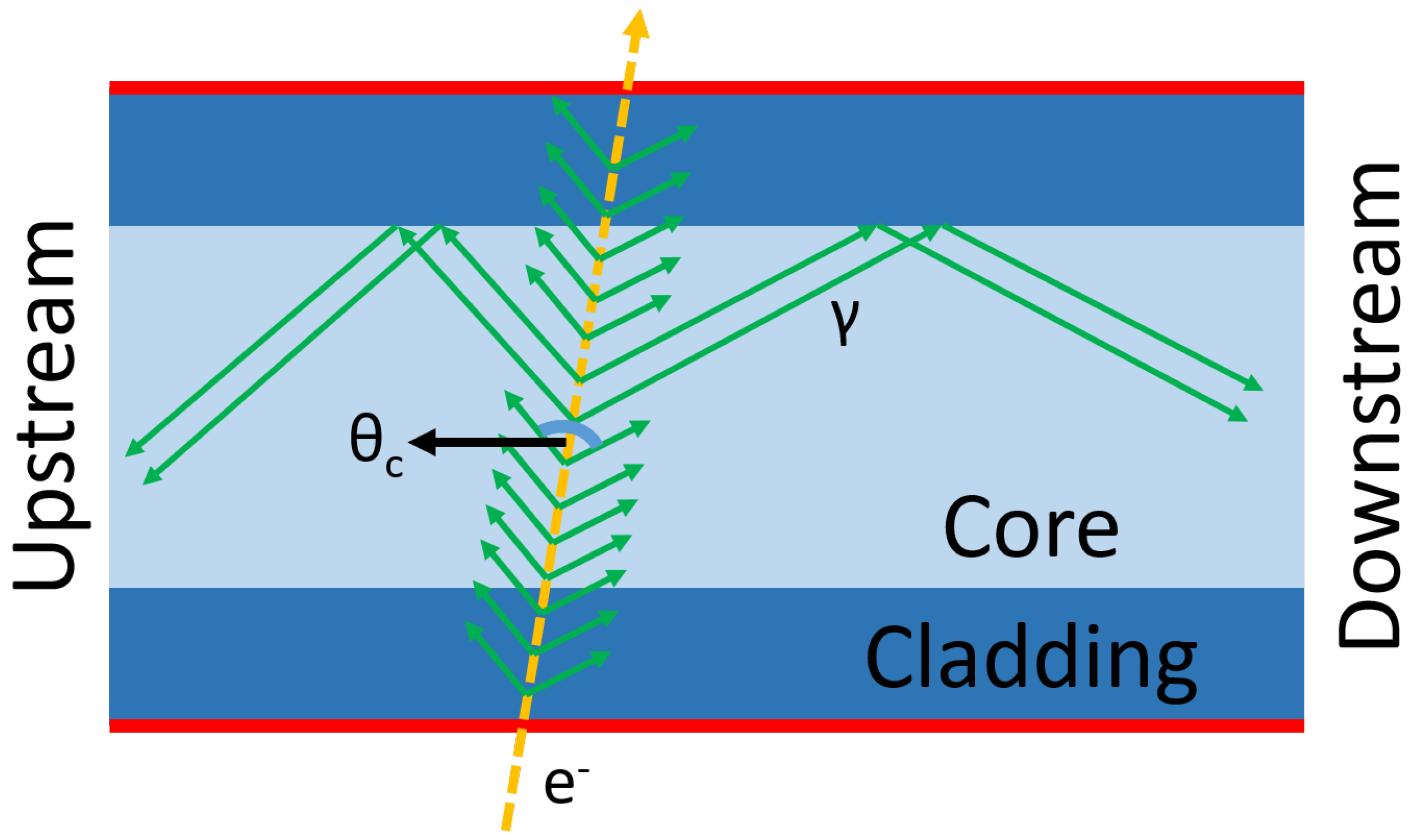
2.1. Detection Mechanism
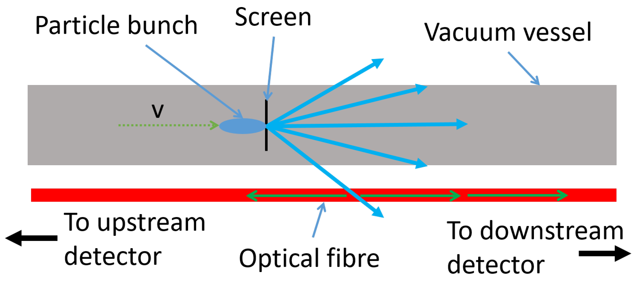
2.2. Application to Beam Loss
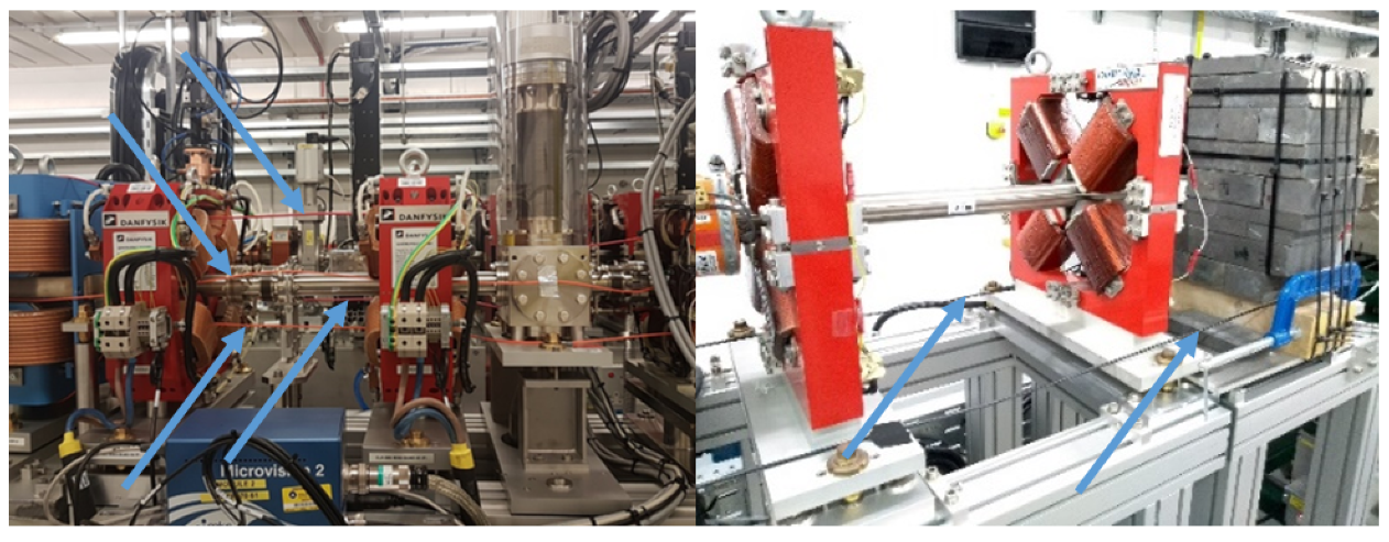
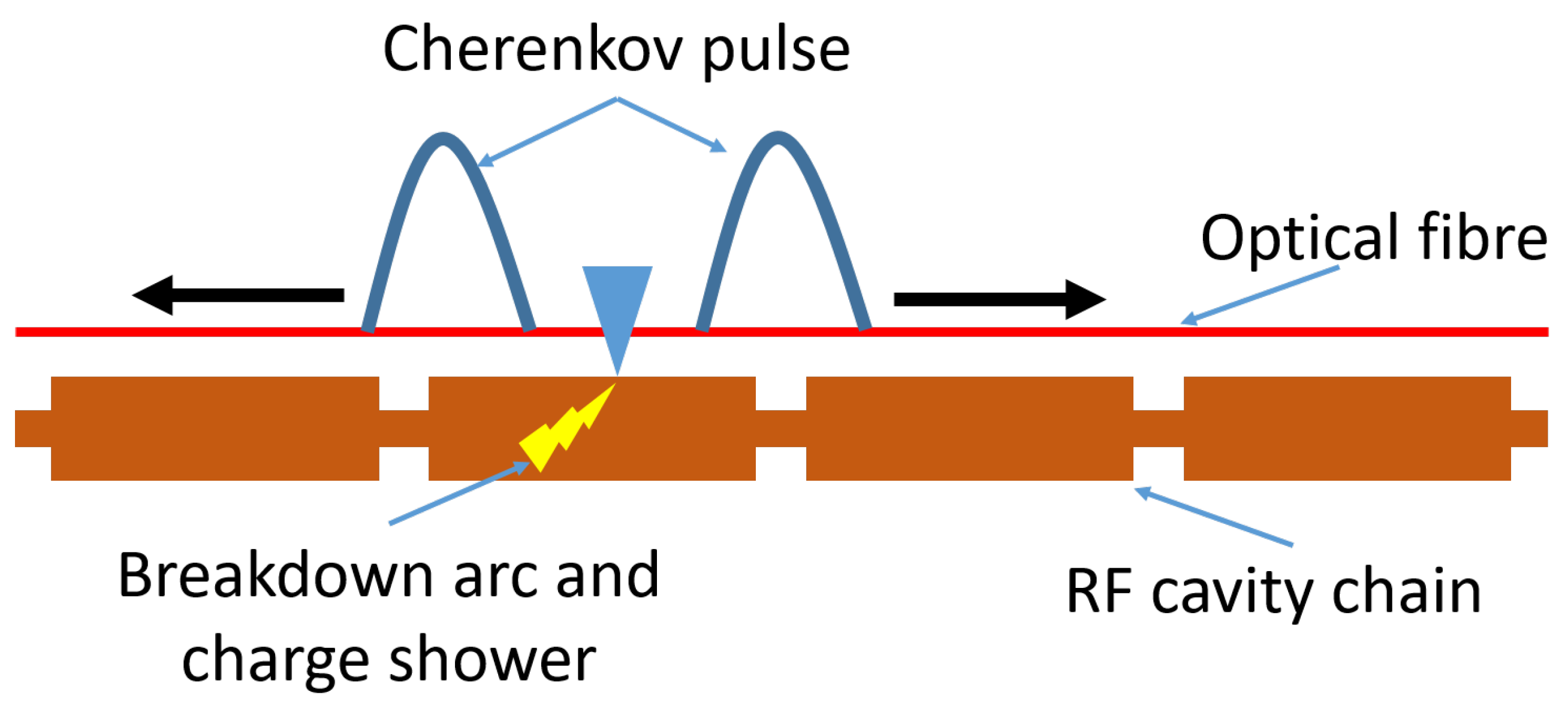
2.3. Application to RF Breakdown
3. Results
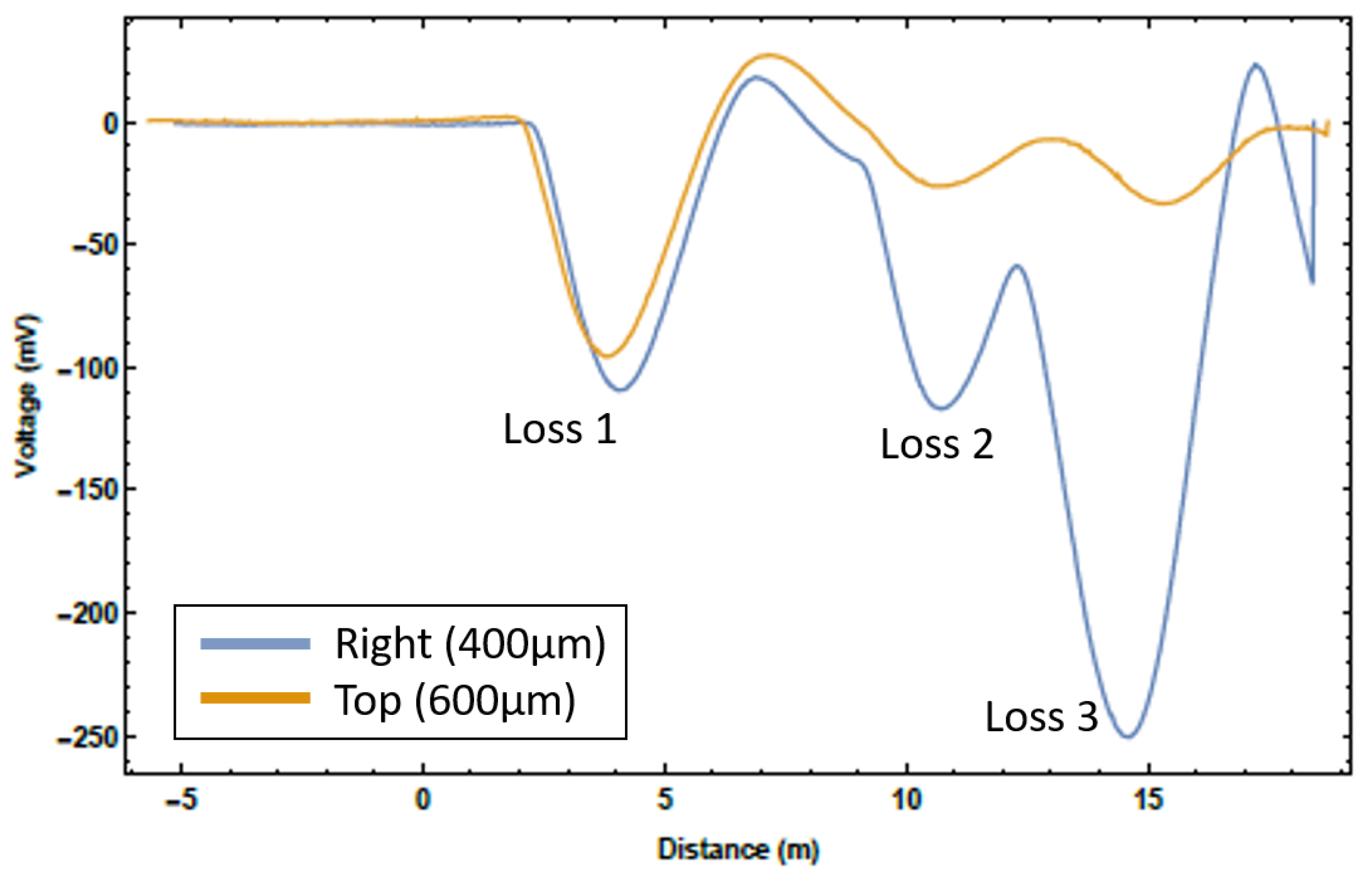
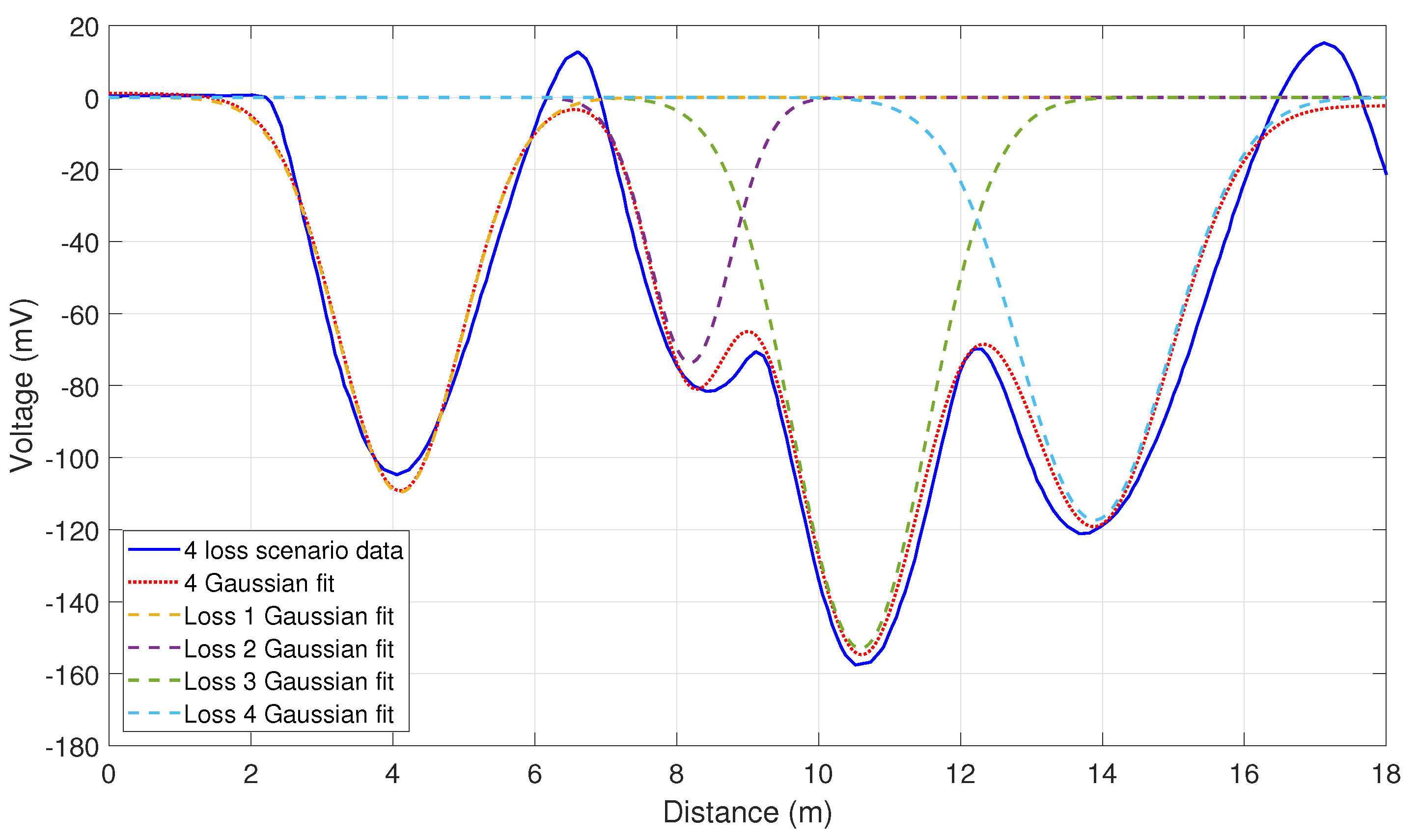
3.1. Beam Loss Monitoring
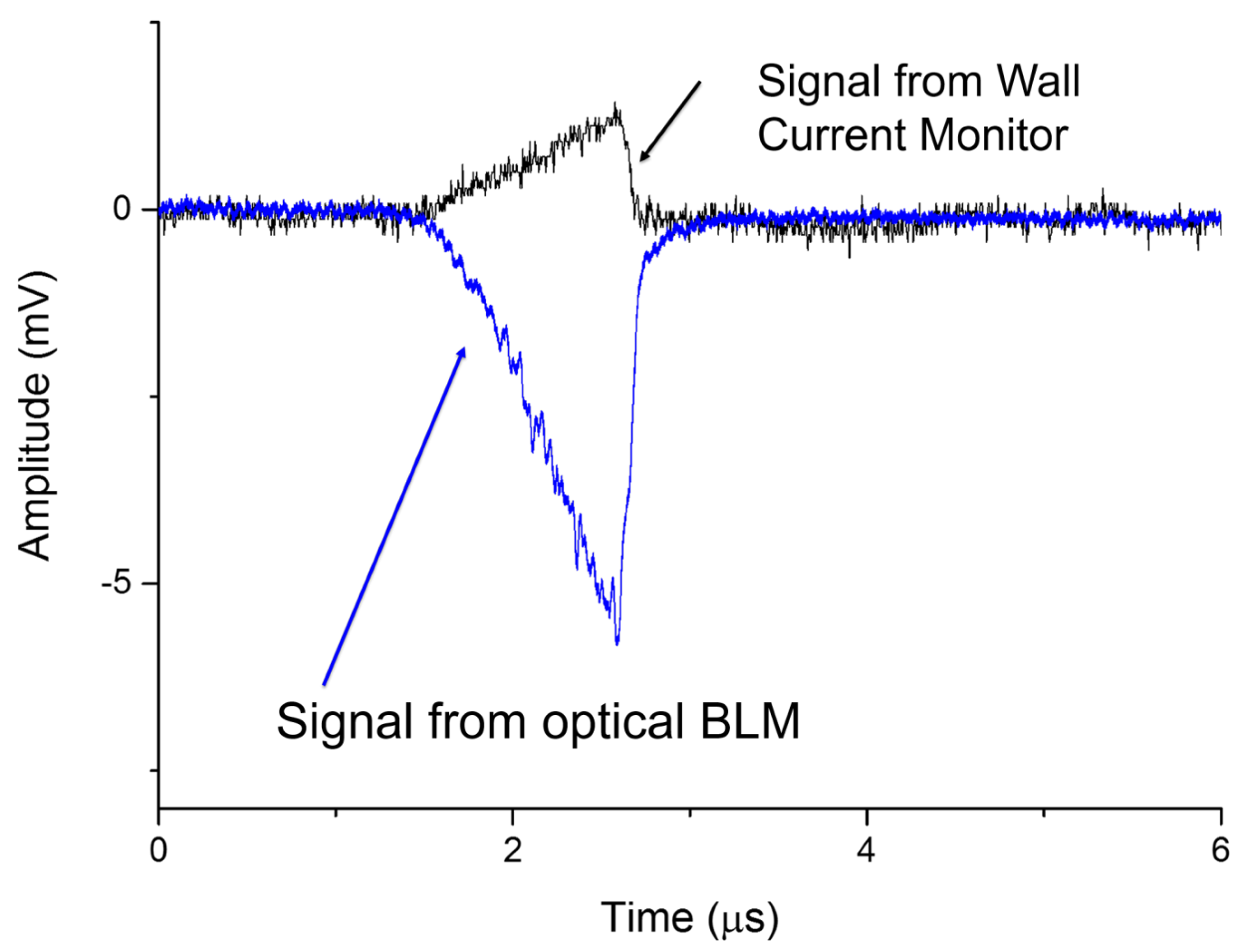
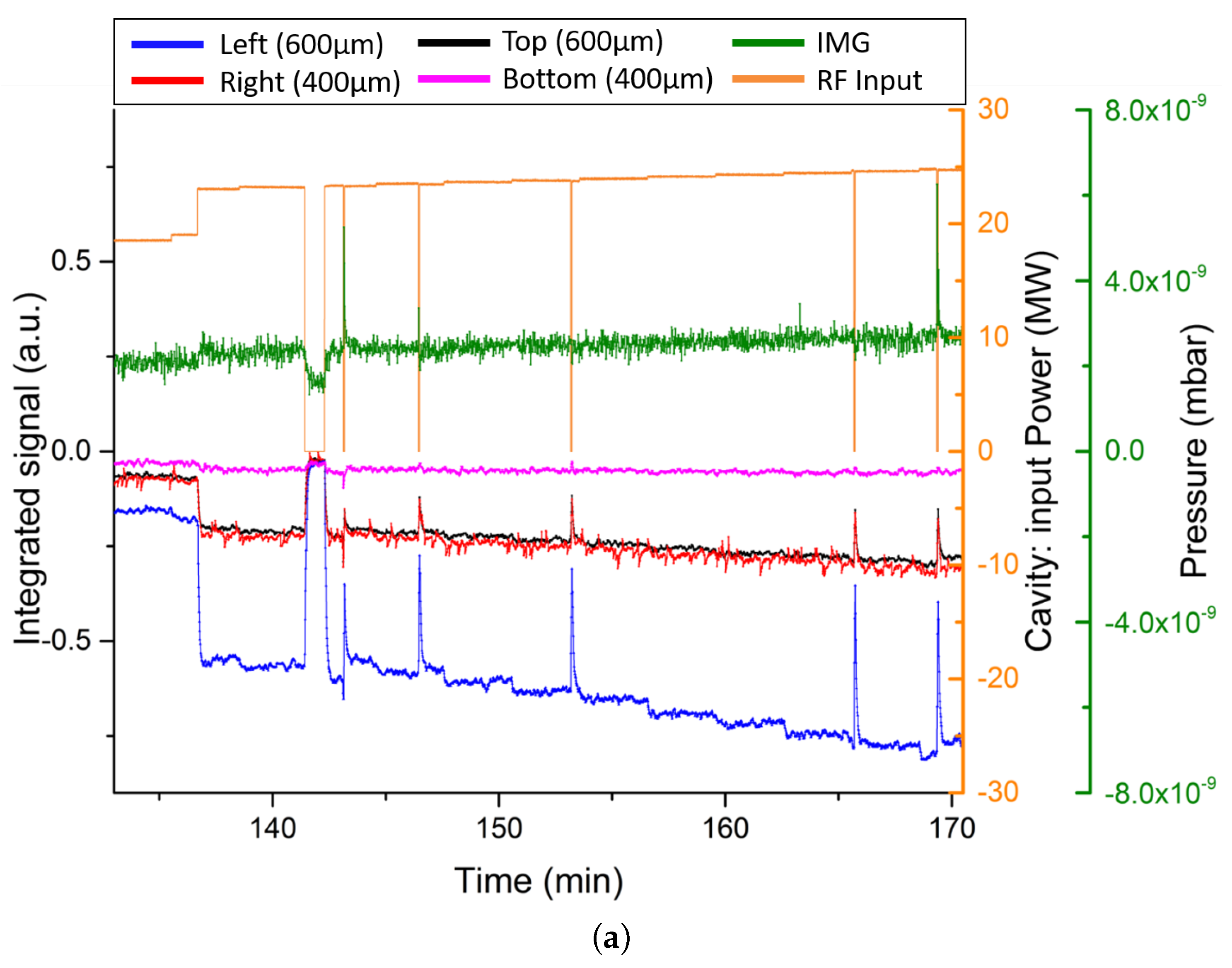
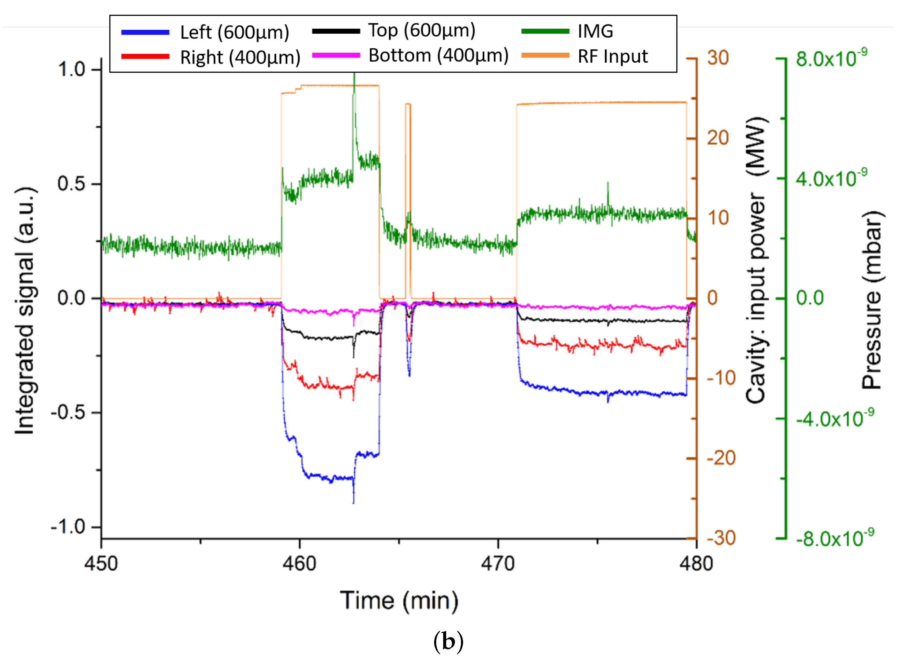
3.2. RF Breakdown
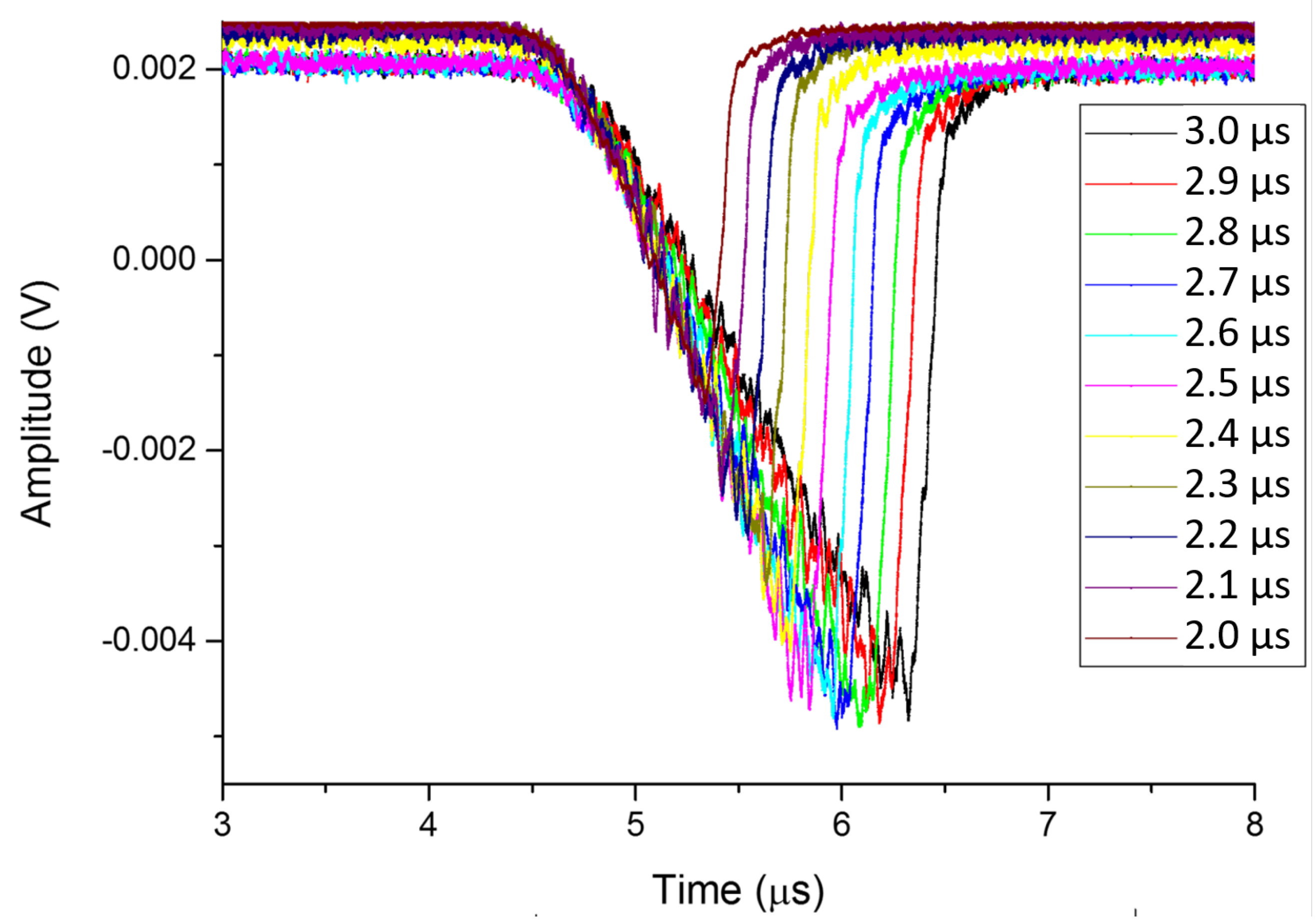
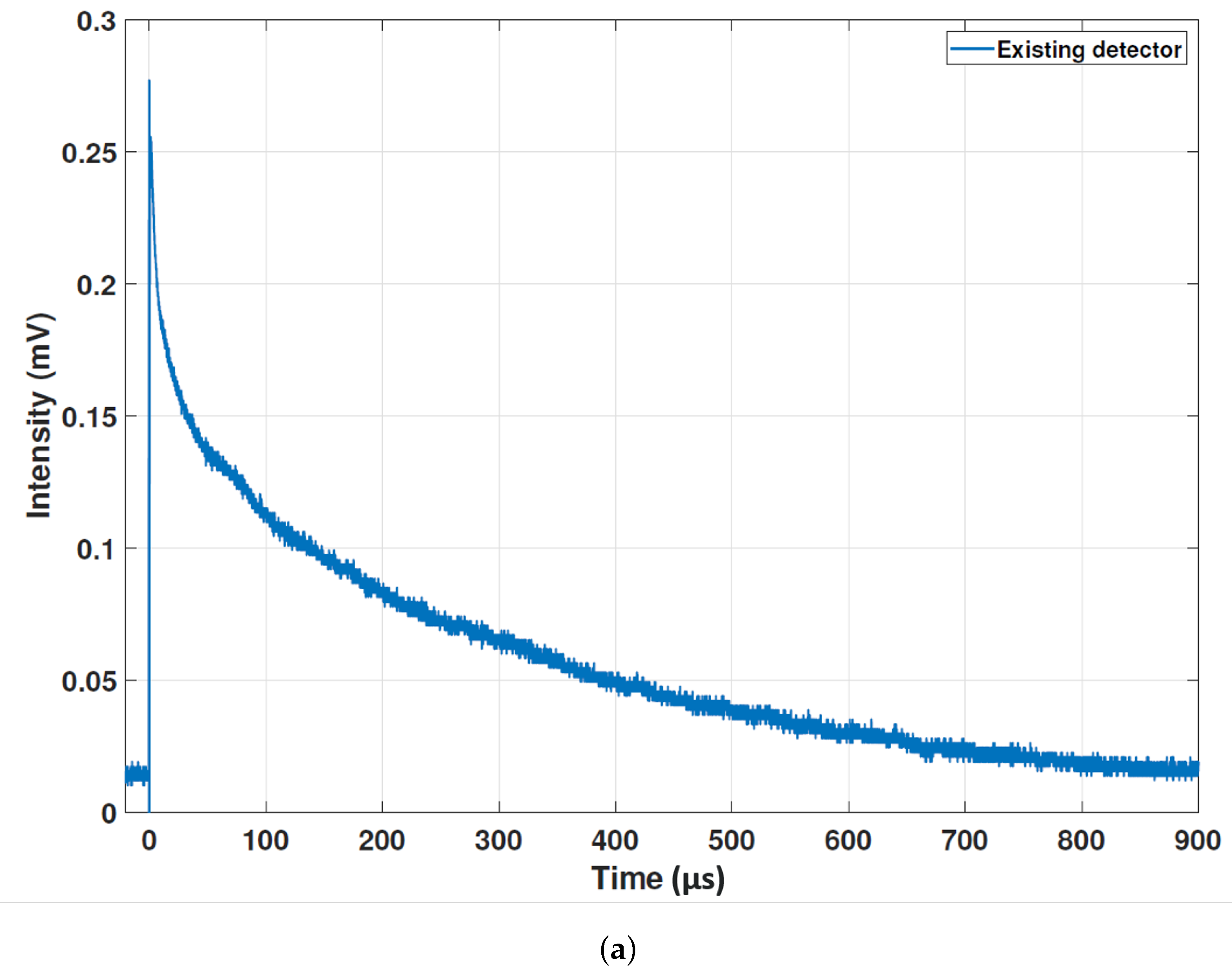
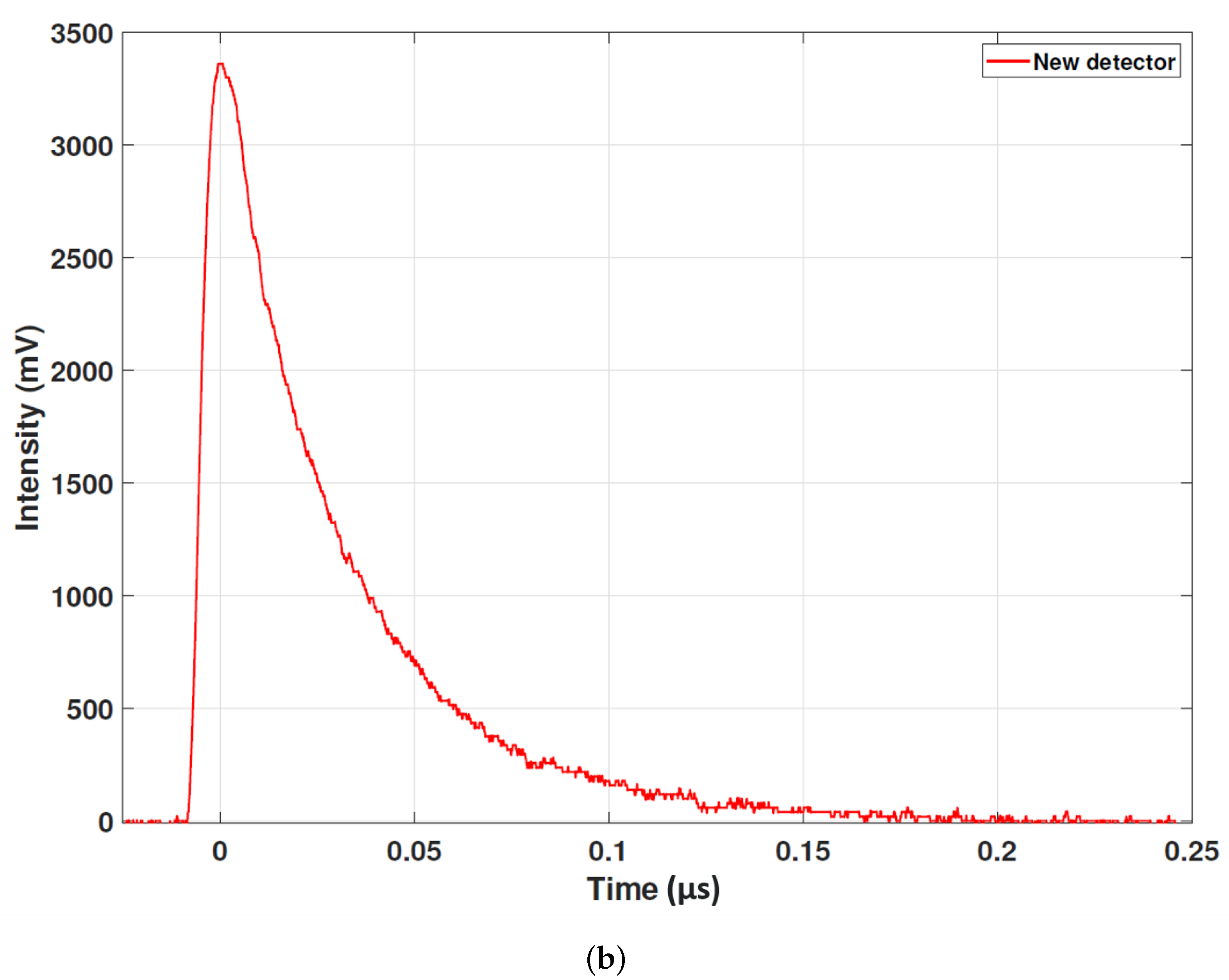
3.3. New System
4. Discussion
Author Contributions
Funding
Institutional Review Board Statement
Informed Consent Statement
Acknowledgments
Conflicts of Interest
References
- Maestre, J.; Torregrosa, C.; Kershaw, K.; Bracco, C.; Coiffet, T.; Ferrari, M.; Franqueira Ximenes, R.; Gilardoni, S.; Grenier, D.; Lechner, A.; et al. Design and behaviour of the Large Hadron Collider external beam dumps capable of receiving 539 MJ dump. J. Instrum. 2021, 16, P11019. [Google Scholar] [CrossRef]
- Angal-Kalinin, D.; Arduini, G.; Auchmann, B.; Bernauer, J.; Bogacz, A.; Bordry, F.; Bousson, S.; Bracco, C.; Brüning, O.; Calaga, R.; et al. PERLE. Powerful energy recovery linac for experiments. Conceptual design report. J. Phys. G Nucl. Part. Phys. 2018, 45, 065003. [Google Scholar] [CrossRef] [Green Version]
- Belousov, A.; Mustafin, E.; Ensinger, W. CCD based beam loss monitor for ion accelerators. Nucl. Instrum. Methods Phys. Res. A 2014, 743, 86–89. [Google Scholar] [CrossRef]
- Holzer, E.B.; Dehning, B.; Effnger, E.; Emery, J.; Grishin, V.; Hajdu, C.; Jackson, S.; Kurfuerst, C.; Marsili, A.; Misiowiec, M.; et al. Beam Loss Monitoring for LHC Machine Protection. Phys. Procedia 2012, 37, 2055–2062. [Google Scholar] [CrossRef] [Green Version]
- Andersson, R.; Nordt, A.; Bargalló, E.; Adli, E. Machine protection systems and their impact on beam availability and accelerator reliability. In Proceedings of the International Particle Accelerator Conference 2015, Richmond, VA, USA, 3–8 May 2015; p. MOPTY044. [Google Scholar]
- Yang, T.; Tian, J.; Zeng, L.; Xu, T.; Huang, W.; Sun, J.; Li, F.; Qiu, R.; Xu, Z.; Meng, M.; et al. Experimental studies and Monte Carlo simulations for beam loss monitors. Phys. Rev. Accel. Beams 2021, 24, 032804. [Google Scholar] [CrossRef]
- Stockner, M.; Dehning, B.; Fabjan, C.; Ferioli, G.; Holzer, E.B. Measurements and Simulations of Ionization Chamber Signals in Mixed Radiation Fields for the LHC BLM System. In Proceedings of the 2006 IEEE Nuclear Science Symposium Conference Record, San Diego, CA, USA, 29 October–1 November 2006; Volume 3, pp. 1342–1345. [Google Scholar]
- Wangler, T.P. Microwave Topics for Linacs. In RF Linear Accelerators; John Wiley & Sons: Hoboken, NJ, USA, 2008; pp. 156–164. [Google Scholar]
- Chen, Q.; Hu, T.; Qin, B.; Xiong, Y.; Fan, K.; Pei, Y. RF Conditioning Furthermore, Breakdown Analysis of a Traveling Wave Linac With Collinear Load Cells. Phys. Rev. Accel. Beams 2018, 21, 042003. [Google Scholar] [CrossRef] [Green Version]
- Pollard, A.; Gilfellon, A.J.; Dunning, D. Machine learning for RF breakdown detection at CLARA. In Proceedings of the Linear Acceleration Conference 2022, Liverpool, UK, 28 August–2 September 2017; p. WEPV021. [Google Scholar]
- Obermair, C.; Cartier-Michaud, T.; Apollonio, A.; Millar, W.; Felsberger, L.; Fischl, L.; Bovbjerg, H.S.; Wollmann, D.; Wuensch, W.; Catalan-Lasheras, N.; et al. Explainable machine learning for breakdown prediction in high gradient rf cavities. Phys. Rev. Acc. Beams 2022, 25, 104601. [Google Scholar] [CrossRef]
- Pimpec, F.L. Limitations on the Use of Acoustic Sensors in RF Breakdown Localization; Technical Report SLAC-TN-04-049 LCC-0149; SLAC National Accelerator Laboratory: Menlo Park, PA, USA, 2004. [Google Scholar]
- Geng, R.L.; Freyberger, A.; Legg, R.; Suleiman, R.; Fisher, A.S. Field Emission In SRF Accelerators: Instrumented Measurements For Its Understanding. In Proceedings of the International Beam Instrumentation Conference 2017, Grand Rapids, MI, USA, 20–24 August 2017; p. TH1AB1. [Google Scholar]
- Marchevsky, M. Protection of Superconducting Magnet Circuits; US Particle Accelerator School: Lisle, IL, USA, 2017.
- Kastriotou, M.; Holzer, E.B.; Nebot del Busto, E.; Welsch, C.P.; Bowland, M. An Optical Fibre BLM System at the Australian Synchrotron Light Source. In Proceedings of the International Beam Instrumentation Conference 2016, Barcelona, Spain, 11–15 September 2016; p. WEPG20. [Google Scholar]
- Kastriotou, M. Optimisation of Storage Rings and RF Accelerators via Advanced Fibre-Based Detectors. Ph.D. Thesis, University of Liverpool, Liverpool, UK, 2 May 2018. [Google Scholar]
- Alexandrova, A.S.; Devlin, L.; Tzoganis, V.; Welsch, C.P.; Brynes, A.; Jackson, F.; Effinger, E.; Holzer, E.B. Optical Beam Loss Monitors Based on Fibres for the CLARA Phase 1 Beam-Line. In Proceedings of the International Particle Accelerator Conference 2018, Vancouver, BC, Canada, 29 April–4 May 2018; p. THPML090. [Google Scholar]
- Giansiracusa, P.; Bowland, M.; Holzer, E.B.; Kastriotou, M.; LeBlanc, G.S.; Lucas, T.G.; Nebot del Busto, E.; Rassool, R.P.; Volpi, M.; Welsch, C.P. A distributed beam loss monitor for the Australian Synchrotron. Nucl. Instrum. Methods Phys. Res. A 2019, 919, 98–104. [Google Scholar] [CrossRef]
- Frank, I.; Tamm, I. Coherent visible radiation of fast electraons passing through matter. Comp. Rend. Dokl. Akad. Mauk. SSSR 1937, 14, 109–114. [Google Scholar]
- Benítez, S.; Salvachúa, B.; Chen, M.; Effinger, E.; Esteban, J.C.; Farabolini, W.; Korysko, P.; Lernevall, A.T. Beam Loss Localisation with an Optical Beam Loss Monitor in the CLEAR Facility at CERN. In Proceedings of the International Particle Accelerator Conference 2022, Bangkok, Thailand, 12–17 June 2022; p. MOPOPT045. [Google Scholar]
- Gundacker, S.; Heering, A. The silicon photomultiplier: Fundamentals and applications of a modern solid-state photon detector. Phys. Med. Biol. 2019, 65, 17TR01. [Google Scholar] [CrossRef] [PubMed]
- Multi-Photon Pixel Counter (MPPC) Manufactured by Hamamatsu Photonics K.K. Available online: https://www.hamamatsu.com/eu/en/product/optical-sensors/mppc/mppc_mppc-array.html (accessed on 27 November 2022).
- Hamamatsu Photonics, K.K. Photomultiplier Tubes: Basics and Applications, 4th ed.; Hamamatsu Photonics: Tokyo, Japan, 2017. [Google Scholar]
- Fisher, A.S.; Brown, G.W.; Chin, E.P.; Clarke, C.I.; Cobau, W.G.; Frosio, T.; Jacobson, B.T.; Kadyrov, R.A.; Mock, J.A.; Park, J.; et al. Commissioning Beam-Loss Monitors for the Superconducting Upgrade to LCLS. In Proceedings of the International Beam Instrumentation Conference 2022, Kraków, Poland, 11–15 September 2022; p. TU2C3. [Google Scholar]
- Kastriotou, M.; Degiovanni, A.; Domingues Sousa, F.S.; Effinger, E.; Holzera, E.B.; Navarro Quirante, J.L.; del Busto, E.N.; Teckera, F.; Vigano, W.; Welsch, C.P.; et al. RF cavity induced sensitivity limitations on Beam Loss Monitors. Phys. Procedia 2015, 77, 21–28. [Google Scholar] [CrossRef]
- Alexandrova, A.S.; Nebot del Busto, E.; Devlin, L.; Kastriotou, M.; Tzoganis, V.; Welsch, C.P.; Brynes, A.; Jackson, F.; Scott, D.J.; Effinger, E.; et al. Optical Beam Loss Monitor for RF Cavity Characterisation. In Proceedings of the International Beam Instrumentation Conference 2017, Grand Rapids, MI, USA, 20–24 August 2017; p. WEPWC01. [Google Scholar]
- Tennant, C.; Carpenter, A.; Powers, T.; Vidyaratne, L.; Iftekharuddin, K.; Monibor Rahman, M.; Shabalina, A. Superconductig Radio-Frequency Cavity Fault Classification using Machine Learning at Jefferson Laboratory. In Proceedings of the International Particle Accelerator Conference 2021, Campinas, Brazil, 24–28 May 2021; p. FRXC01. [Google Scholar]
- Imbasciati, L. Studies of Quench Protection in Nb3Sn Superconducting Magnets for Future Particle Accelerators. Ph.D. Thesis, Vienna Technical University, Vienna, Austria, 25 June 2003. [Google Scholar]
- Auchmann, B.; Baer, T.; Bednarek, M.; Bellodi, G.; Bracco, C.; Bruce, R.; Cerutti, F.; Chetvertkova, V.; Dehning, B.; Granieri, P.P.; et al. Testing beam-induced quench levels of LHC superconducting magnets. Phys. Rev. Spec. Top. Accel. Beams 2015, 18, 061002. [Google Scholar] [CrossRef]
- Bainbridge, A.R.; Angal-Kalinin, D.; Jones, J.K.; Pacey, T.H.; Saveliev, Y.M.; Snedden, E.W. The Design of the Full Energy Beam Exploitation (FEBE) Beamline on CLARA. In Proceedings of the International Particle Accelerator Conference 2022, Bangkok, Thailand, 12–17 June 2022; p. THPOPT015. [Google Scholar]
- D-Beam Ltd. Available online: www.d-beam.co.uk (accessed on 27 November 2022).
- J-Series SiPM Manufactured by Semiconductor Components Industries, LLC. Available online: https://www.onsemi.com/products/sensors/photodetectors-sipm-spad/silicon-photomultipliers-sipm (accessed on 27 November 2022).


Disclaimer/Publisher’s Note: The statements, opinions and data contained in all publications are solely those of the individual author(s) and contributor(s) and not of MDPI and/or the editor(s). MDPI and/or the editor(s) disclaim responsibility for any injury to people or property resulting from any ideas, methods, instructions or products referred to in the content. |
© 2023 by the authors. Licensee MDPI, Basel, Switzerland. This article is an open access article distributed under the terms and conditions of the Creative Commons Attribution (CC BY) license (https://creativecommons.org/licenses/by/4.0/).
Share and Cite
Wolfenden, J.; Alexandrova, A.S.; Jackson, F.; Mathisen, S.; Morris, G.; Pacey, T.H.; Kumar, N.; Yadav, M.; Jones, A.; Welsch, C.P. Cherenkov Radiation in Optical Fibres as a Versatile Machine Protection System in Particle Accelerators. Sensors 2023, 23, 2248. https://0-doi-org.brum.beds.ac.uk/10.3390/s23042248
Wolfenden J, Alexandrova AS, Jackson F, Mathisen S, Morris G, Pacey TH, Kumar N, Yadav M, Jones A, Welsch CP. Cherenkov Radiation in Optical Fibres as a Versatile Machine Protection System in Particle Accelerators. Sensors. 2023; 23(4):2248. https://0-doi-org.brum.beds.ac.uk/10.3390/s23042248
Chicago/Turabian StyleWolfenden, Joseph, Alexandra S. Alexandrova, Frank Jackson, Storm Mathisen, Geoffrey Morris, Thomas H. Pacey, Narender Kumar, Monika Yadav, Angus Jones, and Carsten P. Welsch. 2023. "Cherenkov Radiation in Optical Fibres as a Versatile Machine Protection System in Particle Accelerators" Sensors 23, no. 4: 2248. https://0-doi-org.brum.beds.ac.uk/10.3390/s23042248