

Net Isotopic Signature of Atmospheric CO2 Sources and Sinks: No Change since the Little Ice Age


Department of Water Resources and Environmental Engineering, School of Civil Engineering, National Technical University of Athens, Heroon Polytechneiou 5, 157 72 Zographou, Greece
Sci 2024, 6(1), 17; https://0-doi-org.brum.beds.ac.uk/10.3390/sci6010017
Submission received: 19 December 2023
/
Revised: 23 February 2024
/
Accepted: 29 February 2024
/
Published: 14 March 2024
(This article belongs to the Special Issue Feature Papers—Multidisciplinary Sciences 2023)
Abstract
:Recent studies have provided evidence, based on analyses of instrumental measurements of the last seven decades, for a unidirectional, potentially causal link between temperature as the cause and carbon dioxide concentration ([CO2]) as the effect. In the most recent study, this finding was supported by analysing the carbon cycle and showing that the natural [CO2] changes due to temperature rise are far larger (by a factor > 3) than human emissions, while the latter are no larger than 4% of the total. Here, we provide additional support for these findings by examining the signatures of the stable carbon isotopes, 12 and 13. Examining isotopic data in four important observation sites, we show that the standard metric δ13C is consistent with an input isotopic signature that is stable over the entire period of observations (>40 years), i.e., not affected by increases in human CO2 emissions. In addition, proxy data covering the period after 1500 AD also show stable behaviour. These findings confirm the major role of the biosphere in the carbon cycle and a non-discernible signature of humans.
| We own the science, and we think that the world should know it. |
| Melissa Fleming, Under-Secretary-General for Global Communications at the United Nations during the 2022 World Economic Forum’s Sustainable Development Impact Meetings [1] |
1. Introduction
In their recent studies, Koutsoyiannis and Kundzewicz [2] questioned the conventional wisdom that increased atmospheric carbon dioxide concentration ([CO2]) causes increase in temperature (T) and Koutsoyiannis et al. [3,4,5] provided evidence, based on analyses of instrumental measurements of the last seven decades, for a unidirectional, potentially causal link between T as the cause and [CO2] as the effect. The latest of these studies [5], supported this finding by analysing the carbon cycle and showing that the natural [CO2] changes due to temperature rise in the last 65 years are far larger (by a factor > 3) than human emissions, while the latter are no larger than 4% of the total.
The latter study raised wide interest and was subsequently discussed in several forums, among which the most representative is Judith Curry’s blog [6]. With its approximately 1000 comments, 18% of which were replies by the principal author, this extended discussion, equivalent in length to a book of 370 pages [7], can be regarded as an interesting case of post-publication crowd reviewing, which the study withstood. Some of the comments tried to refute the findings of the paper by invoking arguments related to changes in the isotopic composition of atmospheric CO2, and particularly in the signatures of the stable carbon isotopes, 12 and 13, as expressed by the standard metric δ13C in CO2, defined below. These could not be replied to with arguments contained in this paper as the issues are out of its scope. At the same time, the comments triggered the present study to investigate the issue. By investigating modern instrumental data of δ13C and [CO2], as well as proxy data for older periods, starting from the Little Ice Age (early-16th century, to mid-19th century) we try to answer the following research questions:
- Do modern instrumental carbon isotopic data, available for a period of observations of more than 40 years, reflect changes due to human (fossil fuel) CO2 emissions?
- Does the modern period differ, in terms of the net isotopic signature of atmospheric CO2 sources and sinks, from earlier periods since the Little Ice Age?
The stable carbon isotopes 12C and 13C are present in the atmosphere, the oceans, and the terrestrial biosphere in percentages of 99% and 1%, respectively [8]. Slight variations in these percentages depend on biochemical processes, volcanic activity, and atmospheric and oceanic processes, while lately, human activities have also been regarded as agents of such variations. Carbon also appears in the unstable isotopic form 14C, but in trace amounts (of the order of 1 × 10⁻¹²). In the 1950s and 1960s, its presence was dramatically increased due to nuclear weapons testing, which produced 14C in the atmosphere. Subsequently, its concentration in the atmosphere has been dropping. Due to its complicated dynamics, driven mostly by nuclear reactions and decay, 14C will not be considered in this study, whose scope is the change in the stable isotopes 12C and 13C.
Based on these two isotopes, we define the basic quantity used throughout this paper as follows:
Definition 1.
The isotopic signature related to the stable carbon isotopes 12C and 13C, is
with the subscript “s” denoting an established standard reference material.
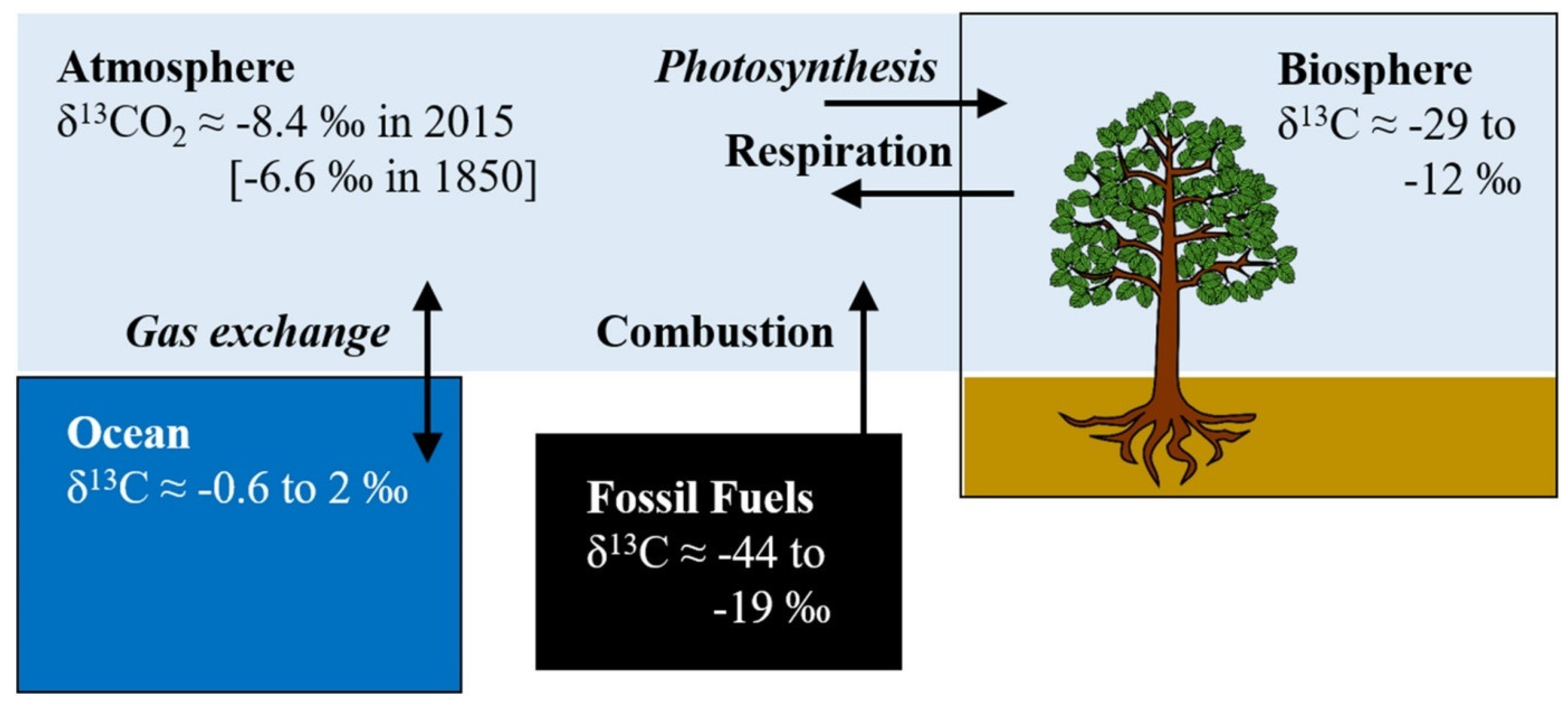
This is also known as reduced isotopic ratio and is typically reported in parts per thousand (per mil, ‰). The standard reference material is the Vienna Pee Dee Belemnite (PDB) limestone [9,10]. The transformation of Equation (1) makes the slight natural variations of appear with familiar values, as seen in Figure 1, which shows that different compartments of the climate system and Earth have different isotopic signatures. The figure also shows that some of the processes perform a function known as fractionation, that is, isotope discrimination. In particular, photosynthesis, during the exchange of O2 and CO2, discriminates against the heavier isotope 13C and, as a result, the isotope is generally depleted in plants.
In recent years, a decrease in atmospheric δ13C has been observed, which is often termed the Suess Effect after Suess (1955) [11], who published the first observations on this phenomenon on trees, albeit using 14C data. He attributed the decrease to human activities, stating:
The decrease [in the specific 14C activity of wood at time of growth during the past 50 years] can be attributed to the introduction of a certain amount of C14-free CO2 into the atmosphere by artificial coal and oil combustion and to the rate of isotopic exchange between atmospheric CO2 and the bicarbonate dissolved in the oceans.
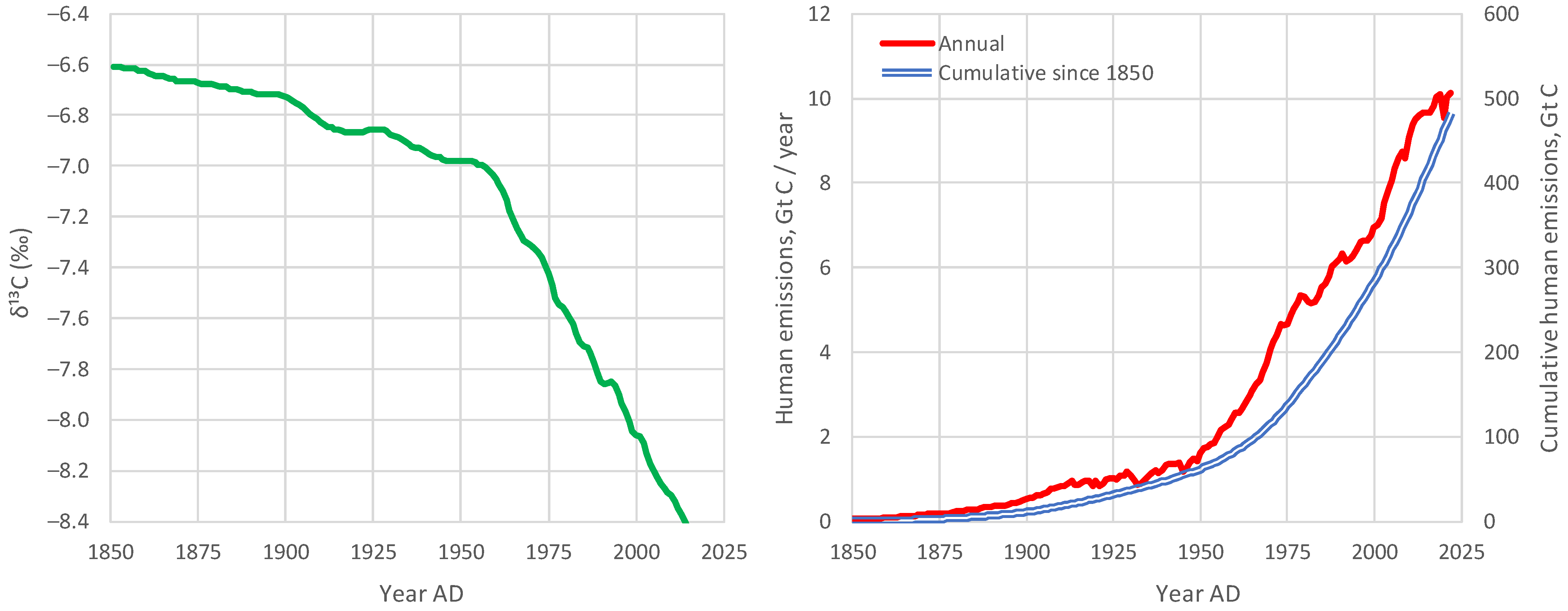
There is no question that δ13C has been decreasing and that human emissions have been increasing since the Industrial Revolution (Figure 2). Also, as seen in Figure 1, the combustion of fossil fuels can have an effect on reducing δ13C, as they are relatively depleted in 13C. This was the line of thought behind Suess [11] (even though the above quotation refers to 14C) and has become a common conviction thereafter.
The carbon isotopic (δ13C, PDB) signature of fossil fuel emissions has decreased during the last century, reflecting the changing mix of fossil fuels produced.
Also, in their recent review paper, Graven et al. [8] noted:
Carbon isotopes, 14C and 13C, in atmospheric CO2 are changing in response to fossil fuel emissions and other human activities.[…]Emissions of CO2 from fossil fuel combustion and land use change reduce the ratio of 13C/12C in atmospheric CO2 (δ13CO2). This is because 12C is preferentially assimilated during photosynthesis and δ13C in plant-derived carbon in terrestrial ecosystems and fossil fuels is lower than atmospheric δ13CO2.[…]Cement manufacturing also involves “fossil” carbon in that the source material is geological and therefore free of any 14C.[…]Since the Industrial Revolution, the carbon isotopic composition of atmospheric CO2 has undergone dramatic changes as a result of human activities and the response of the natural carbon cycle to them. The relative amount of atmospheric 14C and 13C in CO2 has decreased because of the addition of 14C- and 13C-depleted fossil carbon.
These generally accepted hypotheses, however, may reflect a dogmatic approach, or a postmodern ideological effect, i.e., to blame everything on human actions. Hence, the null hypothesis that all observed changes are (mostly) natural has not seriously been investigated. However, there are good reasons for this investigation. It is a fact that the biosphere has become more productive and expanded [5,17,18,19], resulting in natural amplification of the carbon cycle due to increased temperature. This fact may have been a primary factor for the decrease in the isotopic signature δ13C in atmospheric CO2. Note that the emissions of the biosphere are much larger than fossil fuel emissions (where the latter are only 4% of the total) [5] and, as seen in Figure 1, the biosphere’s isotopic signature δ13C is much lower than the atmospheric (see also Section 6).
In addition to the biosphere’s action, other natural factors also affect the input isotopic signature in the atmospheric CO2. These include volcano eruptions, among which, in the recent period, the Pinatubo eruption in 1991 is regarded as the most important, as well as the interannual variability related to El Niño—Southern Oscillation (ENSO) [8].
To investigate the null hypothesis and answer the two research questions posed above, we use modern instrumental and proxy data, as described in Section 2. We develop a theoretical framework in Section 3, which we apply to the data in a diagnostic mode in Section 4, and in a modelling mode in Section 5. The findings of these applications are further discussed in Section 6 and the conclusions are drawn in Section 7.
2. Data
Systematic measurements of the isotopic signature in atmospheric CO2 have been made since 1978 [20] by the Scripps CO2 Program of the Scripps Institution of Oceanography, University of California, and are available online [21,22,23]. The data include observations of CO2 concentration (in micro-moles CO2 per mole, or parts per million—ppm), as well as observations (in ‰). The latter are made at an irregular frequency, which varies between once every 4–5 days to once every 15–30 days, depending on the time period and the site (where the ranges are given for 95% of frequencies). These raw data are then processed to extract monthly values, filled in in case of missing data. In addition to the actual monthly values, the Scripps CO2 Program provides seasonally adjusted values, in which the seasonal variation is purportedly removed. All available time series—daily, monthly, and seasonally adjusted monthly—have been retrieved and processed here. Among the available observation sites, the four most important were chosen, which are shown in Table 1, along with their characteristics.
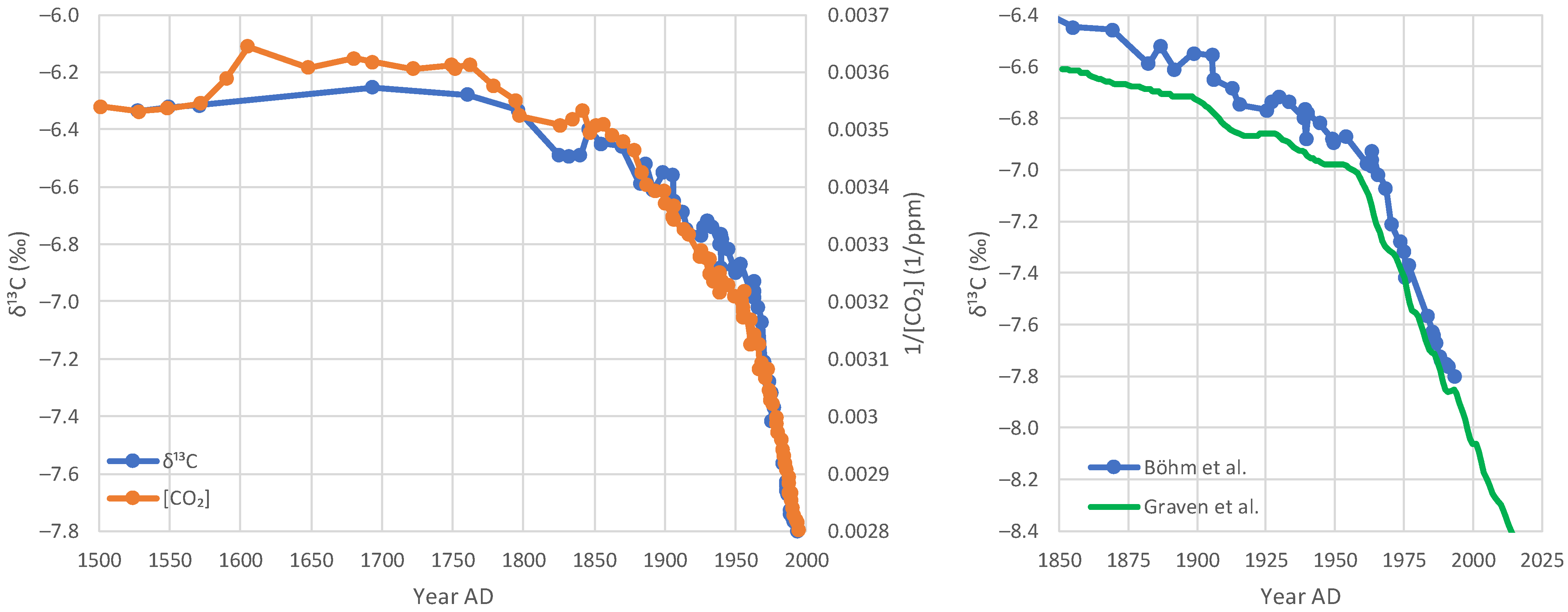
In addition to the instrumental data, proxy data for the last five centuries were analysed in this study. These were retrieved by digitisation of Figure 4 of Böhm et al. [24], a study that used carbon isotope records of four Caribbean coralline sponges to derive records, combined with an ice core record. Here, the atmospheric data of [CO2] and from that study are used. These were derived from Antarctic ice core, firn air inclusions and air measurements, while the atmospheric record was scaled for its preindustrial mean and minimum values to fit the shallow water sponge record. The two digitised series are shown in the left panel of Figure 3, where the right panel, which compares this data set with that of Graven et al. [8] (also seen in Figure 2) is indicative of the uncertainty in the proxy information.
3. Theoretical Framework
We assume that in a container of a gas mixture of total mass m, a particular gas A appears at concentration C. To the container, we inject an elementary (differential) mass dm, in which A appears at input concentration . Mass conservation results in:
This results in an ordinary first-order linear differential equation:
where, for generality, we assume that both and vary with m (and hence are functions of m).
It is stressed that the input in Equation (2) is not necessarily provided by a single source. It could be the result of n sources and sinks:
where is the proportion, in terms of mass input, of source (or sink) i over the total, satisfying:
and is the concentration of gas A in source i. Then, the input concentration is defined as
In addition, the different need not necessarily be positive. Some of them could be negative, signifying mass removal (sink, instead of source, for which ).
The general solution of Equation (3), assuming initial condition and , is:
where is the average input concentration, i.e.,
In the special case that the input concentration is constant, Equation (7) can be written as:
There is a linear relationship between and , which can be utilised to find from the data of and . For varying we may find the average over a period in which the mass varies from an initial value to a final value as:
In order to apply these relationships on the isotopic characterisation of the atmospheric CO2, we assume that the container is the entire atmosphere. We observe that the mass of CO2 in the atmosphere is proportional to the concentration , typically expressed in volumetric parts per million (ppm), and the concentration of the fraction of the isotope 13C in CO2 is proportional to , where is the isotopic signature defined in Equation (1). Under these conditions, Equation (7), after algebraic manipulations, becomes:
where the subscript ‘I’ denotes input (source or sink), the subscript ‘0’ denotes initial condition and the overbar denotes average. Likewise, for the constant input isotopic signature , Equation (9) becomes:
For the constant input isotopic signature we can utilize Equation (12) to find as the intercept of a linear regression from data of and . Based on this we may proceed to the following:
Definition 2.
A Keeling plot is a plot of
vs. , where the values of and are simultaneous.
Apparently, this definition does not convey any new idea, but rather, the very name of the plot is a reminder of its first usage by Charles D. Keeling more than 60 years ago [25,26]. Keeling introduced it as a linear plot empirically, after exploration of data, while later, Miller and Tans [27], and Köhler et al. [28], introduced a theoretical justification of its linearity, as in Equation (12), based on mass balance.
We clarify here that, as implied by Definition 2, we use the term here irrespective of the linearity or not of the plot. The definition only describes the axes of the plot, while the linearity, whenever it appears, suggests an input isotopic signature invariable in time.
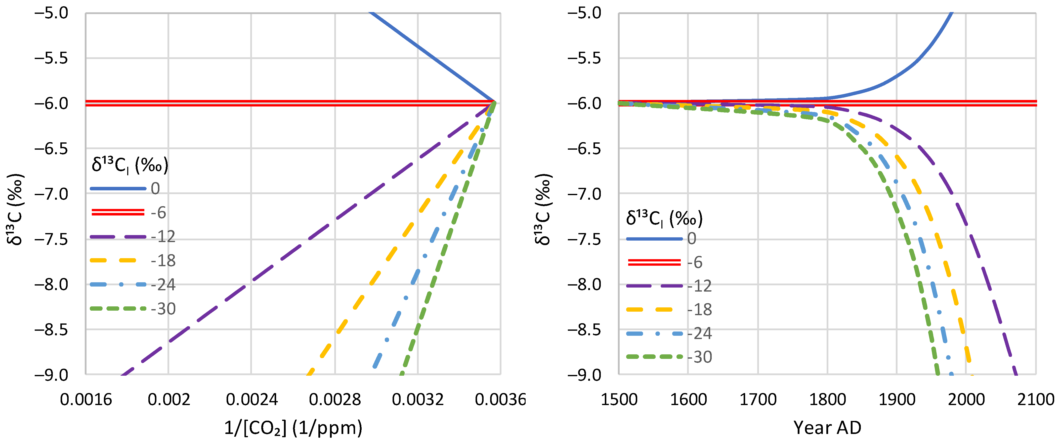
The Keeling plot is distinguished from a common time series plot, like those of Figure 3. While the former readily provides indication of the constancy of the input isotopic signature, the latter does not. This is illustrated in Figure 4, which shows both a Keeling plot and a time series plot. To make the plots, we assumed initial conditions that resemble those on Earth in 1500 AD and alternative input isotopic signatures , in all cases invariable in time, so that Equation (12) holds. (Additional information about the construction of Figure 4 is provided in its caption and Section 4 and Section 5). It is notable that in the time series plot (Figure 4, right panel), for low values of the input isotopic signature, curves appear that resemble those of the proxy data in Figure 3. Their curvature does not provide any indication that the input isotopic signature is actually constant, but the Keeling plot (Figure 4, left panel) readily reveals that constancy by the linearity of the plots.
In the case that the input isotopic signature is not constant, the Keeling plot will not be linear as in Equation (12). In this case, to find isotopic signatures as averages either globally (for the entire period of observations) or locally, over certain subperiods, it is preferable to use the following equation, which is a consequence of Equation (10):
Note that, from the form of the equation, only the initial and final conditions in the studied period matter in the calculation of . For numerical stability, the length of the subperiods should not be too short, so that the difference in the denominator be relatively large. An illustration is given in Section 4 where that difference is typically taken equal to the standard deviation of the observations.
Köhler et al. [28] claimed that there are two basic assumptions underlying the Keeling plot method: (1) The system consists of (only) two connected reservoirs; and (2) The isotopic ratio of the carbon in the added reservoir does not change during the time of observation. Here, we have removed both these assumptions, which are unnecessary in our general formulation. First, we do not consider two reservoirs, but one reservoir (e.g., the entire atmosphere) plus an input, which may lump many components, as in Equation (4). The removal of this assumption was absolutely necessary, as the final isotopic signature of atmospheric results from the mixing of processes of diverse sources. Second, the general solution of the differential equation (Equations (11) and (13)) is valid, even for the varying isotopic ratio of the carbon.
It is noted that in the case of a net sink instead of a net source (mass removal, instead of injection), the solution remains the same. If the net source or sink has a constant concentration, , then the average, calculated by the Equation (13) will also be constant, . However, if there are seasonal increasing and decreasing phases of with a constant isotopic signature in each phase that is different in the two phases, namely and for the phases that goes up and down, respectively, then the average which characterizes the over-year changes, is different from both and . Such a difference in the two phases can be expected due to fractionation in the biosphere, particularly that of photosynthesis (see Figure 1).
To find the long-term average in this case, we assume a system with initial conditions , which, within one time period, one year in the present case, undergoes increases and decreases in with a total increase and decrease and , and total change in the time period , so that the state in the end of the period is (). As shown in Appendix A, the average can be calculated by
where
Even a small difference between the seasonal may result in largely deviating over-year average , depending on that difference and the ratio . This is illustrated in Figure 5, where it is seen that a difference of ±5‰ between may easily result in differences of ±25‰ between those and the over-year average .
4. Diagnostic Results
4.1. Initial Observations
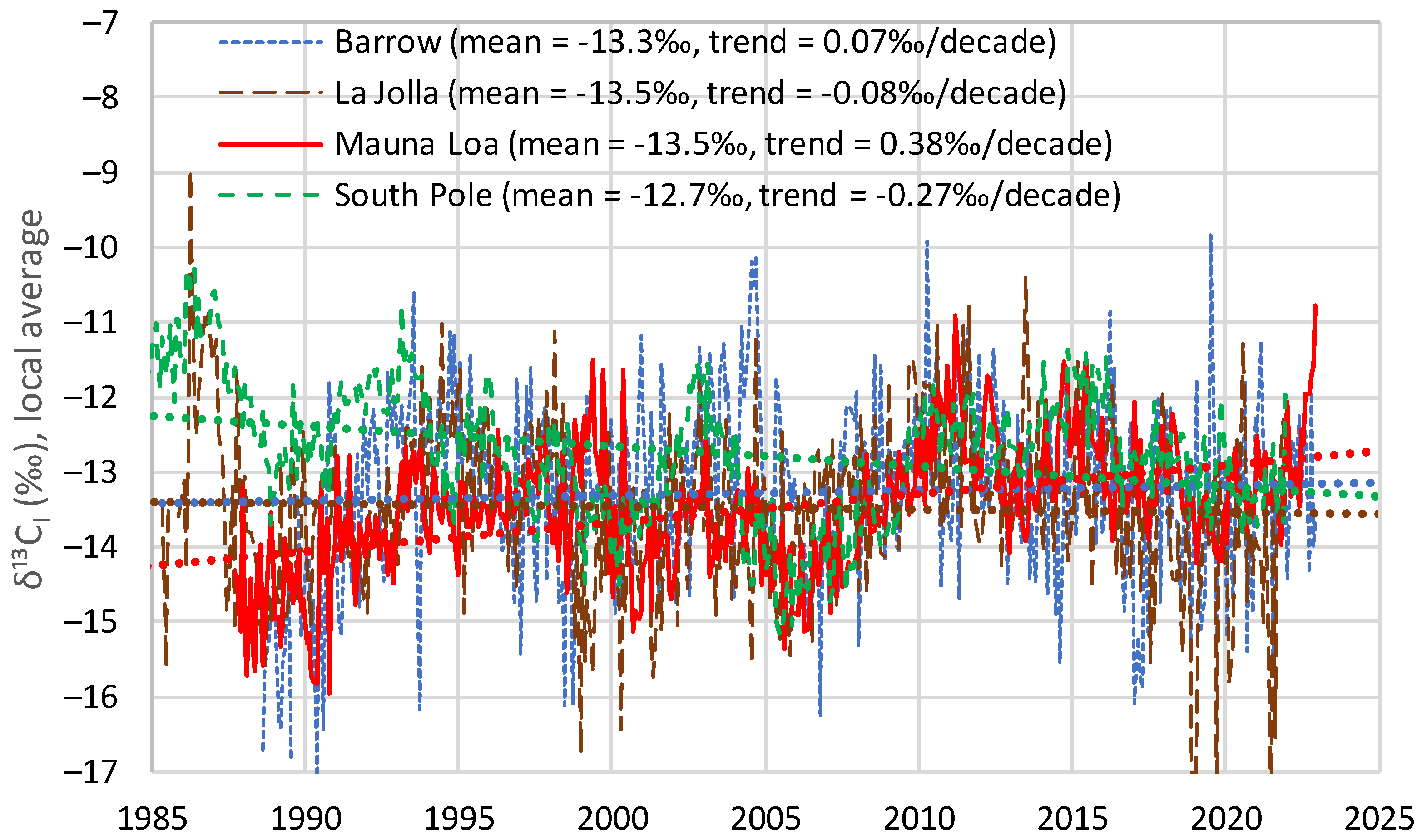
Figure 6 (upper panel) shows the four instrumental time series of in atmospheric in a monthly scale and allows us to make the following observations:
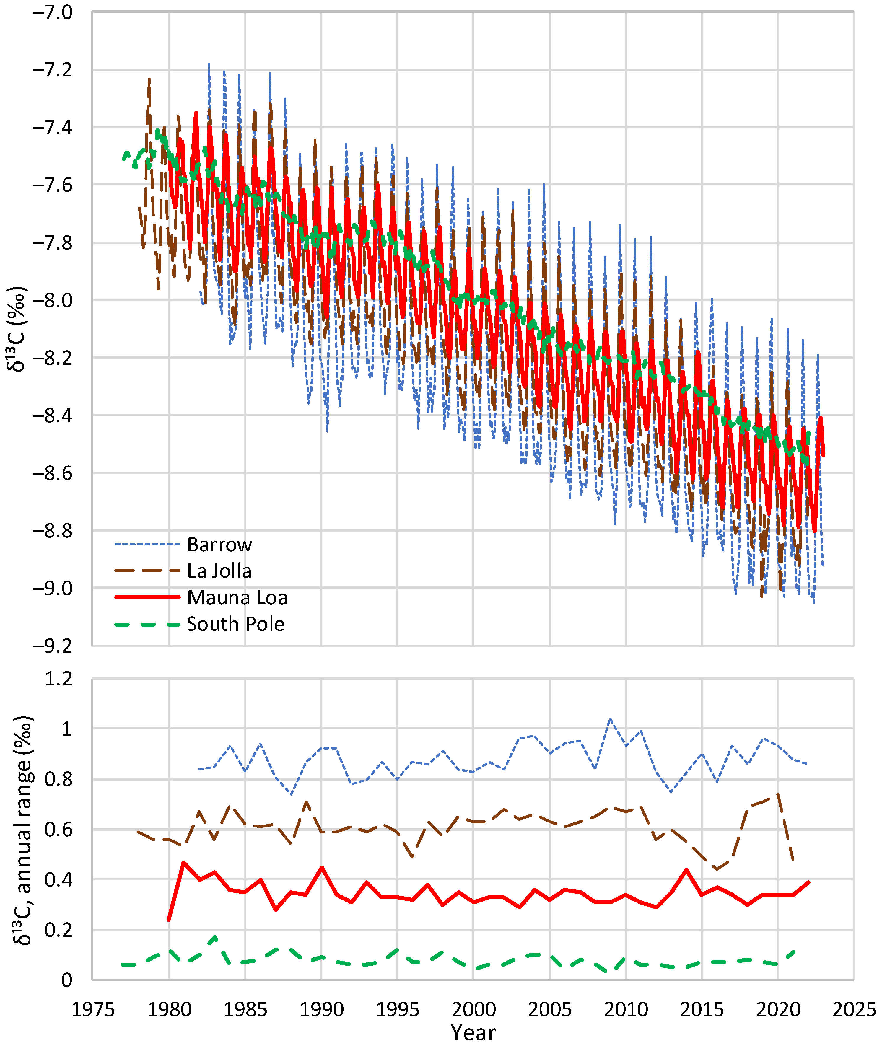
- All four series show a long-term tendency to decrease through the years;
- The time series of Barrow, which is the northernmost site, exhibits a substantial seasonal variation, with an annual range of variation of nearly 1‰, almost equal to the interannual central change through the entire period of observations;
- As we go from north to south, the seasonal variation is reduced and at the South Pole it is minimal;
- Apart from the seasonal variation, the behaviours of all series are similar, as indicated by the long-term slopes in the figure.
The pronounced seasonality, which is also depicted in the lower panel of Figure 6 in terms of the annual range (maximum minus minimum value per year for each of the four instrumental time series) is a clear sign of the domination of the biosphere processes, i.e., respiration and photosynthesis, in driving the isotopic signature . In particular, photosynthesis removes CO2 from the atmosphere and the fractionation that characterises it results in an increase in in the atmosphere, during the months it occurs. Furthermore, the decreasing intensity of seasonality as we move from north to south may be related to the fact that the majority of land lies in the northern hemisphere, which suggests a major role of the terrestrial biosphere in controlling the cycle of the isotopic signature (see also Section 6). It is also notable that no trend appears in the seasonal behaviour (lower panel of Figure 6). Considering the fact that, as seen in Figure 2 (right), the human carbon emissions per year have been doubled in the time period covered by Figure 6, if these were a key factor, this would somehow be reflected in a trend in the seasonality. Therefore, no sign is discerned that would necessitate an attribution to the influence of fossil fuel emissions. In contrast, Figure 6 suggests that the key processes in CO2 emissions are related to biosphere processes such as respiration and photosynthesis.
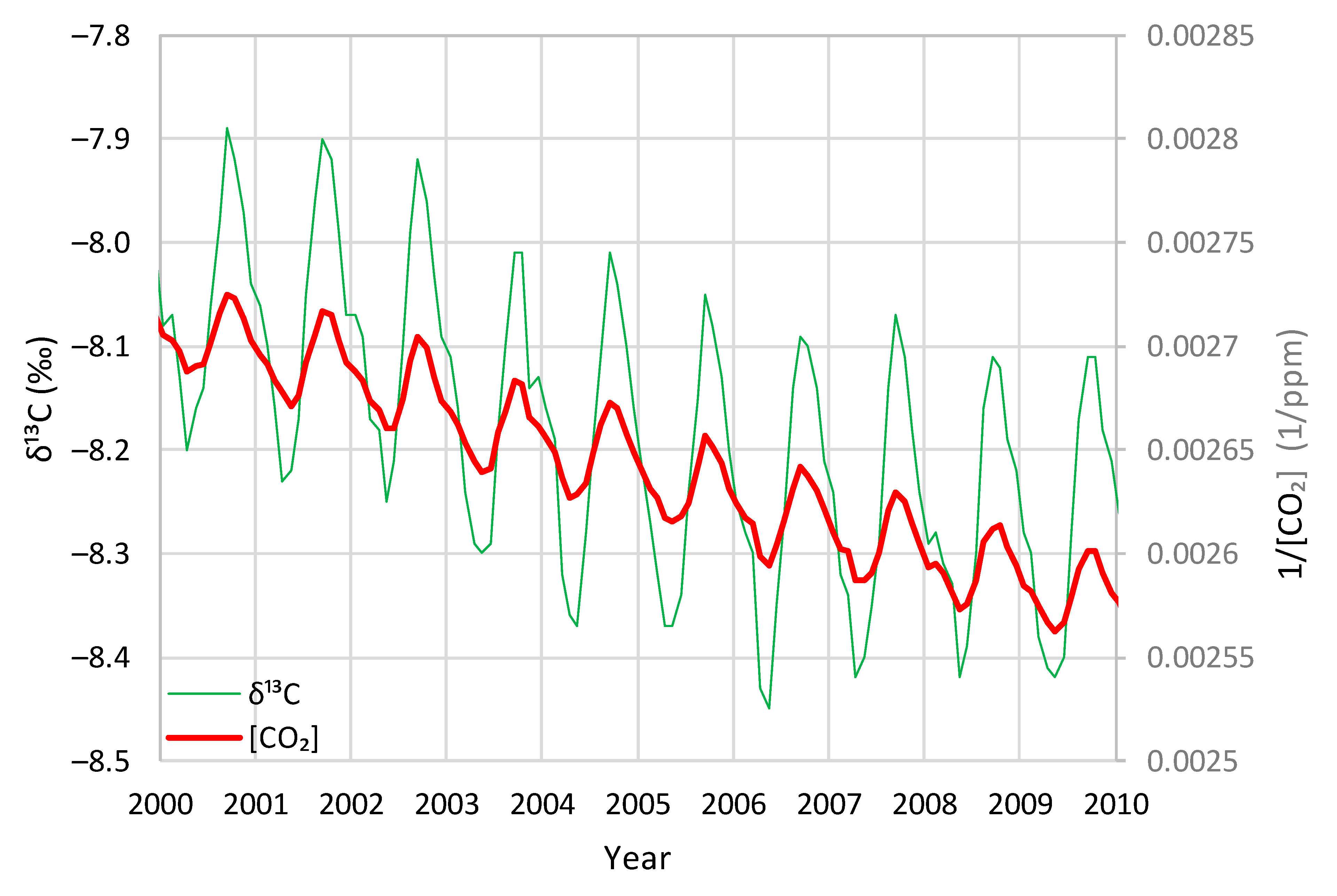
The seasonality effect that is maximal in Barrow, Alaska, continues to be present even in the tropics in the northern hemisphere. A depiction of the Mauna Loa site can be seen in Figure 7, which, for better legibility, focuses on one decade. In it, the inverse of the carbon dioxide concentration, , is also plotted. A perfect synchronisation of and changes is observed, which is justifiable by the theoretical considerations of Section 3. This raises the question as to whether adds any information to that already present in . We will investigate this further below.
4.2. Comparison of the Behaviours at Different Time Scales
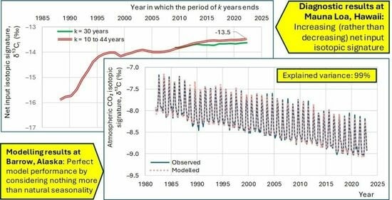
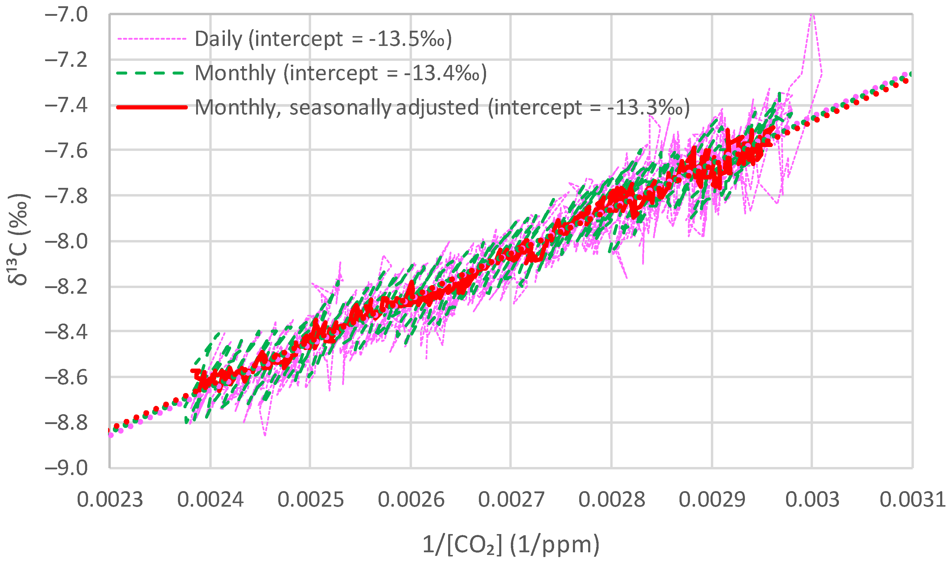
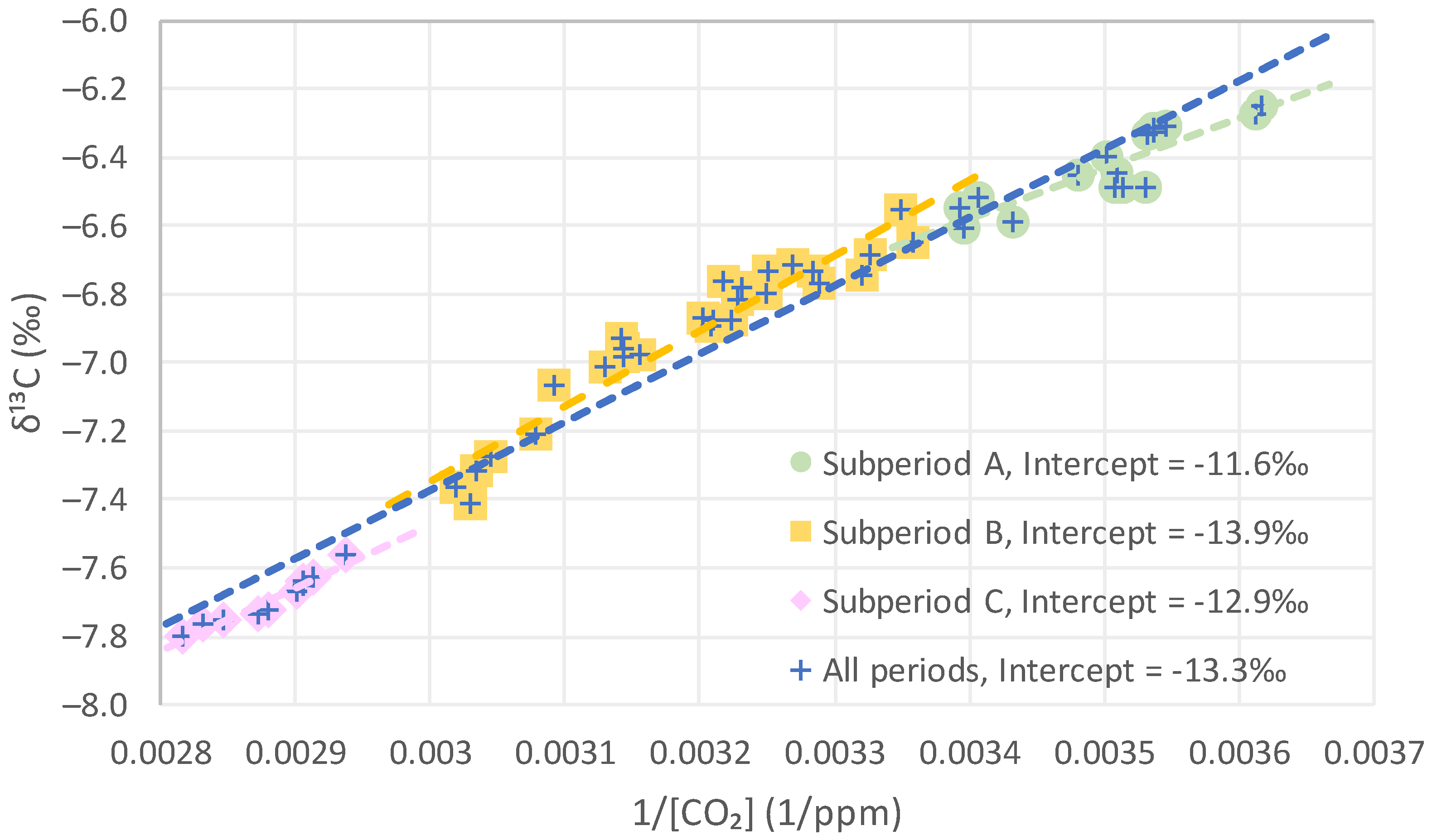
The Keeling plot, based on Equation (12) and described in Section 3, is a powerful diagnostic tool for the behaviour of the isotopic signature in the atmosphere. Figure 8 shows the Keeling plots for Mauna Loa for all three available time series, daily, monthly and seasonally adjusted.
The seasonally adjusted time series yields an almost perfect linear plot with a very high coefficient of determination, R2 = 0.99 and an intercept of −13.3‰, which represents an input isotopic signature , constant for the entire period of observations. However, the daily and monthly time series clearly show that the input signature is not constant, but is seasonally varying with higher slopes, locally corresponding to intercepts of about −25‰. Yet apart from the scatter due to seasonality, the plots make a linear arrangement with linear trend lines, also shown in the graph, with intercepts very close to −13.3‰.
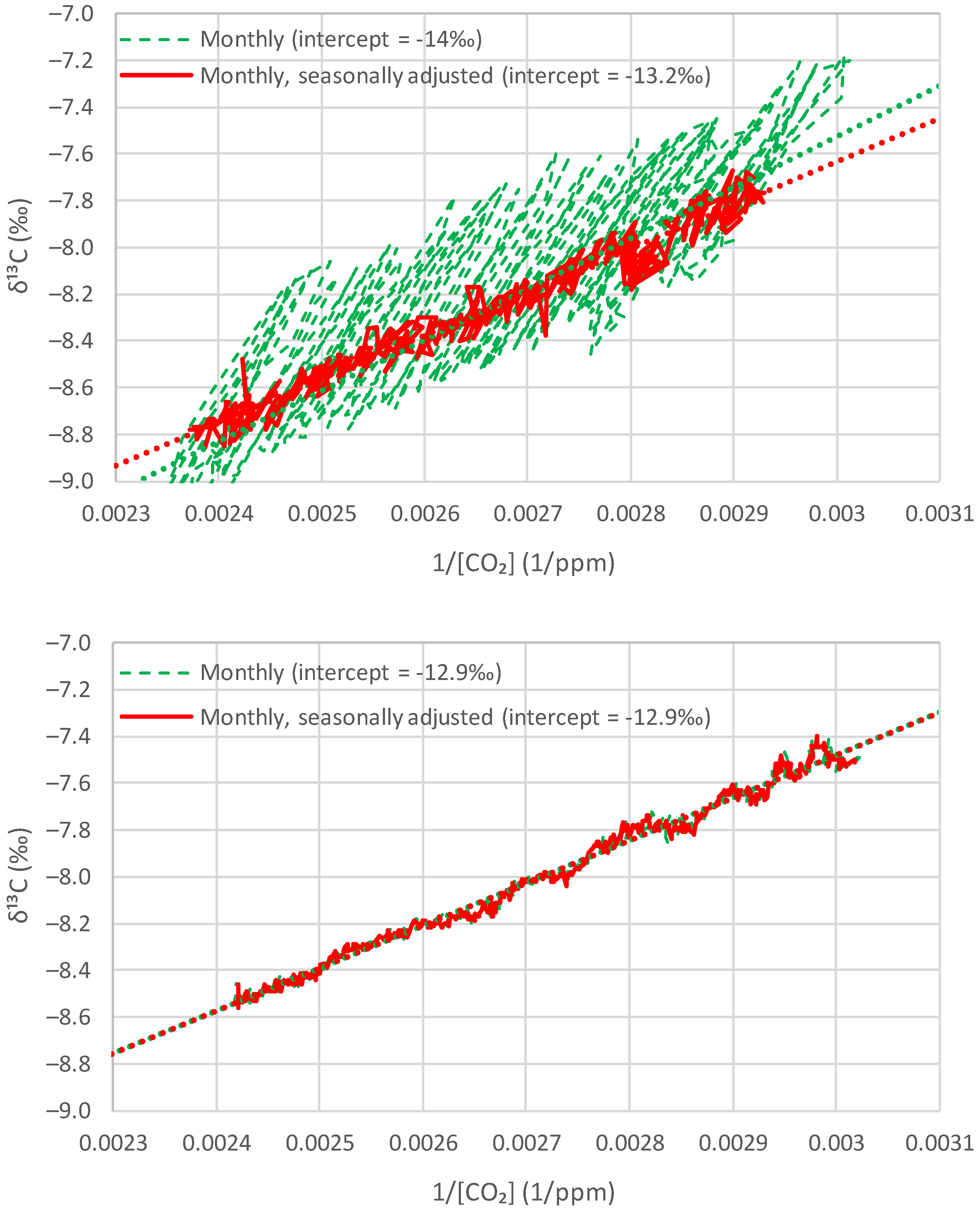
Figure 9 shows similar plots for Barrow and the South Pole. In the former, the seasonality is prominent and in the latter, it is almost absent. Yet the overall arrangements are linear, with intercepts between and , which are not very different from those in Figure 8.
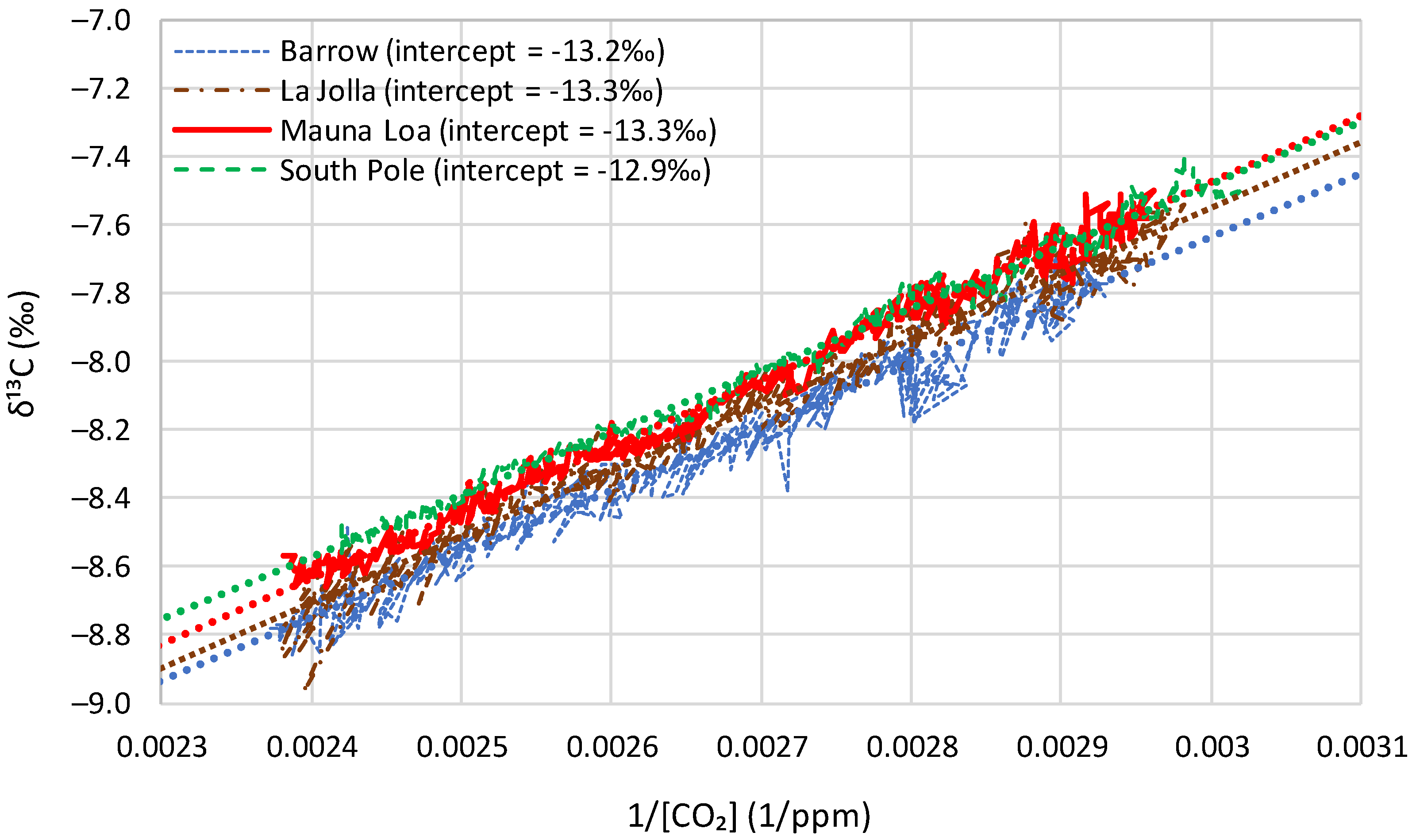
Figure 10 compares the Keeling plots of all four sites for the seasonally adjusted time series. The similarity is noticeable, and the intercepts are very close to each other, varying in the narrow range of to . In brief, the over-annual input isotopic signature is almost the same for the entire globe.
4.3. Investigation of Over-Year Changes
The graphical depictions of Section 4.2 do not suggest any long-term change in the input isotopic signature . On the other hand, as already mentioned and can be seen in Figure 2 (right), during the observation period, human CO2 emissions have been doubled in terms of the annual rate (from 5.2 Gt C/year in 1978 to 10.1 Gt C/year in 2022) and more than tripled in terms of the cumulative quantities (from 152.1 Gt C in 1978 to 481.8 Gt C in 2022). Thus, if burning of fossil fuels was the cause of the increase in [CO2] and the decrease in , then it would be reasonable to also expect a decrease in the input isotopic signature . For this reason, in this subsection, we investigate in more detail using a different approach whether or not there is a decrease in the input isotopic signature which is not captured by the Keeling plot.
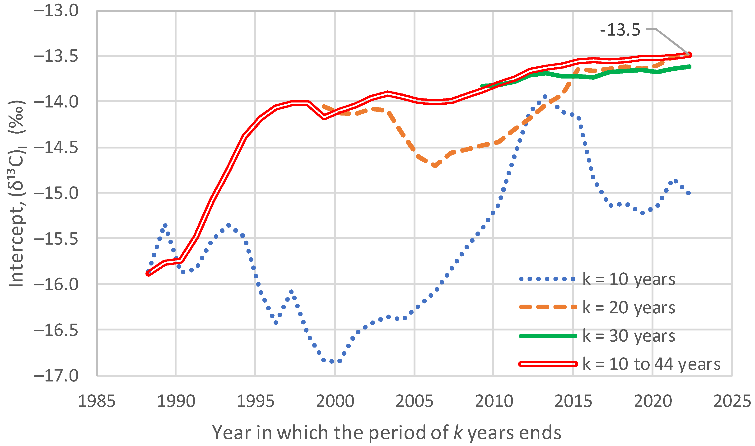
Specifically, we employ Equation (13) to find temporally averaged isotopic signatures over certain subperiods and investigate whether is decreasing with the progress of the time. Figure 11 shows an application of this idea to Mauna Loa, by considering subperiods (or windows) of a certain length k, which is fixed to 10, 20 or 30 years, sliding from the earlier to later times. This technique will be referred to as the fixed window length technique. No decreasing trend appears, while for the longer subperiod lengths, 20 and 30 years, the tendencies are clearly increasing, opposite to the hypothesis that they are caused by fossil fuel emissions.
In an alternative technique, referred to as the varying window length technique and also depicted in Figure 11, a window of varying length is considered with the start of the window fixed to the beginning of the observations and the end point moving forward from an offset of 10 years from the beginning to the end of the observations, so as to cover the entire period of observations (44 years). Now, the curve formed is persistently increasing, again contradicting the fossil fuel hypothesis.
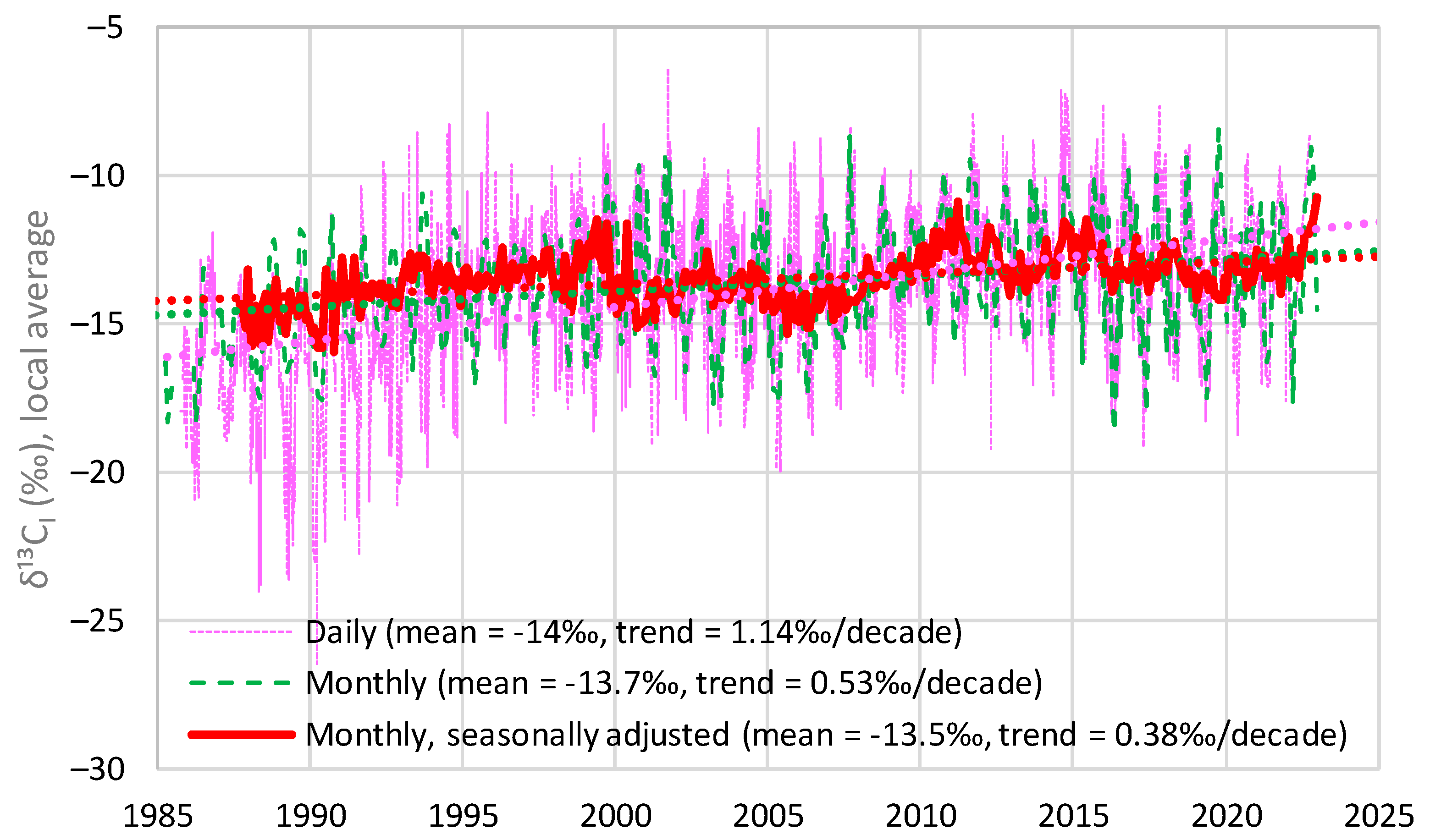
A third technique, referred to as the fixed difference technique is depicted in Figure 12, in which the window does not have a constant length but, for each ending point, the length is determined so that the difference in the denominator of Equation (13) is equal to the standard deviation of the observations. Note that for the earliest observations this is infeasible, and, for this reason, the horizontal (time) axis starts at a later time (1985). All three time series, daily, monthly and seasonally adjusted, are used. On the series of values determined, a trend line is fitted by linear regression and is plotted in the figure. In all cases, the trends are small (from 0.38‰/decade to 1.14‰/decade) and always positive, again contradicting the fossil fuel origin of the phenomenon.
Figure 13 shows the results of the fixed difference technique for all four sites examined. The trends vary from 0.27‰/decade for the South Pole to +0.38‰/decade for Mauna Loa. These values are small and not statistically significant even at the 5% level, as found by applying a Monte Carlo simulation technique, assuming a Hurst–Kolmogorov model for the simulation (see [29] and references therein) with the Hurst coefficient determined from the series of local averages. Therefore, for the modelling phase of Section 5 we will assume a constant over-year input isotopic signature , which, however, varies seasonally.
4.4. Proxy Data
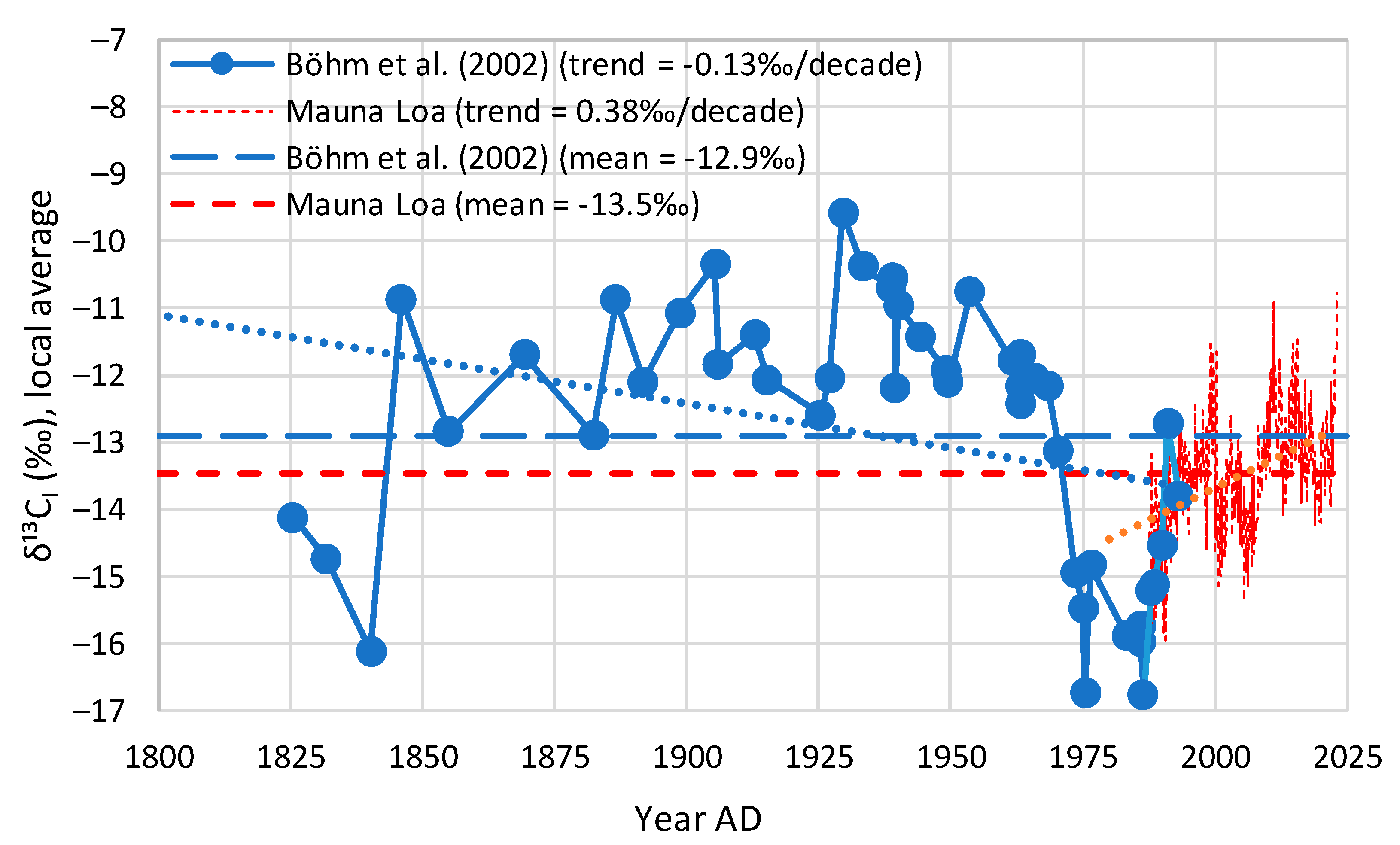
The Keeling plot of the proxy data, with a time period spanning from 1520 to 1997 AD, is depicted in Figure 14. The arrangement of points is fairly linear, resulting in an intercept of , which is, interestingly, the same as that seen in modern data. To investigate whether there is a temporal change in , we have split the sample into three subperiods, based on the quantity of human CO2 emissions, as seen in Table 2. The intercepts of the subperiods are shown in Figure 14. From the earliest period A to the next period B, there is a decrease in , which can hardly be attributed to human emissions, as these were not as large. From period B to C, we note an increase in , contradicting the fossil fuel attribution.
The fixed difference technique was also applied to the proxy data and the results are shown in Figure 15. Here we observe an alternation in increasing trends (early period before 1850 and latest period after 1975), stability (1850–1950) and a decreasing trend (1950–1975). The overall trend is decreasing but the latest period, 1975–1997, in which the human emissions were largest, is characterised by an increasing trend. Notably, the data values and the trend in the latest period agree with those of the instrumental Mauna Loa data, also plotted in Figure 15. Hence an attribution of the observed behaviour to human emissions again fails.
5. Modelling Results
5.1. Model Premises and Structure
After the diagnostic results of Section 5, we make the hypothesis that changes seen in the isotopic composition of the atmospheric are dominated by biosphere processes and neglect any effect of human emissions. Further, we consider that the Pinatubo eruption may have had an effect on the isotopic composition. As per ENSO, while we recognize that it affects the isotopic composition, we deem it unnecessary to explicitly model this effect, as its fingerprint may have already been present in , which is assumed to be a known input in our model. The purpose of this modelling exercise is to test if these hypotheses are consistent with the instrumental and proxy data.
The model we use is none other than the simple Equation (12), applied sequentially, each time using past and present data for , calculating the present value of from Equation (12). We run the model on a monthly time step (without any seasonal adjustment) for the sites with instrumental data, and, following the discussion in Section 3 and Section 4, we assume that the model has two parameters, , i.e., the input isotopic signatures for the seasonal increasing and decreasing phases of , respectively. Following the discussion in Section 3 (cf. Figure 5), we expect that will be lower than , for consistency with the over-year average. Following the results in Section 4, we expect the latter to be close to –13.2‰, even though we do not use this value in the modelling but rather we calculate it as a model result. In addition to the two parameters, we use two initial conditions, the first being the at the beginning of the simulation. As we recognize the role of the Pinatubo eruption, we assume that the regular course of the process was interrupted after the eruption, and we reinitialize the model a year after it with a second value . We determine the two parameters and the two initial conditions, , by minimizing the mean square error of the model fitting to the data.
In initial model runs we tested several cases and optimised the error at each site independently, trying different options of assigning the to each month. It was found that is fairly constant in all sites, while increases as we move from north to south. It was also found that the error is minimised if the input signature is assigned to the two months with the highest decrease in . These are July and August for the northern hemisphere, and November and December for the southern hemisphere ([2], Figure 7, right).
Based on these initial observations, we assumed that the value of is the same worldwide, while the value of is specific to the site. We thus found the single and the site-specific , by minimizing the sum of the fitting errors at all sites simultaneously.
In addition to the basic model run, in which the value of Equation (12) is taken to be the simulated value of the previous step, we perform another run, in which this value is updated at each step by the observation of the previous time step. The model parameters are kept the same as those used in the original model (without an update).
5.2. Model Application to Instrumental Data
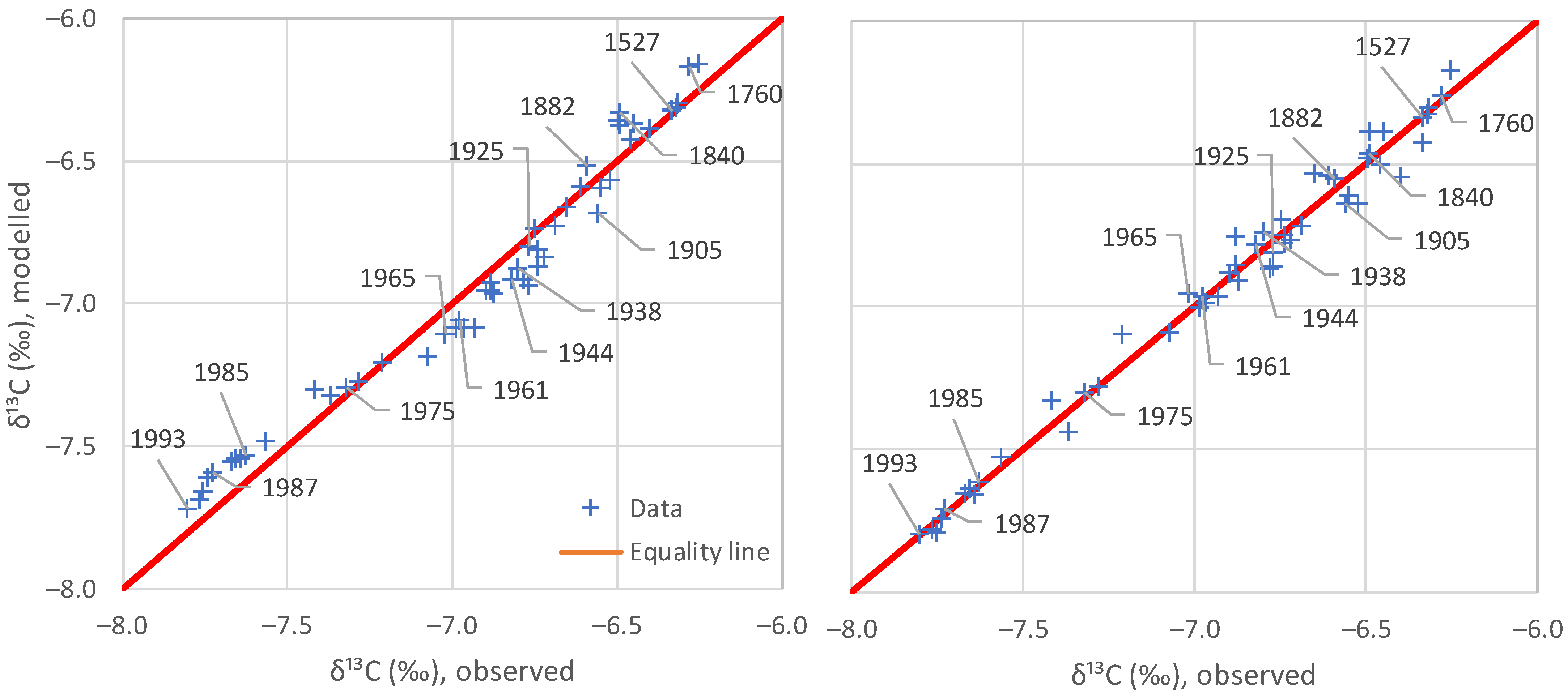
The model application is very easy due to the simplicity of the model and typical spreadsheet software with a solver to perform the error minimisation suffices. The values resulting from the error minimisation are shown in Table 3, along with the fitting metrics, namely the bias, which is zero in all cases, and the explained variance, which as high as 98–99%. (It should be noted that the explained variance is the remainder from 1 of the ratio of the variance of the model error to the variance of the modelled variable, and is otherwise known as the Nash–Sutcliffe efficiency.) In plain words, everything is very well reproduced by the model. The resulting fitting metrics in the model run with updated are also shown in Table 3 and are slightly better than those seen in the original model run.
5.3. Model Application to Proxy Data
The application of the model to proxy data is much simpler because the time scale is over-annual, without seasonality. Thus, a single value of suffices. This value is not optimised but taken as the average of the values over all four sites with instrumental data. With this choice, we test whether or not the modern values are also representative of the distant past, back to 1500 AD. The metrics of the model performance are also shown in Table 3 and are good, albeit not as good as the metrics seen in the instrumental data, which is justifiable for such a long period of time and for the large uncertainty discussed in Section 2.
6. Discussion
With only two parameters, , which represent the input isotopic signatures for the seasonal increasing and decreasing phases of , respectively, we are able to effectively model the isotopic signature of the atmosphere for the entire observation period. Of these parameters, , reflecting the fractionation by photosynthesis, can be assumed as the same for the entire globe, while varies, with smaller (more negative) values as we go north and higher (less negative) values as we go south. This spatial variation of reflects the differences of the strength of seasonality in and , which is at a maximum toward the North Pole and at a minimum at the South Pole. The strong seasonality at high latitudes north is probably related to the processes in boreal vegetation, the dominance of snow and ice in winter, and the absence of photosynthesis during the 6-month night (note that Barrow, at a latitude of 71.3° N, is more north that the Artic Circle at 66.6° N). As we go south, some of these features cease to occur, and seasonality becomes less prominent, as photosynthesis occurs throughout the entire year, albeit with varying intensities. The minimal seasonality in the South Pole is probably related to the absence of vegetation due to the minimal appearance of land beyond a latitude of 43° S (with the exception of the frozen continent of Antarctica and a relatively small wedge of land in South America). All these suggest the dominance of terrestrial biosphere processes in driving and .
Despite differences in seasonality, the over-annual input isotopic signature remains almost the same globally, as seen in Table 4, which summarizes the results of all analyses, diagnostic and modelling, suggesting similar values, irrespective of the method used. This is not difficult to explain as, in the long run, is well mixed in the atmosphere; thus regional differences in seasonal tend to disappear.
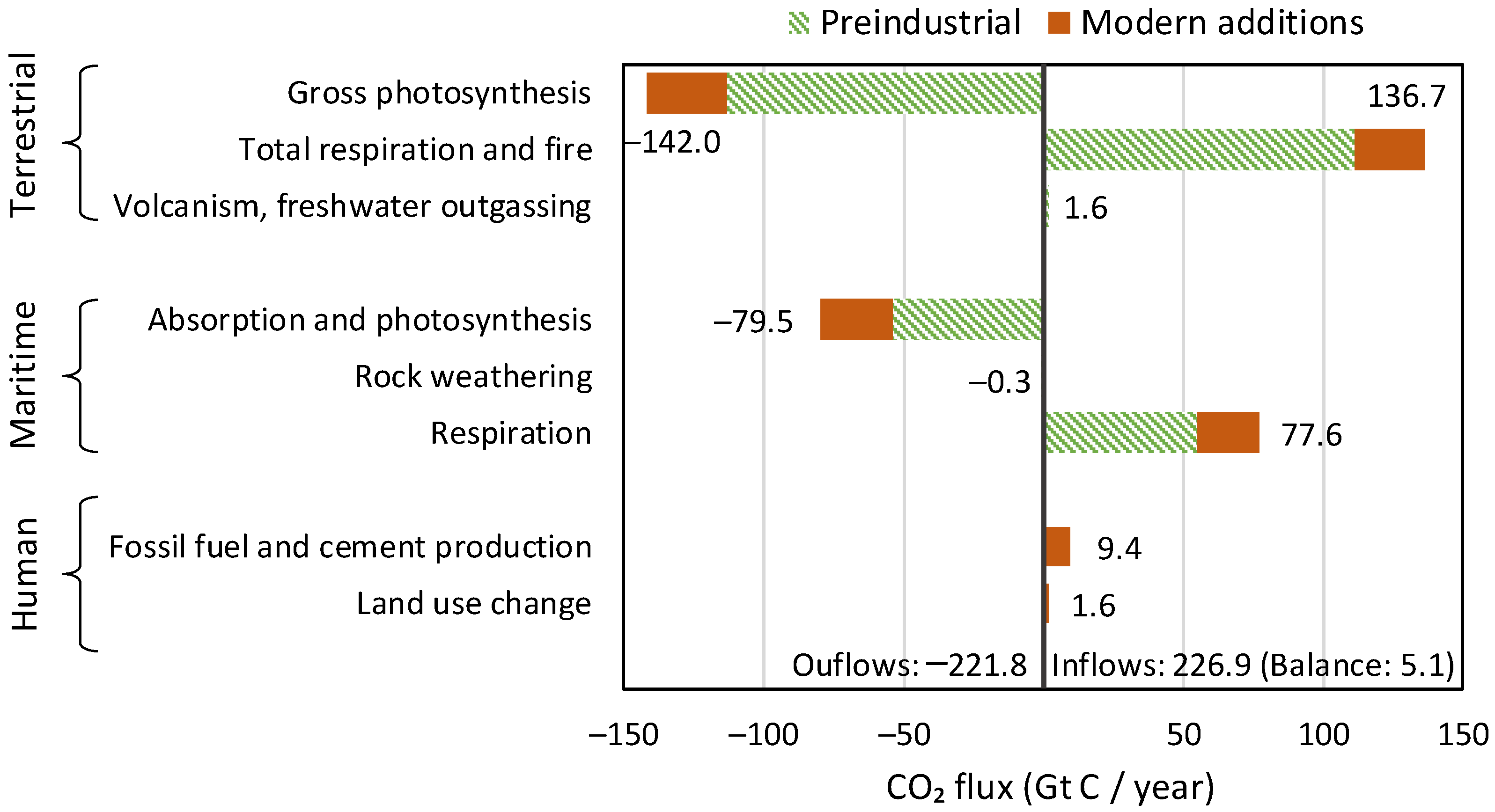
In both the diagnostic and the modelling phases of this paper, the inclusion of human emissions proved unnecessary. This may contrast with common opinion, which blames all changes on humans, but is absolutely reasonable, as humans are responsible for only 4% of carbon emissions. In addition, the vast majority of changes in the atmosphere since 1750 are due to natural processes, respiration and photosynthesis, as articulated in the recent study by Koutsoyiannis et al. [5] and schematically depicted in Figure 22, reproduced from that study.
The following observations can be noted in Figure 22: (a) the terrestrial biosphere processes are much stronger than the maritime ones in terms of both production and absorption of CO2; (b) the CO2 emissions by even the ocean biosphere are much larger than human emissions; and (c) the modern (post 1750) CO2 additions to pre-industrial quantities (red bars in the right-hand part of the graph, corresponding to positive values) exceed the human emissions by a factor of ~4.5. These observations provide explanations for the findings of this study.
Furthermore, it is relevant to note the minor role of CO2 in the greenhouse effect. As shown in a recent study by Koutsoyiannis and Vournas [31], despite the increase in [CO2] by more than 30% in a century-long period, the strength of the greenhouse effect has not changed in a manner discernible in the radiation data. The greenhouse effect is dominated by the presence of water vapour in the atmosphere, rather than CO2.
7. Conclusions
The results of the analyses in this paper provide negative answers to the research questions posed in the Introduction. Specifically:
- From modern instrumental carbon isotopic data of the last 40 years, no signs of human (fossil fuel) CO2 emissions can be discerned;
- Proxy data since the Little Ice Age suggest that the modern period of instrumental data does not differ, in terms of the net isotopic signature of atmospheric CO2 sources and sinks, from earlier centuries.
Combined with earlier studies, namely [2,3,4,5,31], these findings allow for the following line of thought to be formulated, which contrasts the dominant climate narrative, on the basis that different lines of thought are beneficial for the progress of science, even though they are not welcomed by those with political agendas promoting the narratives (whose representatives declare that they “own the science”, as can be seen in the motto in the beginning of the paper).
- It the 16th century, Earth entered a cool climatic period, known as the Little Ice Age, which ended at the beginning of the 19th century;
- Immediately after, a warming period began, which has lasted until now. The causes of the warming must be analogous to those that resulted in the Medieval Warm Period around 1000 AD, the Roman Climate Optimum around the first centuries BC and AD, the Minoan Climate Optimum at around 1500 BC, and other warming periods throughout the Holocene;
- As a result of the increased CO2 concentration, the isotopic signature δ13C in the atmosphere has decreased;
- The greenhouse effect on the Earth remained stable in the last century, as it is dominated by the water vapour in the atmosphere [31];
- Human CO2 emissions have played a minor role in the recent climatic evolution, which is hardly discernible in observational data and unnecessary to invoke in modelling the observed behaviours, including the change in the isotopic signature δ13C in the atmosphere.
Overall, the findings in this paper confirm the major role of the biosphere in the carbon cycle (and through this in climate) and a non-discernible signature of humans.
One may associate the findings of the paper with several questions related to international policies. Do these results refute the hypothesis that CO2 emissions contribute to global warming through the greenhouse effect? Do these findings, by suggesting a minimal human impact on the isotopic composition of atmospheric carbon, contradict the need to reduce CO2 emissions? Are human carbon emissions independent from other forms of pollution, such as emissions of fine particles and nitrogen oxides, which can have harmful effects on human health and the environment? These questions are not posed at all in the paper and certainly are not studied in it. Therefore, they cannot be answered on a scientific basis within the paper’s confined scope but require further research. The reader may feel free to study such questions and provide sensible replies. It is relevant to note that a reviewer implied these questions and suggested negative replies to each of them.
Funding
This research received no funding but was conducted for scientific curiosity.
Institutional Review Board Statement
Not applicable.
Informed Consent Statement
Not applicable.
Data Availability Statement
This research uses no new data. The data sets used have been retrieved from the sources described in detail in the text.
Acknowledgments
I am grateful to Jim Ross (independent researcher, Scotland) who shared with me his observations regarding the δ13C of atmospheric CO2 growth. I thank him for his critical comments on earlier drafts and analyses and I regret that we were not able to produce a joint paper. I am also thankful to three reviewers for their constructive comments, which helped me to improve the paper.
Conflicts of Interest
The author declares no conflicts of interest.
Appendix A. Calculations of a Two-Step Cycle of CO2 Seasonal Change
In Section 3, we assumed a system with periodic increases and decreases in within a year. As discussed in Section 3, only the initial and final conditions in the studied period matter and not the path between them. Hence, for simplicity, we assume that the beginning of the period coincides with the beginning of the rising . We assume initial conditions (). Further, we assume that in the first step, the system receives an input with the constant isotopic ratio and increases its concentration to , and in a second step, the concentration is decreased to by absorption by a net sink with fractionation, so that the isotopic ratio is (the subscripts U and D denote up and down, respectively). The first step is described by:
and the second step is described by
Eliminating , we find:
or
which yields:
On the other hand, if and if we express in terms of the average of the entire cycle (both steps), we have:
Equating the right-hand sides of Equations (A5) and (A6) we obtain
and solving for , we find:
By dividing by and using the definitions of Equation (15) we conclude with Equation (14).
References
- Bernstein, B.M. U.N. Communications Official Touts Google Search Partnership: ‘We Own the Science’, National Review, 4 October 2022. Available online: https://www.nationalreview.com/news/u-n-communications-official-touts-google-search-partnership-we-own-the-science/ (accessed on 15 December 2023).
- Koutsoyiannis, D.; Kundzewicz, Z.W. Atmospheric temperature and CO2: Hen-or-egg causality? Sci 2020, 2, 83. [Google Scholar] [CrossRef]
- Koutsoyiannis, D.; Onof, C.; Christofides, A.; Kundzewicz, Z.W. Revisiting causality using stochastics: 1. Theory. Proc. R. Soc. A 2022, 478, 20210836. [Google Scholar] [CrossRef]
- Koutsoyiannis, D.; Onof, C.; Christofides, A.; Kundzewicz, Z.W. Revisiting causality using stochastics: 2. Applications. Proc. R. Soc. A 2022, 478, 20210835. [Google Scholar] [CrossRef]
- Koutsoyiannis, D.; Onof, C.; Kundzewicz, Z.W.; Christofides, A. On Hens, Eggs, Temperatures and CO2: Causal Links in Earth’s Atmosphere. Sci 2023, 5, 35. [Google Scholar] [CrossRef]
- Climate Etc. (Judith Curry’s Blog), Causality and Climate. 2023. Available online: https://judithcurry.com/2023/09/26/causality-and-climate/ (accessed on 15 November 2023).
- Christofides, A.; Koutsoyiannis, D.; Onof, C.; Kundzewicz, Z.W. Causality, Climate, Etc. ResearchGate 2023. [Google Scholar] [CrossRef]
- Graven, H.; Keeling, R.F.; Rogelj, J. Changes to carbon isotopes in atmospheric CO2 over the industrial era and into the future. Glob. Biogeochem. Cycles 2020, 34, e2019GB006170. [Google Scholar] [CrossRef] [PubMed]
- Craig, H. Isotopic standards for carbon and oxygen and correction factors for mass spectrometric analysis of carbon dioxide, Geochim. Cosmochim. Acta 1957, 12, 133–149. [Google Scholar] [CrossRef]
- Lueker, T.; Keeling, R.; Bollenbacher, A.; Walker, S.; Morgan, E.; Brooks, M. Calibration Methodology for the Scripps 13C/12C and 18O/16O Stable Isotope Program. 2020. Available online: https://escholarship.org/uc/item/4n93p288 (accessed on 15 November 2023).
- Suess, H.E. Radiocarbon concentration in modern wood. Science 1955, 122, 415–417. [Google Scholar] [CrossRef]
- Graven, H.; Allison, C.E.; Etheridge, D.M.; Hammer, S.; Keeling, R.F.; Levin, I.; Meijer, H.A.; Rubino, M.; Tans, P.P.; Trudinger, C.M.; et al. Compiled records of carbon isotopes in atmospheric CO2 for historical simulations in CMIP6. Geosci. Model Dev. 2017, 10, 4405–4417. [Google Scholar] [CrossRef]
- Ritchie, H.; Roser, M. CO2 Emissions. OurWorldInData.org. 2020. Available online: https://ourworldindata.org/co2-emissions (accessed on 15 December 2023).
- Global Carbon Budget (2023)—With Major Processing by Our World in Data. “Annual CO2 Emissions—GCB” [Dataset]. Global Carbon Project, “Global Carbon Budget” [Original Data]. Available online: https://ourworldindata.org/co2-and-greenhouse-gas-emissions (accessed on 15 December 2023).
- Andres, R.J.; Marland, G.; Boden, T.; Bischof, S. Carbon Dioxide Emissions from Fossil Fuel Consumption and Cement Manufacture, 1751-1991; And an Estimate of Their Isotopic Composition and Latitudinal Distribution (No. CONF-9307181-4); Oak Ridge National Laboratory: Oak Ridge, TN, USA; Oak Ridge Institute for Science and Education: Oak Ridge, TN, USA, 1994. Available online: https://www.osti.gov/servlets/purl/10185357 (accessed on 15 December 2023).
- Andres, R.J.; Marland, G.; Boden, T.; Bischof, S. Carbon dioxide emissions from fossil fuel consumption and cement manufacture, 1751–1991, and an estimate of their isotopic composition and latitudinal distribution. In The Carbon Cycle; Wigley, T.M., Schimel, D.S., Eds.; Cambridge University Press: Cambridge, UK, 2000; pp. 53–62. [Google Scholar]
- Zhu, Z.; Piao, S.; Myneni, R.B.; Huang, M.; Zeng, Z.; Canadell, J.G.; Ciais, P.; Sitch, S.; Friedlingstein, P.; Arneth, A.; et al. Greening of the Earth and its drivers. Nat. Clim. Change 2016, 6, 791–795. [Google Scholar] [CrossRef]
- Chen, C.; Park, T.; Wang, X.; Piao, S.; Xu, B.; Chaturvedi, R.K.; Fuchs, R.; Brovkin, V.; Ciais, P.; Fensholt, R.; et al. China and India lead in greening of the world through land-use management. Nat. Sustain. 2019, 2, 122–129. [Google Scholar] [CrossRef] [PubMed]
- Li, Y.; Li, Z.L.; Wu, H.; Zhou, C.; Liu, X.; Leng, P.; Yang, P.; Wu, W.; Tang, R.; Shang, G.F.; et al. Biophysical impacts of earth greening can substantially mitigate regional land surface temperature warming. Nat. Commun. 2023, 14, 121. [Google Scholar] [CrossRef] [PubMed]
- Keeling, C.D.; Piper, S.C.; Whorf, T.P.; Keeling, R.F. Evolution of natural and anthropogenic fluxes of atmospheric CO2 from 1957 to 2003. Tellus B Chem. Phys. Meteorol. 2011, 63, 1–22. [Google Scholar] [CrossRef]
- Scripps CO2 Program, Sampling Station Records. Available online: https://scrippsco2.ucsd.edu/data/atmospheric_co2/sampling_stations.html (accessed on 15 November 2023).
- Keeling, C.D.; Piper, S.C.; Bacastow, R.B.; Wahlen, M.; Whorf, T.P.; Heimann, M.; Meijer, H.A. Exchanges of Atmospheric CO2 and 13CO2 with the Terrestrial Biosphere and Oceans from 1978 to 2000. I. Global Aspects; SIO Reference Series No. 01-06; Scripps Institution of Oceanography: San Diego, CA, USA, 2001; 28p. [Google Scholar]
- Keeling, C.D.; Piper, S.C.; Bacastow, R.B.; Wahlen, M.; Whorf, T.P.; Heimann, M.; Meijer, H.A. Atmospheric CO2 and 13CO2 exchange with the terrestrial biosphere and oceans from 1978 to 2000: Observations and carbon cycle implications. In A History of Atmospheric CO2 and Its Effects on Plants; Ehleringer, J.R., Cerling, T.E., Dearing, M.D., Eds.; Springer: New York, NY, USA, 2005; pp. 83–113. [Google Scholar]
- Böhm, F.; Haase-Schramm, A.; Eisenhauer, A.; Dullo, W.C.; Joachimski, M.M.; Lehnert, H.; Reitner, J. Evidence for preindustrial variations in the marine surface water carbonate system from coralline sponges. Geochem. Geophys. Geosyst. 2002, 3, 1–13. [Google Scholar] [CrossRef]
- Keeling, C.D. The concentration and isotopic abundance of carbon dioxide in rural areas. Geochim. Cosmochim. Acta 1958, 13, 322–334. [Google Scholar] [CrossRef]
- Keeling, C.D. The concentration and isotopic abundance of carbon dioxide in rural and marine air. Geochim. Cosmochim. Acta 1961, 24, 277–298. [Google Scholar] [CrossRef]
- Miller, J.B.; Tans, P.P. Calculating isotopic fractionation from atmospheric measurements at various scales. Tellus B Chem. Phys. Meteorol. 2003, 55, 207–214. [Google Scholar] [CrossRef]
- Köhler, P.; Fischer, H.; Schmitt, J.; Munhoven, G. On the application and interpretation of Keeling plots in paleo climate research–deciphering δ13C of atmospheric CO2 measured in ice cores. Biogeosciences 2006, 3, 539–556. [Google Scholar] [CrossRef]
- Koutsoyiannis, D. Stochastics of Hydroclimatic Extremes–A Cool Look at Risk, 3rd ed.; Kallipos Open Academic Editions: Athens, Greece, 2023; 391p, ISBN 978-618-85370-0-2. [Google Scholar] [CrossRef]
- IPCC. Climate Change 2021: The Physical Science Basis. In Contribution of Working Group I to the Sixth Assessment Report of the Intergovernmental Panel on Climate Change; Masson-Delmotte, V.P., Zhai, A., Pirani, S.L., Connors, C., Péan, S., Berger, N., Caud, Y., Chen, L., Goldfarb, M.I., Gomis, M., et al., Eds.; Cambridge University Press: Cambridge, UK; New York, NY, USA, 2021; 2391p. [Google Scholar] [CrossRef]
- Koutsoyiannis, D.; Vournas, C. Revisiting the greenhouse effect—A hydrological perspective. Hydrol. Sci. J. 2024, 69, 151–164. [Google Scholar] [CrossRef]
- Chen, X.; Chen, T.; He, B.; Liu, S.; Zhou, S.; Shi, T. The global greening continues despite increased drought stress since 2000. Glob. Ecol. Conserv. 2024, 49, e02791. [Google Scholar] [CrossRef]
Figure 1.
Typical ranges of isotopic signatures δ13C for each of the pools interacting with atmospheric CO2, and related exchange processes. Processes involving significant fractionation (gas exchange, photosynthesis) or not are shown in italics or upright fonts, respectively. The highest and lowest values appearing, 2‰ and −44‰, respectively, correspond to ratios 11.237453‰ and 11.231644‰, respectively, while the PDB standard ratio is 11.2372‰ (reproduced from Graven et al. [8], licensed under Creative Commons Attribution).

Figure 2.
(left) Compiled data set of annual mean, global mean values for δ13C in atmospheric CO2, from Graven et al. [12], reconstructed after digitisation of Figure 3 of Graven et al. [8]; and (right) evolution of global human carbon emissions [13,14], after conversion from CO2 to C (dividing by 3.67).

Figure 3.
(left) Reproduction of Figure 4 of Böhm et al. [24] after digitisation (for the indicated variables for the atmosphere only); and (right) comparison of the curves of Böhm et al. [24] (from the left panel) and Graven et al. [8] (from Figure 2).

Figure 4.
(left) Keeling plots (δ13C vs. 1/[CO2]) assuming initial conditions and [CO2]0 = 280 ppm, and various input isotopic signatures which are multiples of −6‰; (right) time series plot of δ13C, obtained by transformation of the left graph into one of temporal evolution of δ13C, assuming that the temporal evolution of [CO2] resembles the actual one in the Earth’s atmosphere after 1500 AD, approximated as [CO2]/ppm = exp(0.0174 (year − 1500) − 4.3154) + 280, which was a fitted on the [CO2] curve of Figure 3.

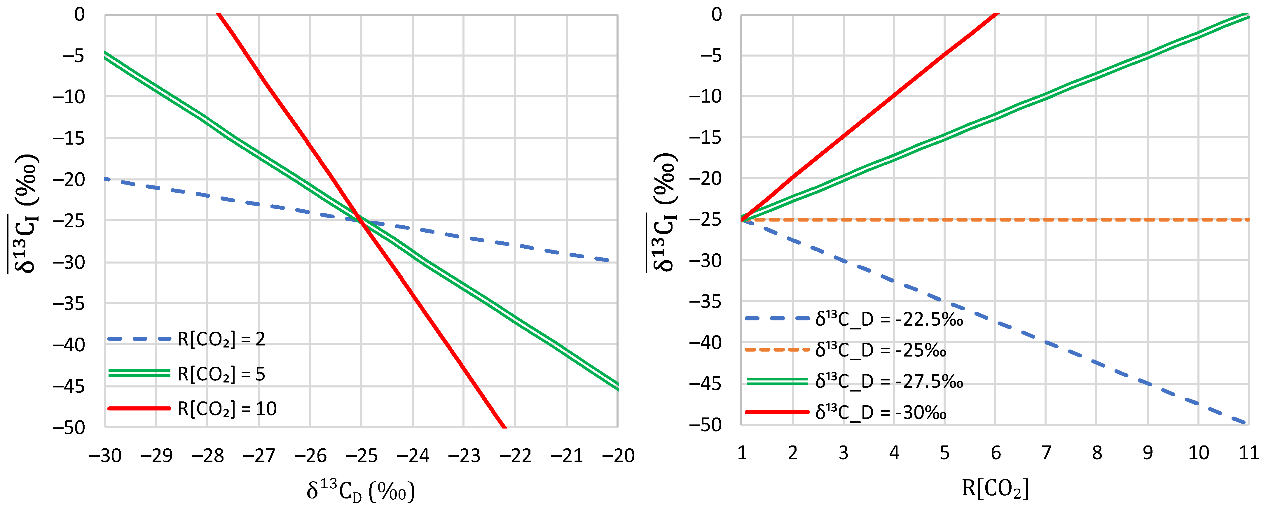
Figure 5.
Variation of the over-year average as a function of (left) the seasonal during the absorption phase and (right) the ratio of seasonal increase to annual increase, . In both graphs the seasonal during the growth phase is −25‰, close to the value estimated from the data for the northern hemisphere. The double green lines are consistent with the estimates from the data (see Section 4).

Figure 6.
(upper) Comparative plot of the monthly instrumental time series of in at the investigated four sites; (lower) annual range (maximum minus minimum value per year) for each of the four time series.
Figure 6.
(upper) Comparative plot of the monthly instrumental time series of in at the investigated four sites; (lower) annual range (maximum minus minimum value per year) for each of the four time series.

Figure 7.
Focus on a decade of the in atmospheric , compared to the corresponding , for the monthly time series at Mauna Loa.
Figure 7.
Focus on a decade of the in atmospheric , compared to the corresponding , for the monthly time series at Mauna Loa.

Figure 8.
Keeling plots of the Mauna Loa time series, where the abscissa 1/[CO2] and the ordinate are simultaneous observations (daily or monthly measurements and seasonally adjusted values as provided by the Scripps CO2 Program) and the points that are consecutive in time are connected with straight lines.

Figure 9.
Keeling plots of the (upper) Barrow and (lower) South Pole time series, where the abscissa 1/[CO2] and the ordinate are simultaneous observations (daily or monthly measurements and seasonally adjusted values as provided by the Scripps CO2 Program) and the points that are consecutive in time are connected with straight lines.

Figure 10.
Keeling plots of the indicated time series adjusted for seasonality.

Figure 11.
Intercept calculated from daily Mauna Loa data for subperiods with the indicated length k, ending at the indicated year in the horizontal axis.
Figure 11.
Intercept calculated from daily Mauna Loa data for subperiods with the indicated length k, ending at the indicated year in the horizontal axis.

Figure 12.
Local average of input isotopic signatures calculated from the indicated Mauna Loa time series for periods with a varying length, ending at the indicated year in the horizontal axis, and a constant increase in [CO2], equal to the standard deviation of each of the time series.
Figure 12.
Local average of input isotopic signatures calculated from the indicated Mauna Loa time series for periods with a varying length, ending at the indicated year in the horizontal axis, and a constant increase in [CO2], equal to the standard deviation of each of the time series.

Figure 13.
Local average of input isotopic signatures calculated from the indicated time series adjusted for seasonality for periods with varying lengths, ending at the indicated year in the horizontal axis, using the fixed difference technique.
Figure 13.
Local average of input isotopic signatures calculated from the indicated time series adjusted for seasonality for periods with varying lengths, ending at the indicated year in the horizontal axis, using the fixed difference technique.


Figure 15.
Local average of input isotopic signatures calculated from the Böhm et al. [24] proxy data for periods with varying lengths, ending at the indicated year in the horizontal axis, using the fixed difference technique. For comparison, the local averages of the Mauna Loa seasonally adjusted time series are also plotted.

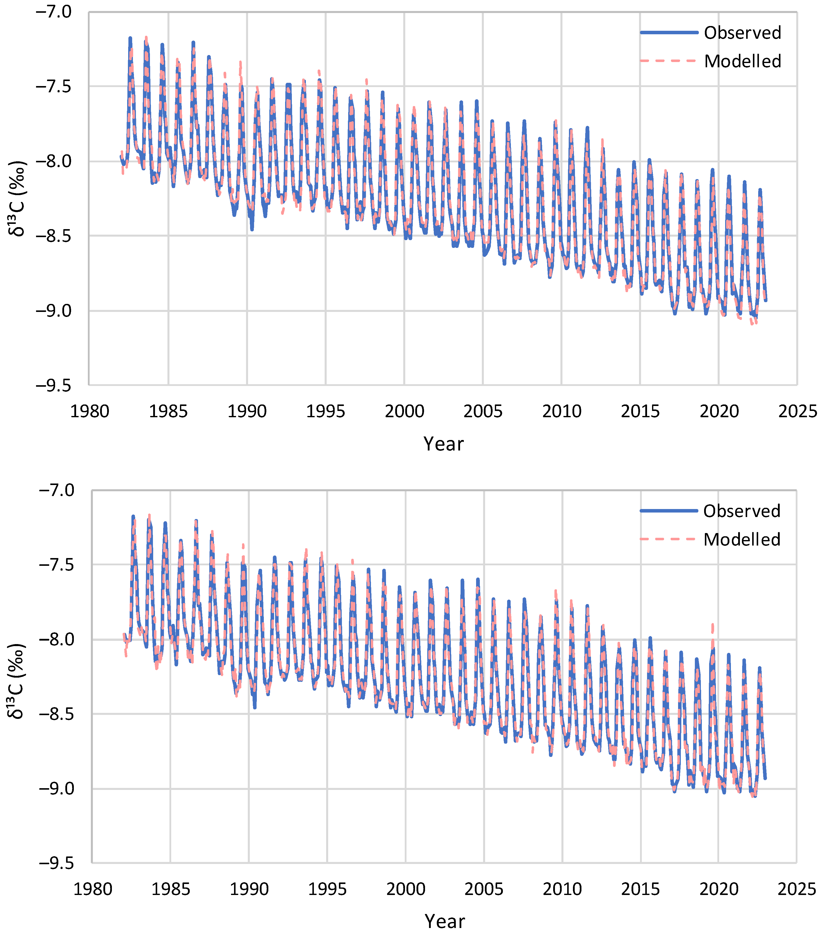
Figure 16.
Model reproduction of the monthly observations of evolution of at Barrow: (upper) without update of initial conditions and (lower) with update of initial conditions in each step by the observations.
Figure 16.
Model reproduction of the monthly observations of evolution of at Barrow: (upper) without update of initial conditions and (lower) with update of initial conditions in each step by the observations.

Figure 17.
Model reproduction of the monthly observations of evolution of at the South Pole: (upper) without update of initial conditions and (lower) with update of initial conditions in each step by the observations.
Figure 17.
Model reproduction of the monthly observations of evolution of at the South Pole: (upper) without update of initial conditions and (lower) with update of initial conditions in each step by the observations.

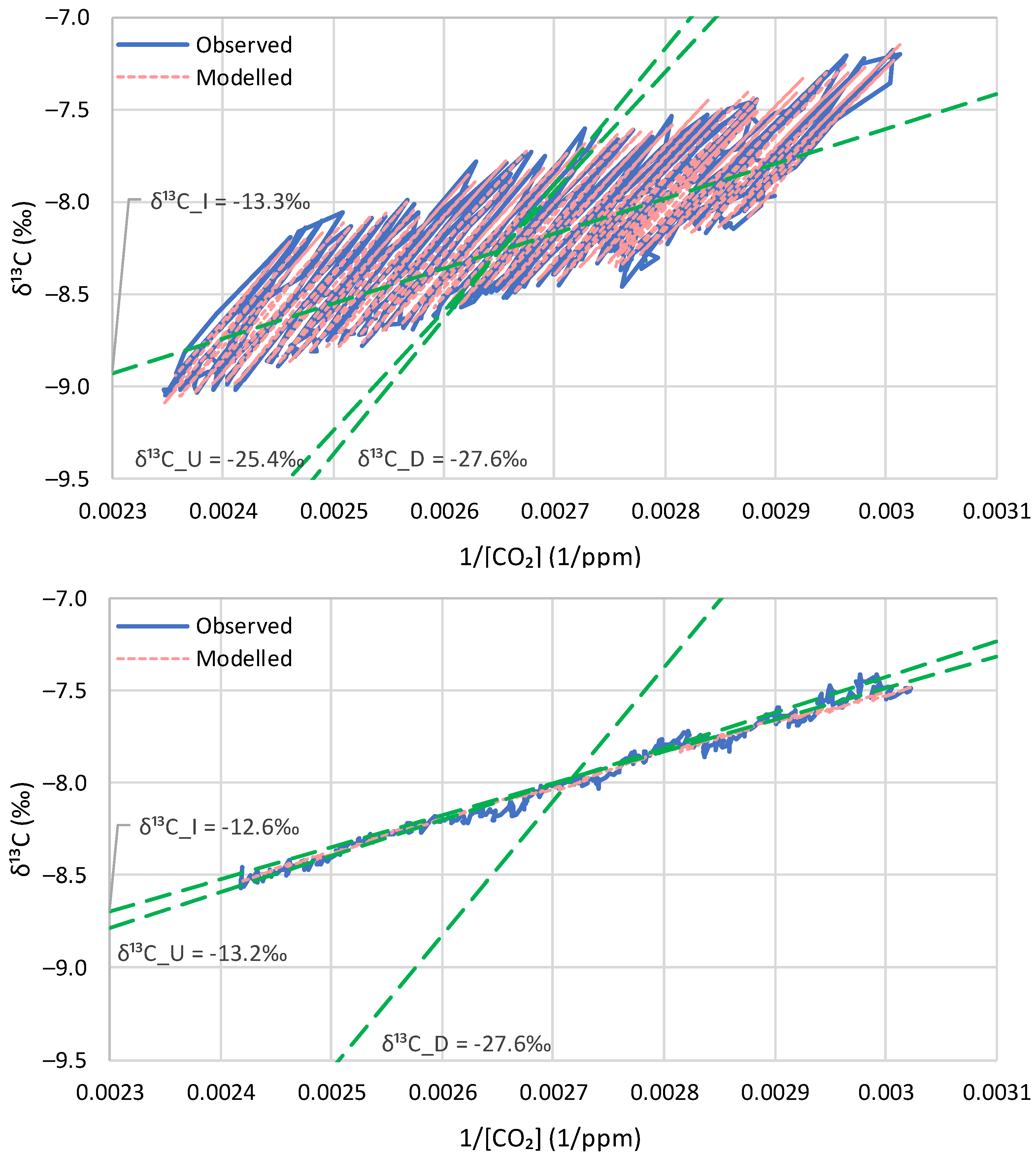
Figure 18.
Keeling plot of the monthly observations of at (upper) Barrow and (lower) the South Pole for the original model mode, without updates. The constant input isotopic signatures of and for the seasonal increasing and decreasing phases of (model parameters), as well as the over-year (model result), are also depicted by means of straight lines passing from the centre of gravity with the indicated intercepts marked.

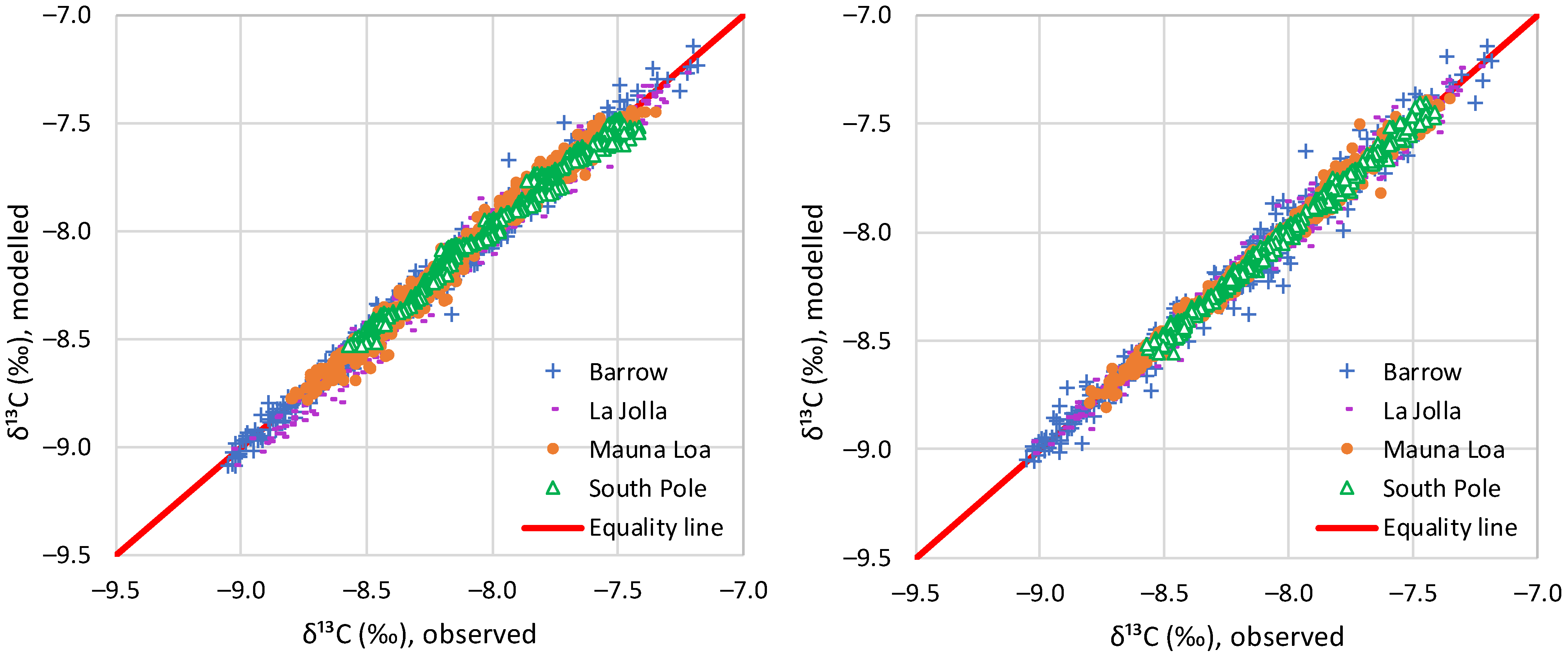
Figure 19.
Model reproduction of the monthly observations of at the four sites: (left) without update of initial conditions and (right) with update of initial conditions in each step by the observations.
Figure 19.
Model reproduction of the monthly observations of at the four sites: (left) without update of initial conditions and (right) with update of initial conditions in each step by the observations.

Figure 20.
Model reproduction of Böhm et al. [24] proxy series of as (left column) a time series plot and (right column) a Keeling plot; (upper row) without update of initial conditions and (lower row) with update of initial conditions in each step by the observations. For better graphical interpretation of the right panels, the straight line passing from the centre of gravity with intercept is also shown (green dashed line).

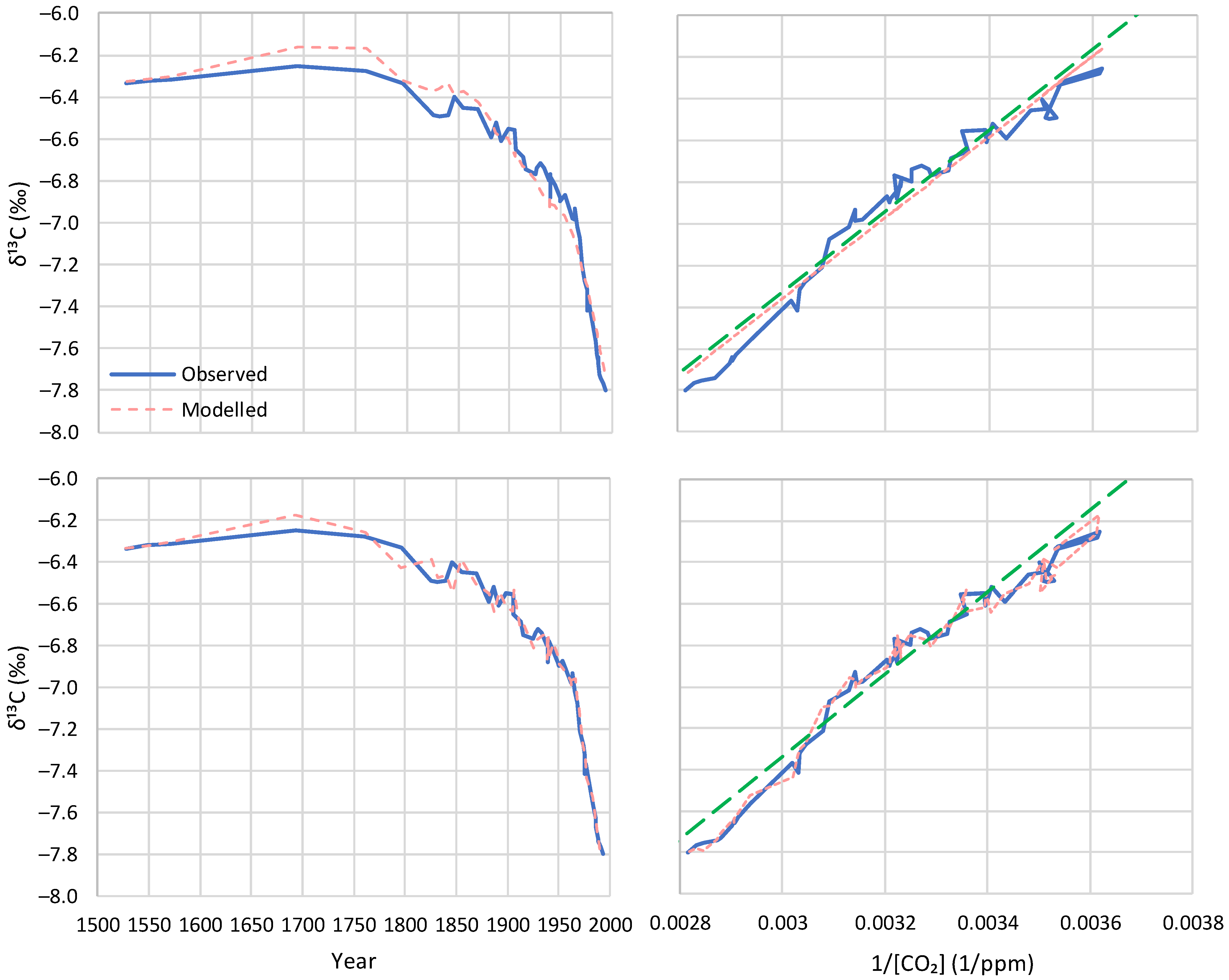
Figure 21.
Model reproduction of Böhm et al. [24] proxy series of , (left) without update of initial conditions and (right) with update of initial conditions in each step by the observation. A constant input isotopic signature is used.
Figure 21.
Model reproduction of Böhm et al. [24] proxy series of , (left) without update of initial conditions and (right) with update of initial conditions in each step by the observation. A constant input isotopic signature is used.

Figure 22.
Annual carbon balance in the Earth’s atmosphere, in Gt C/year, based on the IPCC estimates (Figure 5.12 of [30]). The balance of 5.1 Gt C/year is the annual accumulation of carbon (in the form of CO2) in the atmosphere (reproduced from [5].).


Table 1.
Observation sites with isotopic data on atmospheric CO2 and their characteristics.
| Station Name | Station Code | Latitude | Longitude | Elevation (m) | Dates |
|---|---|---|---|---|---|
| Barrow, Alaska | PTB | 71.3° N | 156.6° W | 11 | 1982–present |
| La Jolla Pier, California | LJO | 32.9° N | 117.3° W | 10 | 1978–present |
| Mauna Loa Observatory, Hawaii | MLO | 19.5° N | 155.6° W | 3397 | 1978–present |
| South Pole | SPO | 90.0° S | 2810 | 1977–present |
Table 2.
Designation of subperiods in Böhm et al. [24] proxy data.
Table 2.
Designation of subperiods in Böhm et al. [24] proxy data.
| Subperiod | Years | Human CO2 Emissions, Gt C/Year | [CO2], ppm | # Data Points of |
|---|---|---|---|---|
| A | 1520–1898 | 0–0.5 | 283–295 | 16 |
| B | 1899–1976 | 0.5–5 | 296–330 | 27 |
| C | 1977–1997 | >5 | >331 | 10 |
Table 3.
Model parameters and performance indices for (‰).
| Time Series | ‰ | , ‰ (Months of Application) | Initial Conditions ‰) | ‰ w/o Update (w/Update) | Bias (%) w/o Update (w/Update) | Explained Variance (%) w/o Update (w/Update) |
|---|---|---|---|---|---|---|
| Barrow | −25.4 | −27.6 (6,7) | −7.9 (−8.4) | −13.3 (−13.3) | 0.0 (0.0) | 98.7 (98.2) |
| La Jolla | −24.6 | −27.6 (6,7) | −7.8 (−8.2) | −13.5 (−13.5) | 0.0 (0.0) | 97.8 (98.2) |
| Mauna Loa | −21.2 | −27.6 (6,7) | −7.6 (−8.0) | −13.3 (−13.3) | 0.0 (0.0) | 98.1 (98.9) |
| South Pole | −13.2 | −27.6 (11,12) | −7.5 (−7.8) | −12.6 (−12.6) | 0.0 (0.0) | 98.6 (99.5) |
| Proxy, Böhm et al. [24] | −13.2 | −13.2 (n/a) | −6.3 (n/a) | −13.2 (−13.2) | 0.0 (0.0) | 95.9 (98.4) |
Table 4.
Summary of results of input over-annual isotopic signatures (‰).
| Time Series | Keeling Plot Intercept | Mean (and Linear Trend) of Local Averages of | Long-Term Average from Model |
|---|---|---|---|
| Barrow | −13.2 | −13.3 (+0.07) | −13.3 |
| La Jolla | −13.3 | −13.5 (−0.08) | −13.5 |
| Mauna Loa | −13.3 | −13.5 (+0.38) | −13.3 |
| South Pole | −12.9 | −12.7 (−0.27) | −12.6 |
| Proxy, Böhm et al. [24] | −13.3 | −12.9 (−0.13) | −13.2 |
| Average | −13.2 | −13.2 (+0.01) | −13.2 |
Disclaimer/Publisher’s Note: The statements, opinions and data contained in all publications are solely those of the individual author(s) and contributor(s) and not of MDPI and/or the editor(s). MDPI and/or the editor(s) disclaim responsibility for any injury to people or property resulting from any ideas, methods, instructions or products referred to in the content. |
© 2024 by the author. Licensee MDPI, Basel, Switzerland. This article is an open access article distributed under the terms and conditions of the Creative Commons Attribution (CC BY) license (https://creativecommons.org/licenses/by/4.0/).
Share and Cite
MDPI and ACS Style
Koutsoyiannis, D. Net Isotopic Signature of Atmospheric CO2 Sources and Sinks: No Change since the Little Ice Age. Sci 2024, 6, 17. https://0-doi-org.brum.beds.ac.uk/10.3390/sci6010017
AMA Style
Koutsoyiannis D. Net Isotopic Signature of Atmospheric CO2 Sources and Sinks: No Change since the Little Ice Age. Sci. 2024; 6(1):17. https://0-doi-org.brum.beds.ac.uk/10.3390/sci6010017
Chicago/Turabian StyleKoutsoyiannis, Demetris. 2024. "Net Isotopic Signature of Atmospheric CO2 Sources and Sinks: No Change since the Little Ice Age" Sci 6, no. 1: 17. https://0-doi-org.brum.beds.ac.uk/10.3390/sci6010017