Passenger Flow Prediction of Urban Rail Transit Based on Deep Learning Methods

1
Department of Engineering Physics, Tsinghua University, Beijing 100084, China
2
Beijing Research Center of Urban Systems Engineering, Beijing 100035, China
3
Institute of Science and Development, Chinese Academy of Sciences, Beijing 100190, China
*
Author to whom correspondence should be addressed.
Smart Cities 2019, 2(3), 371-387; https://0-doi-org.brum.beds.ac.uk/10.3390/smartcities2030023
Submission received: 28 May 2019
/
Revised: 12 June 2019
/
Accepted: 16 July 2019
/
Published: 23 July 2019
(This article belongs to the Special Issue Big Data-Driven Intelligent Services in Smart Cities)
Abstract
:The rapid development of urban rail transit brings high efficiency and convenience. At the same time, the increasing passenger flow also remarkably increases the risk of emergencies such as passenger stampedes. The accurate and real-time prediction of dynamic passenger flow is of great significance to the daily operation safety management, emergency prevention, and dispatch of urban rail transit systems. Two deep learning neural networks, a long short-term memory neural network (LSTM NN) and a convolutional neural network (CNN), were used to predict an urban rail transit passenger flow time series and spatiotemporal series, respectively. The experiments were carried out through the passenger flow of Beijing metro stations and lines, and the prediction results of the deep learning methods were compared with several traditional linear models including autoregressive integrated moving average (ARIMA), seasonal autoregressive integrated moving average (SARIMA), and space–time autoregressive integrated moving average (STARIMA). It was shown that the LSTM NN and CNN could better capture the time or spatiotemporal features of the urban rail transit passenger flow and obtain accurate results for the long-term and short-term prediction of passenger flow. The deep learning methods also have strong data adaptability and robustness, and they are more ideal for predicting the passenger flow of stations during peaks and the passenger flow of lines during holidays.
1. Introduction
With the continuous formation and expansion of urban rail transit networks, this transportation mode brings high efficiency and convenience to residents’ travel. However, its increasing passenger flow also remarkably increases the risk of emergencies such as crowded passengers and stampedes. In the urban rail transit intelligent system, the accurate and real-time prediction of dynamically changing passenger flow is of great significance to the daily operation safety management, emergency prevention, and dispatch of urban rail transit. Many researchers have proposed some methods for the passenger flow prediction of urban rail transit, as well as road traffic prediction. These studies mainly used historical time series or spatiotemporal series with certain time intervals—combined with other auxiliary information—and used data models or algorithms to mine the time or spatiotemporal internal relations of historical data to predict passenger flow in the future.
Generally, prediction methods of time series or spatiotemporal series can be divided into two categories: Linear methods and nonlinear methods [1,2]. Linear methods are based on the linearity and stationary of time series or spatiotemporal series [3]. Commonly used linear methods in the past were mainly the moving average model and the exponential smoothing model [4,5,6]. In 1979, Ahmed and Cook [7] first applied the autoregressive integrated moving average (ARIMA) model to predict traffic flow time series, and they obtained more accurate prediction results than the moving average model and the exponential smoothing model. Since then, classical time series analysis models such as ARIMA [8] and the seasonal autoregressive integrated moving average (SARIMA) model [5,9] have been widely used in road traffic and urban rail transit passenger flow prediction, and they have achieved fairly good results. In 2005, Kamarianakis and Prastacos [10] introduced the space–time autoregressive integrated moving average (STARIMA) model into the traffic flow short-term prediction of the road network in the center of the city of Athens, Greece. By using a spatial weight matrix to quantify the correlations between traffic flow at any observation location and the traffic conditions in adjacent locations, the spatiotemporal evolution of traffic flow in the road networks was statistically described, and then STARIMA achieved satisfactory prediction results. Since these methods usually require the stationarity hypothesis, their application is limited. Otherwise, the simple linear relationship cannot fully characterize the internal relationship of time or spatiotemporal series. Therefore, some nonlinear algorithms have been proposed, such as the Gaussian maximum likelihood estimation, the nonparametric regression model, and Kalman filtering [11,12,13]. In recent years, intelligent algorithms such as the Bayesian network, the neural network, wavelet analysis, chaos theory, and the support vector machine have also been directly applied or combined into hybrid models for predicting road traffic or urban rail transit passenger flow [14,15,16,17,18]. Compared to linear methods, nonlinear methods are more flexible, and their prediction results generally perform better [19,20].
With the widespread use of various types of data acquisition equipment, the intelligent transportation system (ITS) has mastered a large amount of traffic data [21]. The general parameter approximation algorithms can only shallowly correlate data, and it is difficult for them to obtain a good prediction performance in the face of the curse of dimensionality caused by a data explosion. An artificial neural network (ANN) solves the curse of dimensionality by using distributed and hierarchical feature representation and by modeling complex nonlinear relationships with deeper network layers, thus creating a new field of deep learning [22]. In the 1990s, Hua and Faghri [23] introduced an ANN to the estimation of the travel time of highway vehicles. After that, various ANNs have been applied to traffic prediction by the ITS, such as the feed forward neural network (FFNN), the radial basis frequency neural network (RBFNN), the spectral-basis neural network (SNN) and the recurrent neural network (RNN) [24,25,26,27]. Among them, RNNs handle any input series through memory block, which is a memory-based neural network suitable for studying the evolutionary law of spatiotemporal data, but there are two shortcomings: (1) They need continuous trial and error to predetermine the optimal time lags, and (2) they cannot perform well in long-term predictions because of vanishing and exploding gradients [28]. As a special RNN, the long short-term memory neural network (LSTM NN) overcomes the above shortcomings and has been introduced into the road traffic time series prediction. It has obtained significantly better prediction results [19]. In addition, Fei Lin et al. [29] proposed a sparse self-encoding method to extract spatial features from the spatial-temporal matrix through the fully connected layer. They then combined this with the LSTM NN to predict the average taxi speed in Qingyang District of Chengdu and obtained a higher accuracy and robustness compared with the LSTM NN. Xiaolei Ma et al. [30] proposed a method based on the convolutional neural network (CNN), which used a two-dimensional time-space matrix to convert spatiotemporal traffic dynamics into an image which described the time and space relationship of traffic flow; they confirmed that the method can accurately predict traffic speed through two examples of the Beijing transportation network.
For a large sample of urban rail transit passenger flow, there is very little research on passenger flow prediction based on deep learning methods. In this paper, two deep learning methods, the LSTM NN and CNN, are introduced to predict the time series and spatiotemporal series of urban rail transit passenger flow, respectively. In addition, the traditional linear models, ARIMA, SARIMA and STARIMA, are used as contrasts in different experiments to test the prediction performances of two deep learning methods.
2. Materials and Methods
2.1. Experiment Data
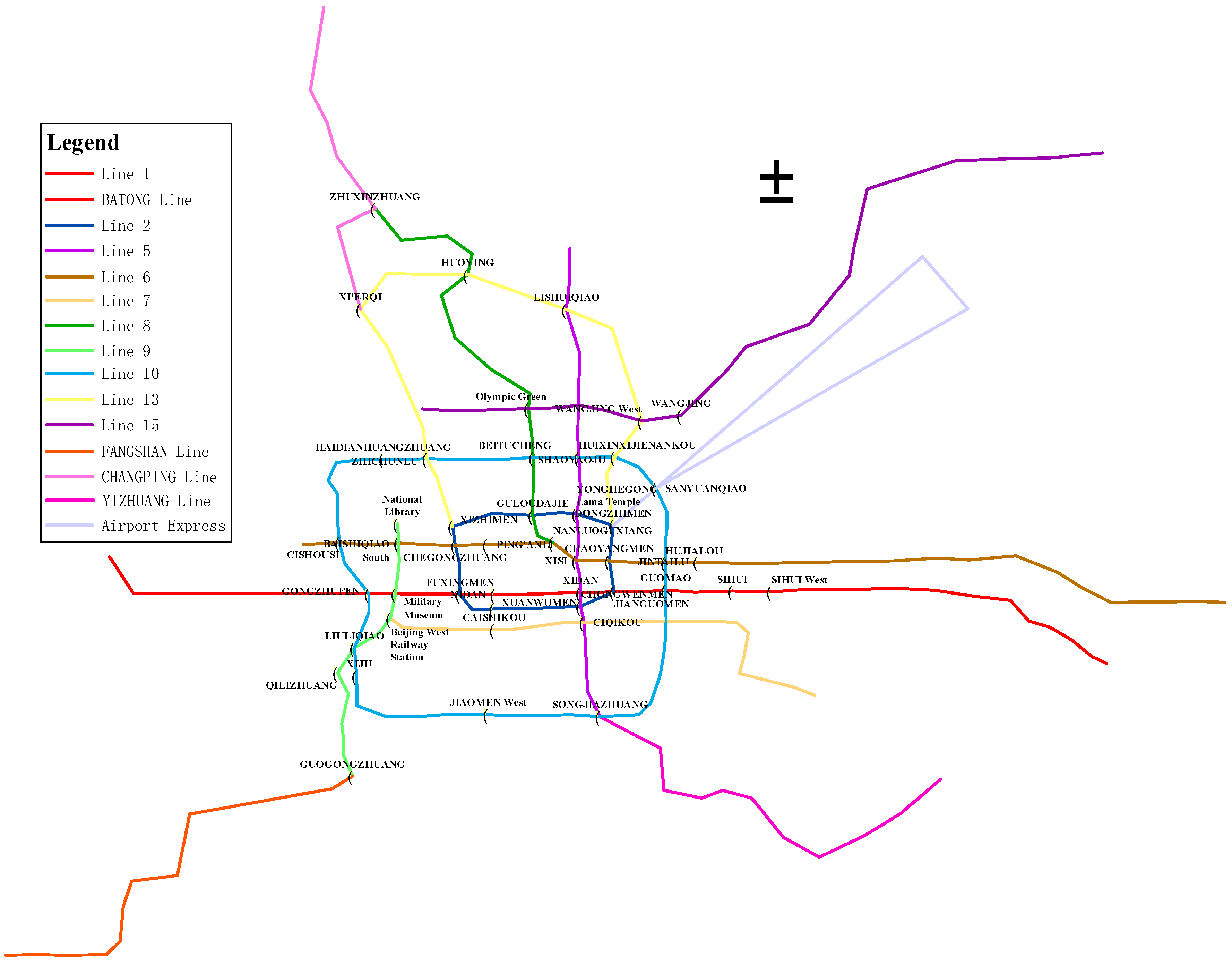
As an international city, Beijing reached a population of 21.542 million by the end of 2018, which means there is a huge demand for public transportation. This paper took the Beijing metro system as a study object, and the experiment data came from the dayparting passenger flow of 47 metro stations and daily passenger flow of 15 metro lines in 2015 (Figure 1).
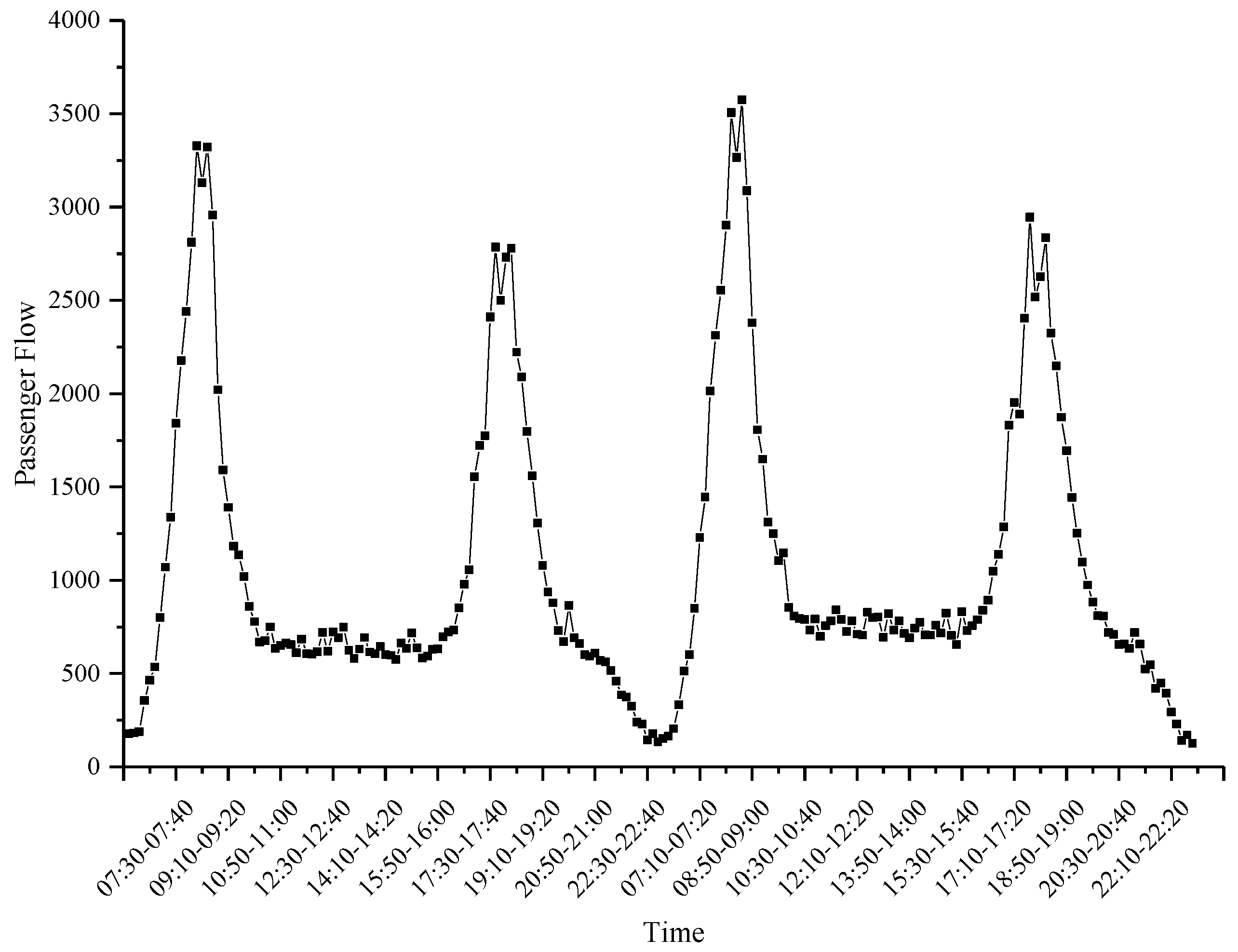
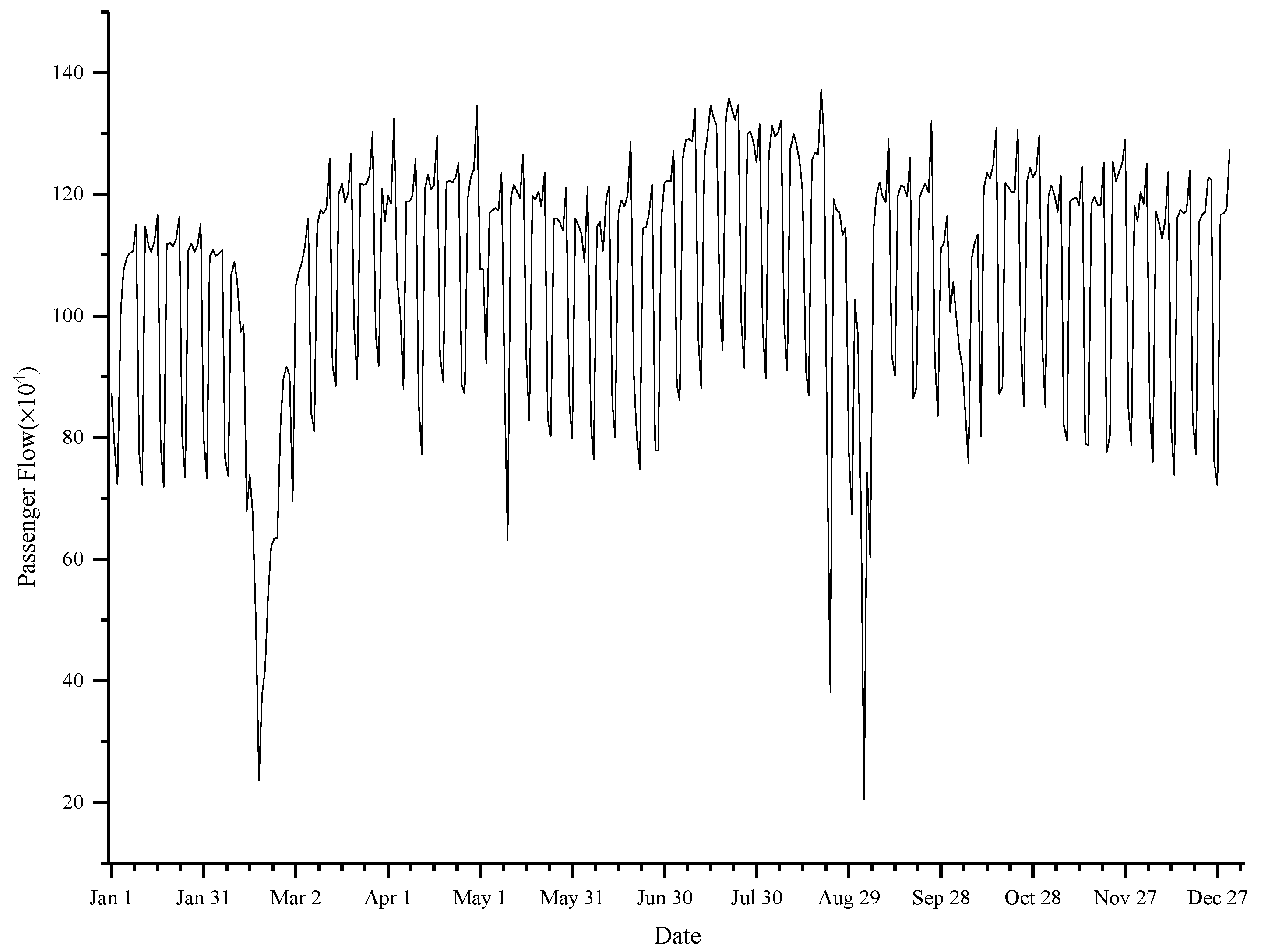
The dayparting passenger flows of metro stations for experiments were a time series at 10-min intervals. In order to train the network with complete knowledge of the nonlinear distribution of dayparting passenger flow, the combination of the passenger flows on 3 March 2015 and on 10 March 2015 (Figure 2, taking XIZHIMEN Station as an example) were input into it. These two days were the Tuesday from the adjacent weeks, which were not holidays or major event days; as such, the dayparting passenger flow of these two days basically conformed to the same distribution law. In addition, passenger flow during the two peaks (7:00–9:30 and 17:00–19:30) accounted for more than 50% of the total daily passenger flow in a single day. Observing the daily passenger flow of the Beijing metro line in 2015 (Figure 3, taking Line 1 as an example), the passenger flow changed periodically, suddenly reducing or surging during the holidays, particularly during the Spring Festival in February.
2.2. Methods
2.2.1. LSTM NN
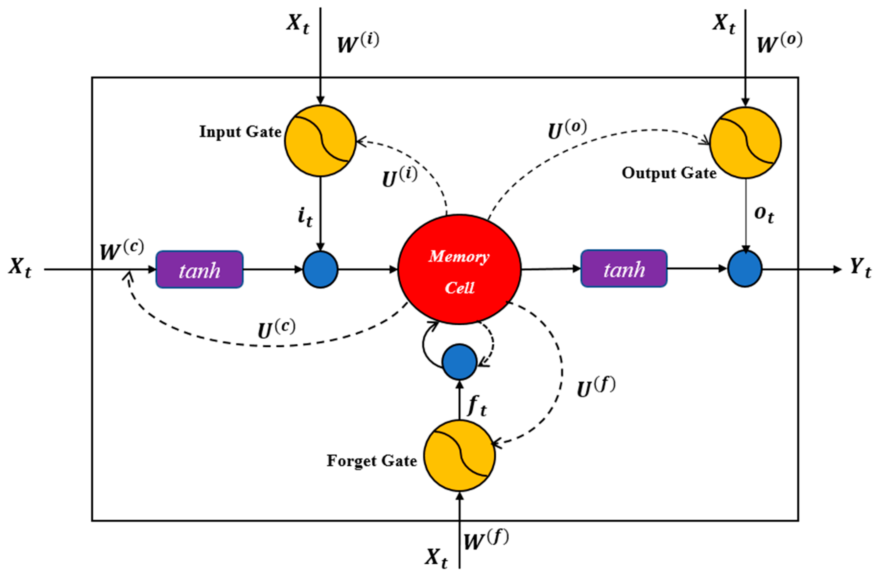
The LSTM NN has long short-term memory capability compared with other RNNs due to its unique network structure. This network consists of an input layer, an output layer, and a recursive hidden layer. The core of the recursive hidden layer is a memory block (Figure 4) [21].
The center of the memory block is the memory cell. In addition, the memory block includes three information control parts: Input gate, forget gate and output gate. The input of the memory block is preprocessed historical passenger flow time series , and the output is predicted passenger flow time series . represents the current prediction period. Using the LSTM NN to predict future passenger flow does not require commanding the network to trace back some time steps. The input time series is iteratively calculated in the memory block, and different information is controlled through different gates. The LSTM NN memory block can capture long and short-term complex connections within a time series. represents the current state of the memory cell. represents the previous state of the memory cell. The dashed lines represent the combination with . Blue nodes represent multiplication. The iterative calculations and information processes in the memory block are represented by the following set of expressions:
where , , and represent the output of three gates, respectively. represents new state of memory cell, and represents the final state of memory cell. , , , , , , and are all weight matrixes. , , and are all bias vectors. denotes Hadamard product, denotes sigmoid function, and tanh is a kind of activation functions.
2.2.2. CNN
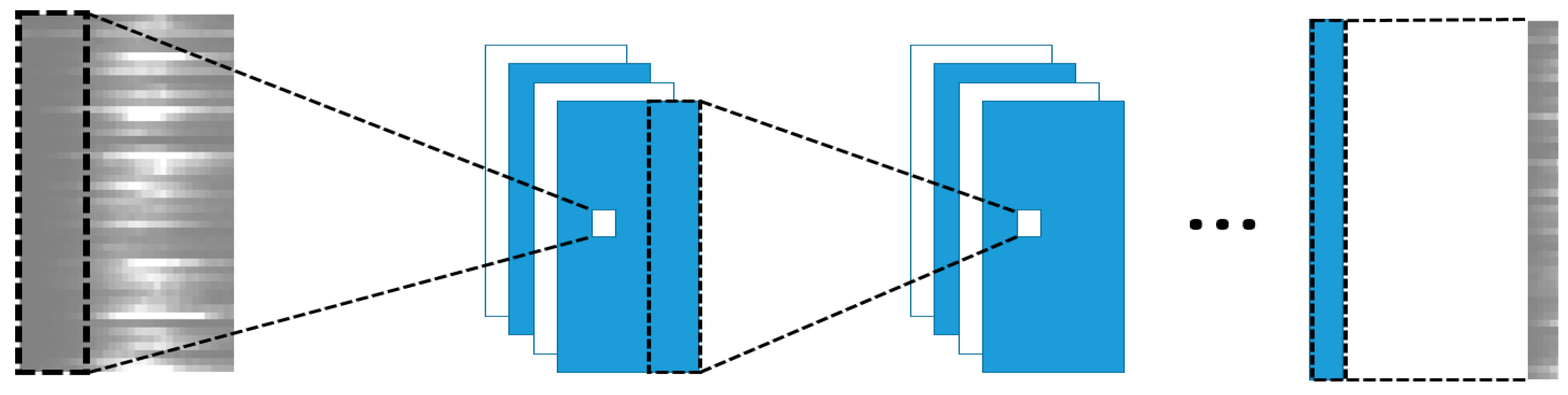
The CNN has shown a strong learning ability and a wide application in image recognition with its unique ability to extract key features from images [30]. The multi-station or multi-line passenger flow spatiotemporal series studied in this paper are essentially two-dimensional matrixes, which can be regarded as single-channel two-dimensional images, so an end-to-end CNN was constructed for the passenger flow spatiotemporal series (Figure 5).
The CNN consists of an input layer, multiple convolutional layers, and an output layer. Feature extraction is performed by convolution filters (also called convolution kernels) in convolutional layers. A convolution filter extracts a feature from the current layer, and then the extracted features are further combined into higher-level and more abstract features, so each convolution filter converts low-level features into high-level features. Using to represent a convolution filter, the filter output is represented as:
where m and n represent two dimensions of the filter. represents the value of the filter input matrix at the e and f positions in the row and column. represents the coefficients of the convolution filter at the e and f positions in the row and column.
Each convolutional layer of the CNN also needs an ReLU (Rectified Linear Unit) function (a kind of activation function) to convert the output of each layer into a manageable, scaled data range, which is beneficial for the training model. Moreover, the combination of ReLU functions can also simulate complex nonlinear functions, which make the CNN have a powerful data processing capability for a complex training set. The ReLU function is expressed as:
When the CNN trains and predicts the two-dimensional matrix of spatiotemporal data, it is generally necessary to use the correlations between stations or lines to specifically arrange the positions of stations or lines in the two-dimensional matrix and then use the standard convolution kernel to extract features. The standard convolution kernel is locally convoluted. However, the spatial correlations between stations or lines in reality are global, so the use of standard convolution kernels has significant limitations. Therefore, this paper adopted convolution kernels with long-shapes and performed full convolution on the spatial dimension of the two-dimensional matrix of the input spatiotemporal data, which made full use of the spatial correlations between stations or lines. The network also cancelled the pooling layer, using the batch normalization and nonlinear ReLU function after each convolutional layer, as well as the output layer.
2.2.3. Methods of Network Training
In the prediction experiments of dayparting passenger flow of metro stations using the LSTM NN, the data of joint passenger flow from 06:00 on 3 March to 17:00 on 10 March were taken as the training set, and the data of joint passenger flow from 17:00 to 23:00 on 10 March were taken as the test set. Because the input and output data were single time series, the number of input and output layer was set to 1. The nodes of hidden layer were set to 50 units, the training epochs were set to 600, gradient threshold was 1, initial learning rate was 0.05, and the learning rate drop was set after 300 epochs by multiplying by a factor of 0.1. In the daily passenger flow prediction experiments of metro lines using the LSTM NN, the daily passenger flow in whole year of 2015 was taken as the training set, and the daily passenger flow of January–February in 2016 was taken as the test set. The number of input and output layers was set to 1, the hidden layer had 100 units, the training epochs had 500, gradient threshold was 1, initial learning rate was 0.05, and the learning rate drop was set after 250 epochs by multiplying by a factor of 0.1.
The CNN proposed in this paper was a full convolution network and finally output the predicted passenger flow of each station and line directly. In the experiments of dayparting passenger flow prediction of metro stations using the CNN, the data of dayparting passenger flow on whole day of 3 March were taken as the training set, and the data of dayparting passenger flow on whole day of 10 March were taken the test set. A full convolutional network with six convolutional layers was constructed for the spatiotemporal data of 47 stations. The first three convolution kernels were (47, 47, 3), with the first three paddings being 1 and the last convolution kernel being (47, 47, 1). In the experiments of the daily passenger flow prediction of metro lines using the CNN, the daily passenger flow in whole year of 2015 was taken as the training set, and the daily passenger flow of January–February in 2016 was taken as the test set. A full convolutional network with six convolutional layers was constructed for the spatiotemporal data of 15 lines. The first three convolution kernels were (15, 15, 3), with the first three paddings being 1 and the last convolution kernel being (15, 15, 1).
Both networks used the mean square error (MSE) as the loss function. All experiments evaluated the prediction performance by three criteria: Mean absolute error (MAE), mean relative error (MRE) and root mean square error (RMSE).
3. Results
3.1. Dayparting Passenger Flow Prediction of Metro Stations Using LSTM NN
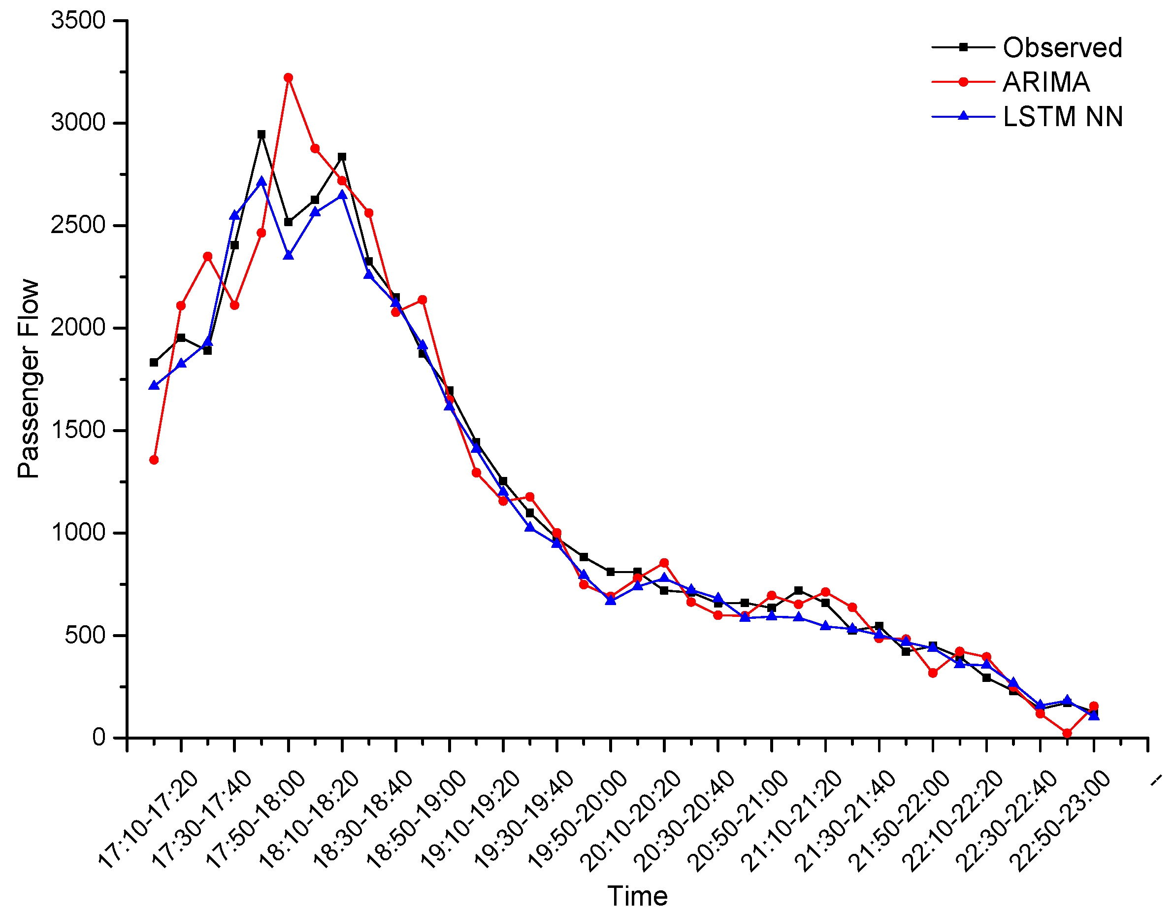
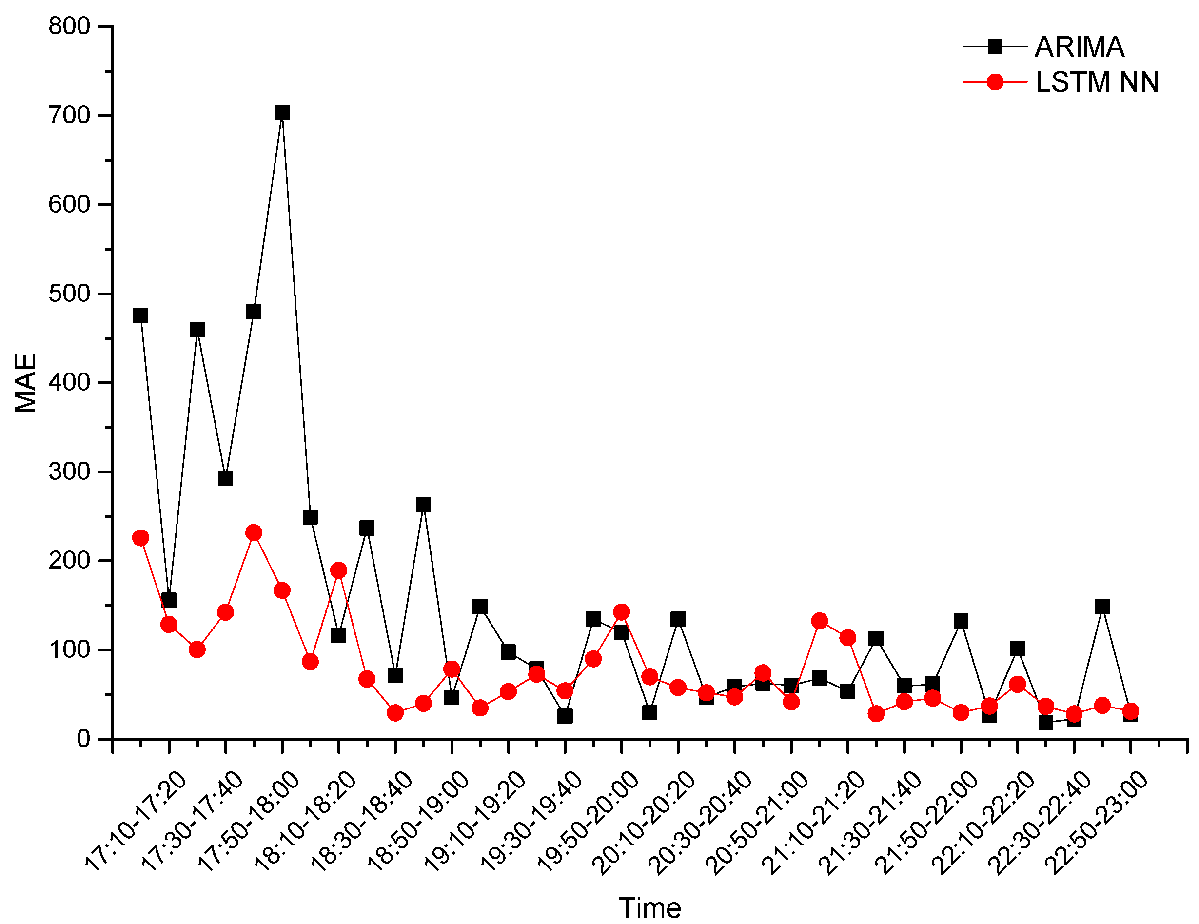
In order to avoid the error caused by the random gradient during network training, we carried out three repeated experiments. For XIZHIMEN Station, the prediction performance for the evening-peak (17:00–19:30) and the full-time (17:00–23:00) is shown in Table 1. Using ARIMA (2, 2, 3) as the contrast experiment, the prediction performances of two methods are shown in Table 2, and the predicted values of the two methods (the LSTM NN took three experiments’ averages) were compared with the observed values, as shown in Figure 6. It can be seen that the prediction accuracy of the LSTM NN was much higher than that of ARIMA, regardless of the evening-peak or full-time, especially in the prediction of peak shape. Comparing the dayparting MAE of two methods (the LSTM NN took three experiments’ averages) (Figure 7), the dayparting MAE of ARIMA fluctuated sharply during the evening-peak, while the dayparting MAE of the LSTM NN remained low throughout the full-time, which indicates that the LSTM NN is highly adaptable to extremely changing data. The MRE of the LSTM NN remained within 10%, regardless of the evening-peak or full time, indicating that the LSTM NN has both long-term and short-term prediction capabilities.
In order to test the applicability of the LSTM NN, 24 other Beijing metro stations were selected for experiments, with ARIMA as the contrast. The prediction performances of two methods for 25 stations are shown in Table 3. In comparison, the prediction accuracy of the LSTM NN decreased when it was applied to 25 metro stations, but its accuracy was still better than those of ARIMA. In addition, the LSTM NN did not require the pre-verification of time series stationarity, eliminating the tedious process of the smoothing and stationarity tests.
3.2. Daily Passenger Flow Prediction of Metro Lines Using LSTM NN
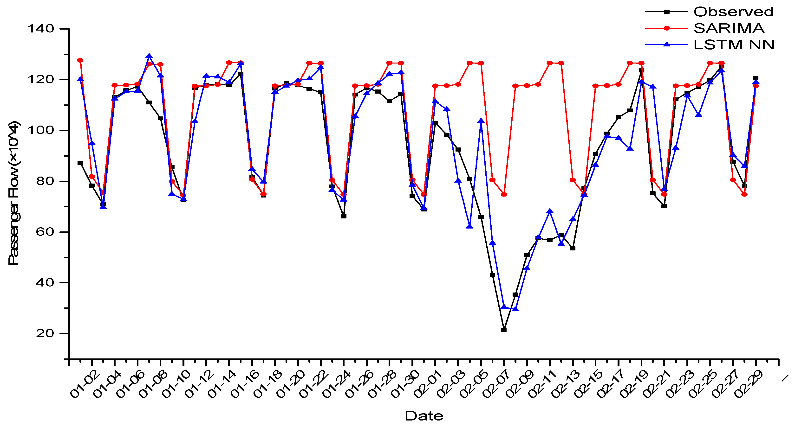
The prediction performance in Beijing metro Line 1 is shown in Table 4. Similarly, in order to set up a contrast experiment, SARIMA (1, 0, 4) (1, 1, 1) was used to model the training set and predict the test set, and the prediction performances of two methods are shown in Table 5. The predicted values (the LSTM NN took three experiments’ averages) were compared with the observed values, as shown in Figure 8. It was proved that the fitting expression of SARIMA was too simple, so the fitting process was greatly influenced by periodicity. SARIMA also had little response to extreme changes in the data. Therefore, it was difficult for SARIMA to predict passenger flow during the holidays. In contrast, in addition to accurately predicting the periodic distribution of daily passenger flow, the LSTM NN also performed well in predicting passenger flow during holidays.
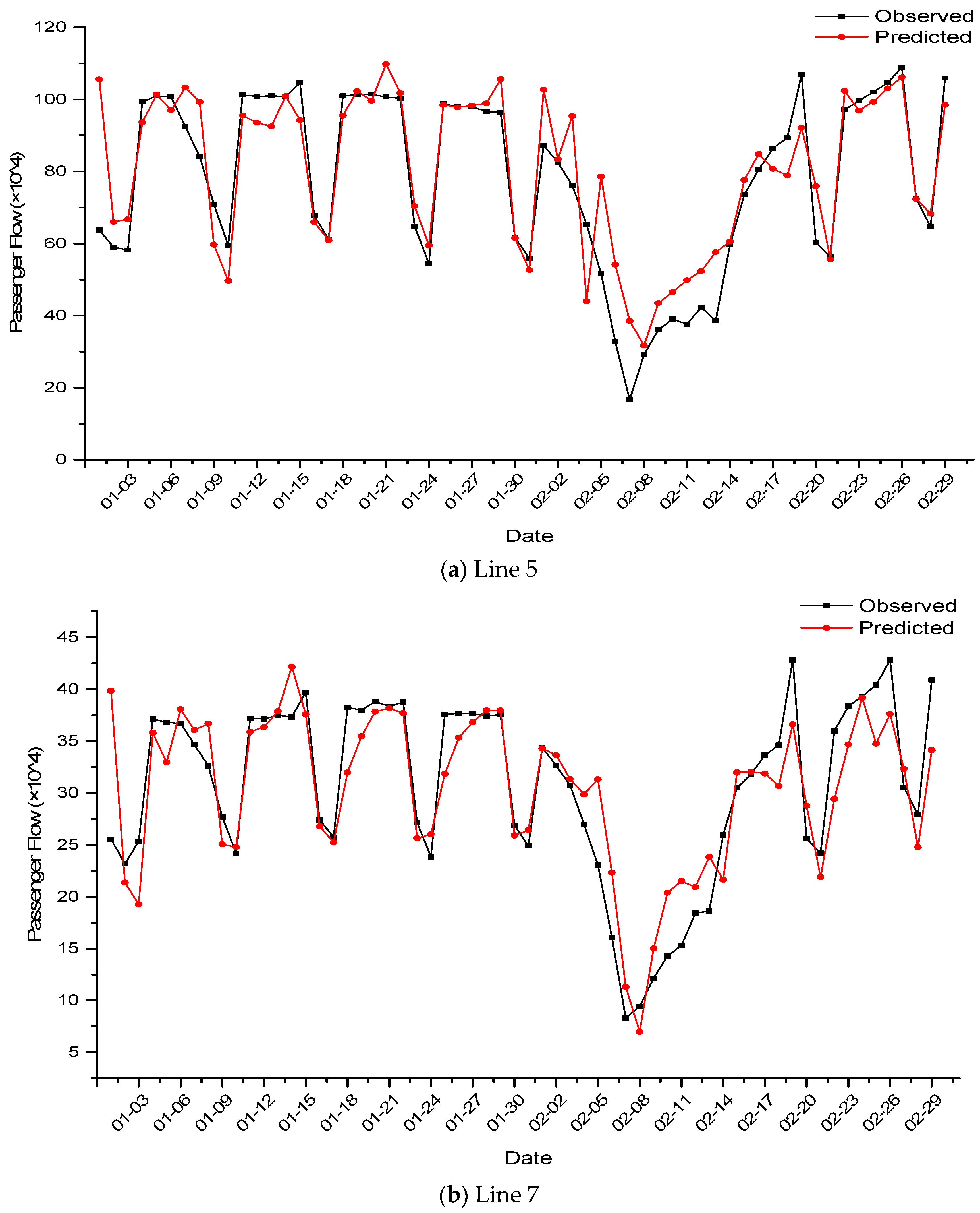
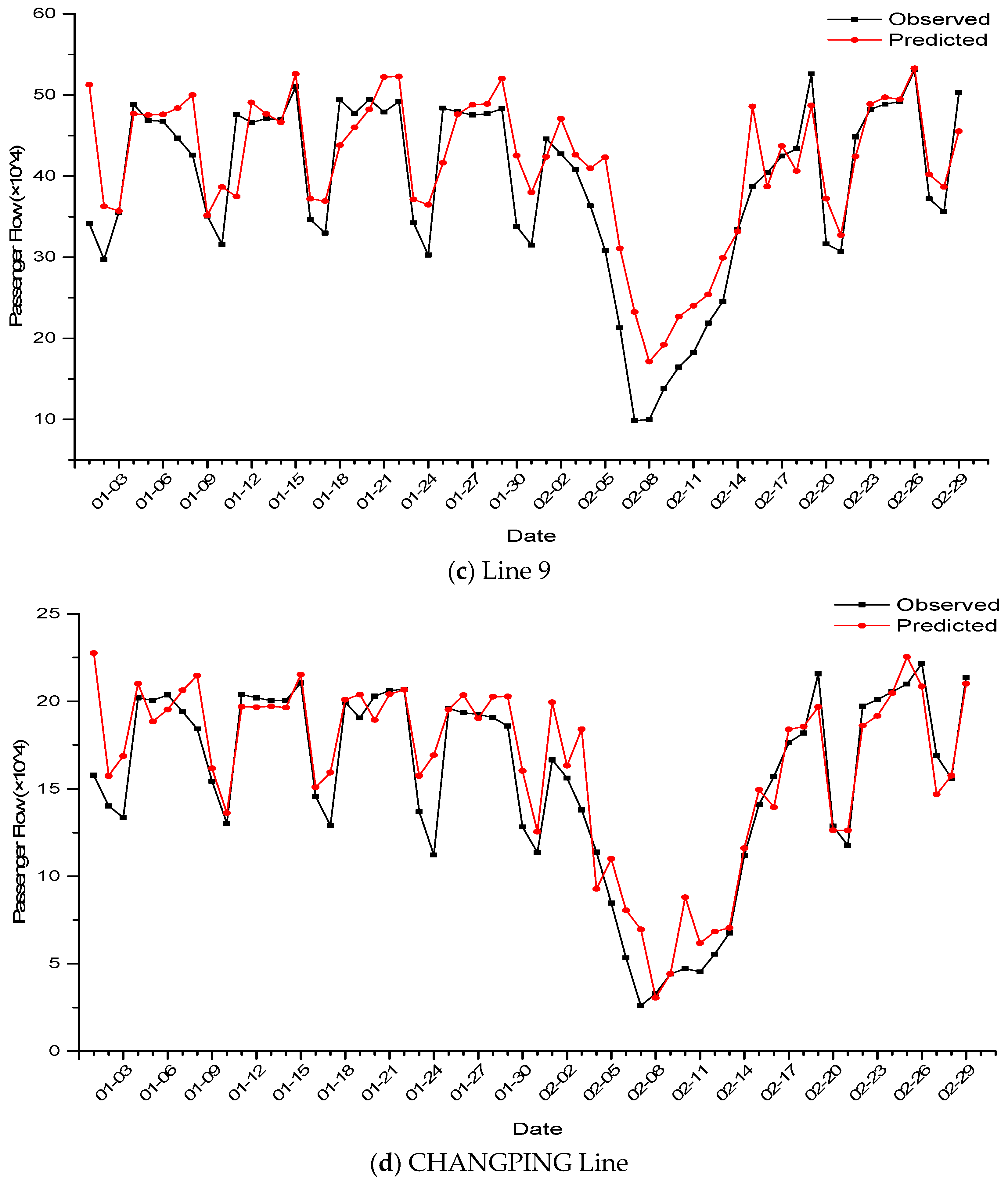
The constructed LSTM NN was applied to the daily passenger flow prediction experiments of 14 other lines. The prediction performance for all 15 lines is shown in Table 6. Figure 9 shows the LSTM NN prediction results of daily passenger flow in Line 5, Line 7, Line 9 and the CHANGPING Line. As seen in Table 6, the LSTM NN could adapt well in the case of the daily passenger flow being disturbed by holidays, obtaining good prediction accuracy.
3.3. Dayparting Passenger Flow Prediction of Metro Stations Using CNN
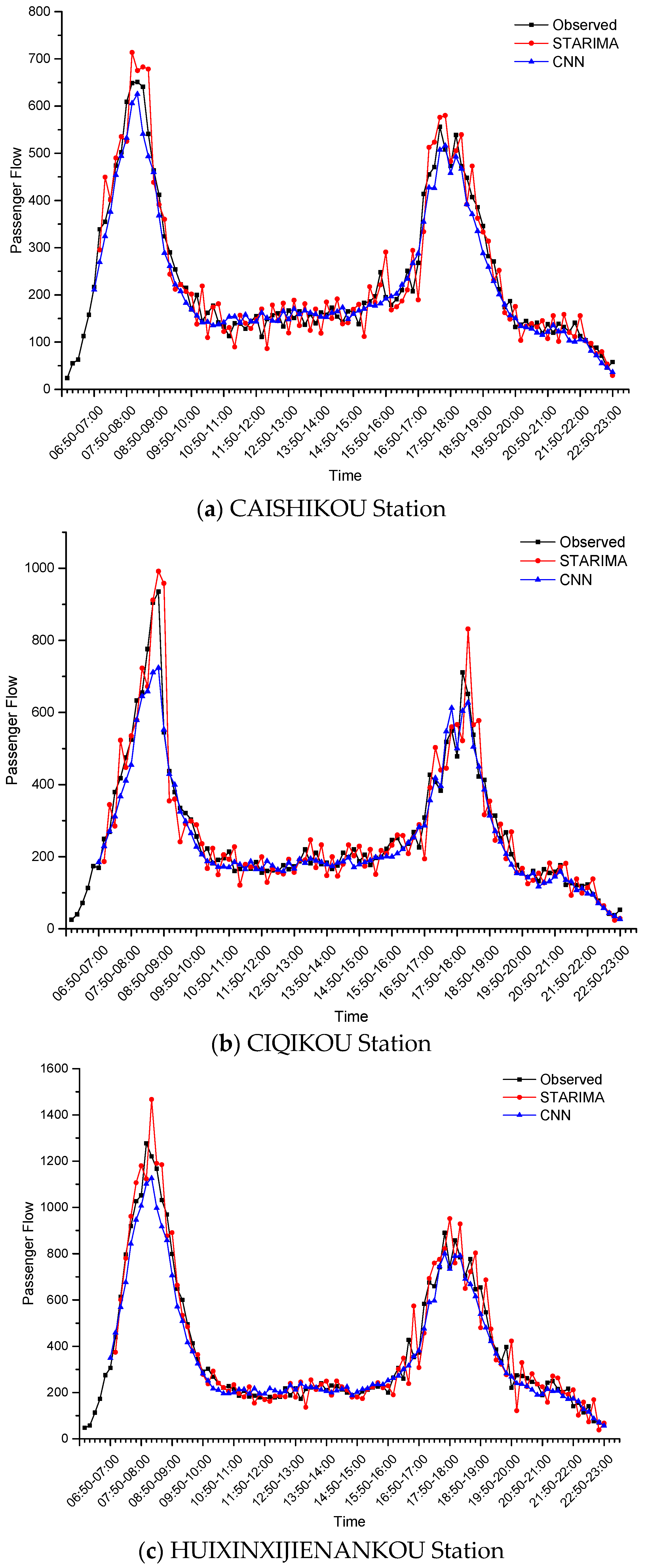
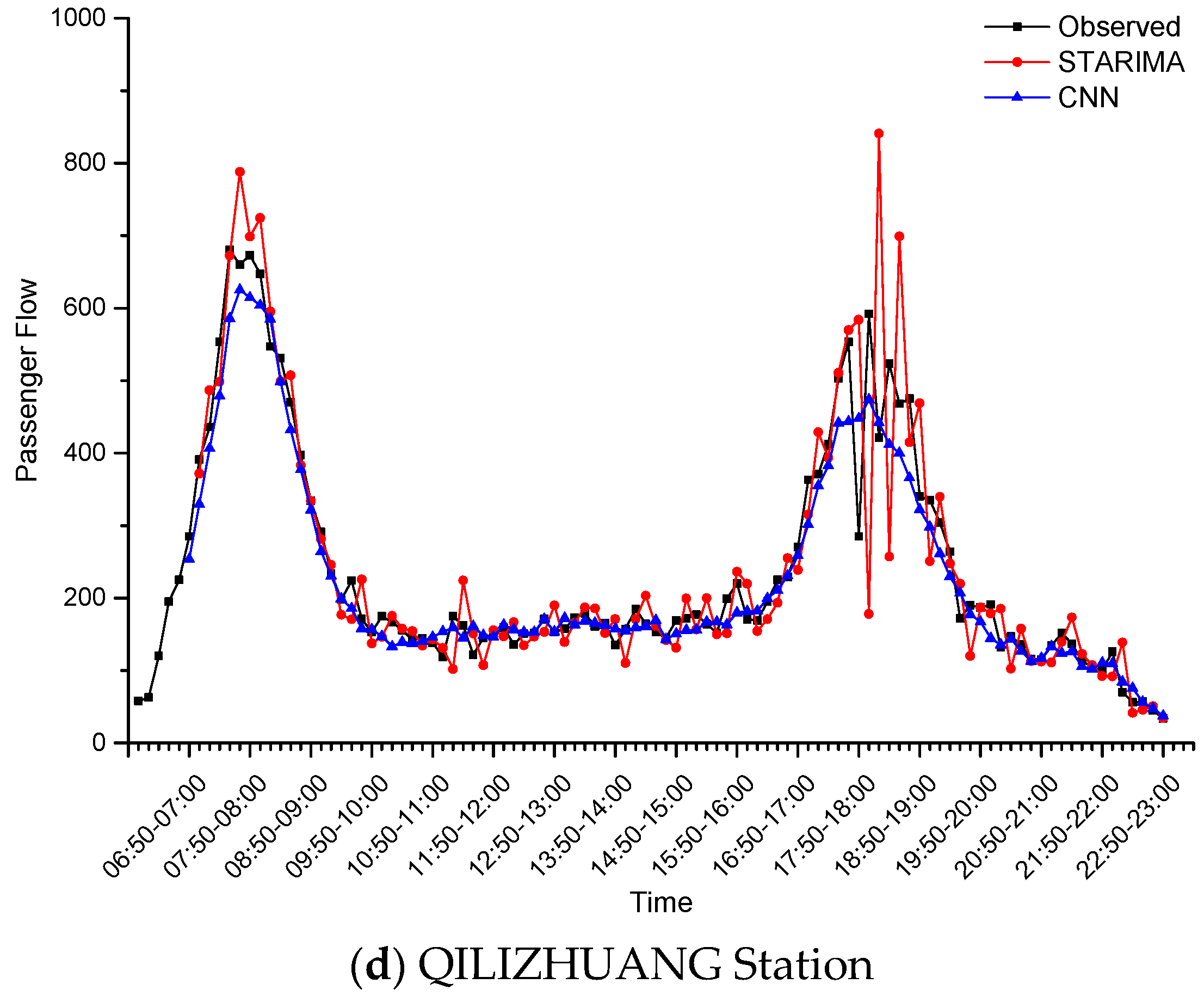
Taking STARIMA as the contrast experiment, the prediction performances of the passenger flow for 47 stations by the two methods are shown in Table 7. Compared with STARIMA, the MAE, MRE and RMSE of the CNN decreased by 24.62%, 29.43% and 27.86%, respectively. Taking CAISHIKOU Station, CIQIKOU Station, HUIXINXIJIENANKOU Station and QILIZHUANG Station as examples, the prediction results of the two methods on the observed values are shown in Figure 10. Though the CNN used less historical data, it obtained better performance than STARIMA. STARIMA was affected by the random fluctuation of passenger flow, and its predicted values deviated from the normal range. The CNN could predict smoothly, even if it faced the fluctuation data, indicating that the CNN is more robust to noise interference.
3.4. Daily Passenger Flow Prediction of Metro Lines Using CNN
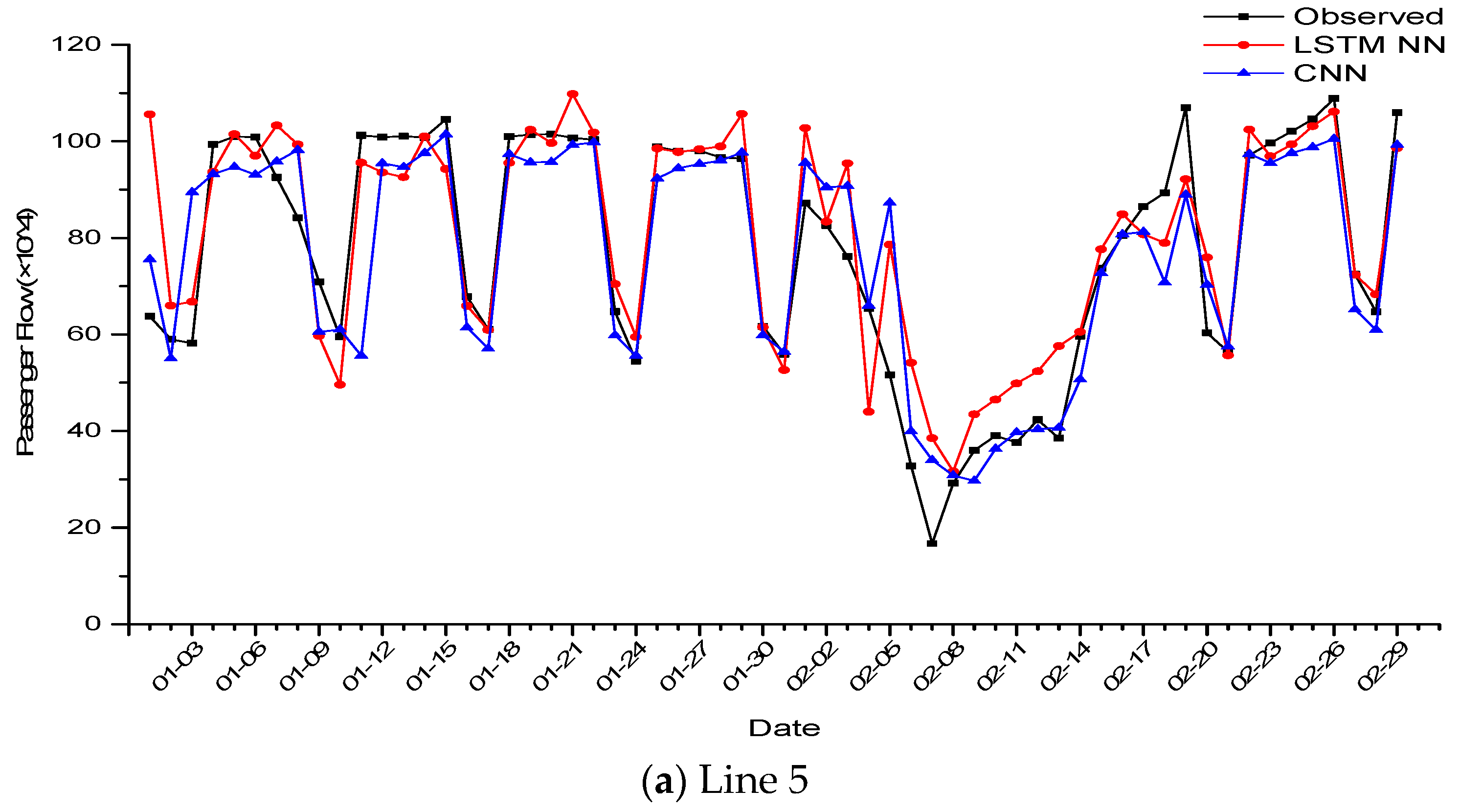
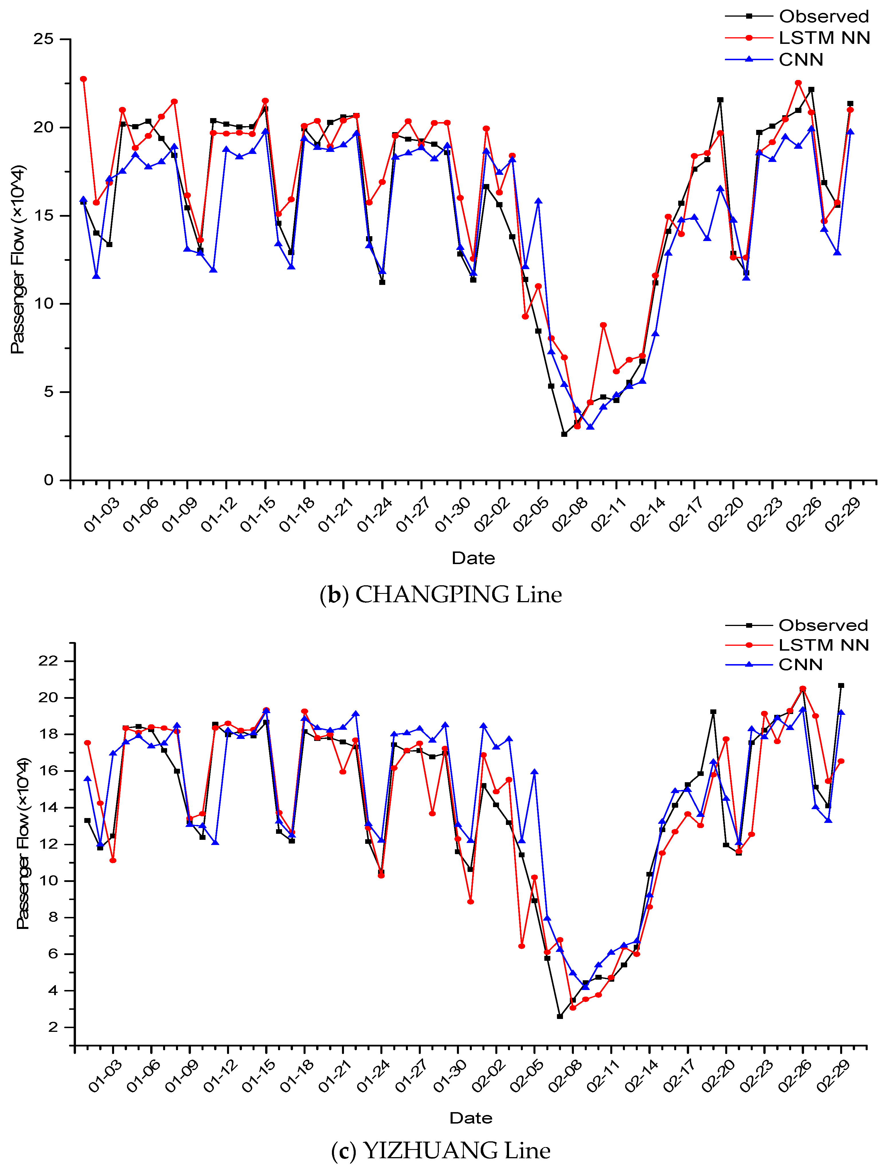
The training set and the test set of the CNN were the same as those of the LSTM NN in experiments of daily passenger flow prediction of metro lines, so we compared prediction results of these two methods. The prediction performances are shown in Table 8. Compared with the LSTM NN, the MAE and RMSE of the CNN were slightly lower, and the MRE of the CNN was slightly higher. However, the differences from the three criteria between two methods were small, indicating that their prediction accuracies were comparable. However, the CNN took the passenger flow of 15 lines as a whole two-dimensional matrix for training, while the LSTM NN constructed in this paper needed separate training for different lines. Taking Line 5, the CHANGPING Line and the YIZHUANG Line as examples, the prediction results of the two methods on the observed values are shown in Figure 11.
4. Discussion and Conclusions
The LSTM NN and the CNN are two popular deep learning methods. While the former’s unique structure of memory cell can capture the long short-term dependencies of time series, the latter has a powerful extraction ability over key image features. According to our studies, the main findings and conclusions are as follows:
- (1)
- When the LSTM NN predicts the dayparting passenger flow of metro stations, the MRE of evening-peak and full-time can remain within 10%, which are much lower than ARIMA. In addition, the superiority of predicting the peak shape is particularly obvious, explaining that the LSTM NN is highly adaptable to extremely changing data and less limited to the prediction term span.
- (2)
- When the LSTM NN predicts the daily passenger flow of metro lines, it overcomes the shortcoming of SARIMA, which has weak responses to dramatic changes in the training set due to the influence of overall periodicity. Hence, the LSTM NN achieves good prediction accuracy during both non-holiday and holidays.
- (3)
- When the CNN predicts the dayparting passenger flow of metro stations, the MAE, MRE and RMSE of the CNN decreased by 24.62%, 29.43%, and 27.86%, respectively, compared with STARIMA, which proves that CNN is less affected by the random fluctuation of passenger flow and has a stronger robustness.
- (4)
- When the CNN predicts the daily passenger flow of metro lines, its prediction accuracy is comparable to that of the LSTM NN. Like the LSTM NN, the CNN has long short-term memory capabilities. Both methods can capture the overall periodicity and dramatic changes of passenger flow, but both will ignore the data shack that lasts too short as abnormal noise.
Based on the above experimental findings, we can prove that the LSTM NN and the CNN can both accurately predict long short-term passenger flow of urban rail transit. They also have good data adaptability and robustness. However, it is difficult for these two networks to capture the transient fluctuation of the passenger flow caused by external disturbance, as this can only be done through learning from the spatiotemporal series themselves. Therefore, in future work, it is necessary to input some prior knowledge outside the spatiotemporal series into the networks to improve prediction results.
Author Contributions
S.Z. principally conceived the idea for the study and was responsible for project administration. Z.X., J.Z., D.S. and Q.H. were responsible for preprocessing all the data and setting up experiments. Z.X. and S.Z. wrote the initial draft of the manuscript and were responsible for revising and improving of the manuscript according to reviewers’ comments.
Funding
This research was funded in part by the National Key R & D Program of China (2016YFC0802500), the Independent Scientific Research Project of the Beijing Research Center of Urban Systems Engineering (2019C013), and the National Natural Science Foundation of China (41471338).
Acknowledgments
We also appreciate support for this paper from the Beijing Key Laboratory of Operation Safety of Gas, Heating, and Underground Pipelines.
Conflicts of Interest
The authors declare no conflict of interest.
References
- Leng, B.; Zeng, J.; Xiong, Z.; Lv, W.; Wan, Y. Probability tree based passenger flow prediction and its application to the Beijing subway system. Front. Comput. Sci. 2013, 7, 195–203. [Google Scholar] [CrossRef]
- Fang, Z.; Yang, X.; Xu, Y.; Shaw, S.-L.; Yin, L. Spatiotemporal model for assessing the stability of urban human convergence and divergence patterns. Int. J. Geogr. Inf. Sci. 2017, 31, 2119–2141. [Google Scholar] [CrossRef]
- Sun, Y.; Leng, B.; Guan, W. A novel wavelet-SVM short-time passenger flow prediction in Beijing subway system. Neurocomputing 2015, 166, 109–121. [Google Scholar] [CrossRef]
- Smith, B.L.; Demetsky, M.J. Traffic Flow Forecasting: Comparison of Modeling Approaches. J. Transp. Eng. 1997, 123, 261–266. [Google Scholar] [CrossRef]
- Williams, B.M.; Durvasula, P.K.; Brown, D.E. Urban Freeway Traffic Flow Prediction: Application of Seasonal Autoregressive Integrated Moving Average and Exponential Smoothing Models. Transp. Res. Rec. J. Transp. Res. Board 1998, 1644, 132–141. [Google Scholar] [CrossRef]
- Xiong, Z.; Zhong, S.; Song, D.; Yu, Z.; Huang, Q. A method of fitting urban rail transit passenger flow time series. China Saf. Sci. J. 2018, 28, 35–41. [Google Scholar]
- Ahmed, M.S.; Cook, A.R. Analysis of Freeway Traffic Time-Series Data by Using Box-Jenkins Techniques; Transportation Research Board: Washington, DC, USA, 1979. [Google Scholar]
- Nihan, N.L.; Holmesland, K.O. Use of the box and Jenkins time series technique in traffic forecasting. Transportation 1980, 9, 125–143. [Google Scholar] [CrossRef]
- Kumar, S.V.; Vanajakshi, L. Short-term traffic flow prediction using seasonal ARIMA model with limited input data. Eur. Transp. Res. Rev. 2015, 7, 21. [Google Scholar] [CrossRef]
- Kamarianakis, Y.; Prastacos, P. Space-time modeling of traffic flow. Comput. Geosci. 2005, 31, 119–133. [Google Scholar] [CrossRef]
- Lin, W.-H. A Gaussian maximum likelihood formulation for short-term forecasting of traffic flow. In Proceedings of the ITSC 2001, 2001 IEEE Intelligent Transportation Systems, Proceedings (Cat. No. 01TH8585), Oakland, CA, USA, 25–29 August 2001; pp. 150–155. [Google Scholar]
- Smith, B.L.; Williams, B.M.; Oswald, R.K. Comparison of parametric and nonparametric models for traffic flow forecasting. Transp. Res. Part C Emerg. Technol. 2002, 10, 303–321. [Google Scholar] [CrossRef]
- Okutani, I.; Stephanedes, Y.J. Dynamic prediction of traffic volume through Kalman filtering theory. Transp. Res. Part B Methodol. 1984, 18, 1–11. [Google Scholar] [CrossRef]
- Sun, S.; Zhang, C.; Yu, G. A Bayesian Network Approach to Traffic Flow Forecasting. IEEE Trans. Intell. Transp. Syst. 2006, 7, 124–132. [Google Scholar] [CrossRef]
- Chen, H.; Grant-Muller, S.; Mussone, L.; Montgomery, F. A Study of Hybrid Neural Network Approaches and the Effects of Missing Data on Traffic Forecasting. Neural Comput. Appl. 2001, 10, 277–286. [Google Scholar] [CrossRef]
- Xie, Y.; Zhang, Y.; Ye, Z. Short-Term Traffic Volume Forecasting Using Kalman Filter with Discrete Wavelet Decomposition. Comput. Civ. Infrastruct. Eng. 2007, 22, 326–334. [Google Scholar] [CrossRef]
- Hu, J.; Zong, C.; Song, J.; Zhang, Z.; Ren, J. An applicable short-term traffic flow forecasting method based on chaotic theory. In Proceedings of the 2003 IEEE International Conference on Intelligent Transportation Systems, Shanghai, China, 12–15 October 2003; pp. 608–613. [Google Scholar]
- Wu, C.-H.; Ho, J.-M.; Lee, D. Travel-Time Prediction With Support Vector Regression. IEEE Trans. Intell. Transp. Syst. 2004, 5, 276–281. [Google Scholar] [CrossRef]
- Ma, X.; Tao, Z.; Wang, Y.; Yu, H.; Wang, Y. Long short-term memory neural network for traffic speed prediction using remote microwave sensor data. Transp. Res. Part C Emerg. Technol. 2015, 54, 187–197. [Google Scholar] [CrossRef]
- Zhong, S.; Yao, G.; Zhu, W. A CPS-enhanced Subway Operations Safety System Based on the Short-term Prediction of the Passenger Flow. In Leveraging Data Techniques for Cyber-Physical Systems; Springer: Berlin/Heidelberg, Germany, in press.
- Zhao, Z.; Chen, W.; Wu, X.; Chen, P.C.Y.; Liu, J. LSTM network: A deep learning approach for short-term traffic forecast. IET Intell. Transp. Syst. 2017, 11, 68–75. [Google Scholar] [CrossRef]
- Schalkoff, R.J. Artificial Neural Networks; McGraw-Hill: New York, NY, USA, 1997; Volume 1. [Google Scholar]
- Hua, J.; Faghri, A. Apphcations of artificial neural networks to intelligent vehicle-highway systems. Transp. Res. Rec. 1994, 1453, 83. [Google Scholar]
- Park, D.; Rilett, L.R. Forecasting Freeway Link Travel Times with a Multilayer Feedforward Neural Network. Comput. Civ. Infrastruct. Eng. 1999, 14, 357–367. [Google Scholar] [CrossRef]
- Park, B.; Messer, C.J.; Urbanik, T.; Ii, T.U. Short-Term Freeway Traffic Volume Forecasting Using Radial Basis Function Neural Network. Transp. Res. Rec. J. Transp. Res. Board 1998, 1651, 39–47. [Google Scholar] [CrossRef]
- Rilett, L.R.; Park, D.; Han, G. Spectral Basis Neural Networks for Real-Time Travel Time Forecasting. J. Transp. Eng. 1999, 125, 515–523. [Google Scholar]
- Lingras, P.; Sharma, S.; Zhong, M. Prediction of Recreational Travel Using Genetically Designed Regression and Time-Delay Neural Network Models. Transp. Res. Rec. J. Transp. Res. Board 2002, 1805, 16–24. [Google Scholar] [CrossRef]
- Hochreiter, S.; Schmidhuber, J. Long short-term memory. Neural Comput. 1997, 9, 1735–1780. [Google Scholar] [CrossRef] [PubMed]
- Lin, F.; Xu, Y.; Yang, Y.; Ma, H. A Spatial-Temporal Hybrid Model for Short-Term Traffic Prediction. Math. Probl. Eng. 2019, 2019, 1–12. [Google Scholar] [CrossRef]
- Ma, X.; Dai, Z.; He, Z.; Ma, J.; Wang, Y.; Wang, Y. Learning Traffic as Images: A Deep Convolutional Neural Network for Large-Scale Transportation Network Speed Prediction. Sensors 2017, 17, 818. [Google Scholar] [CrossRef] [PubMed]
Figure 1.
Beijing metro network map.

Figure 2.
Joint passenger flow of XIZHIMEN Station.

Figure 3.
Daily passenger flow of Line 1 in 2015.

Figure 4.
Structure of the memory block of the proposed long short-term memory neural network (LSTM NN).
Figure 4.
Structure of the memory block of the proposed long short-term memory neural network (LSTM NN).

Figure 5.
Structure of the proposed convolutional neural network (CNN).

Figure 6.
Predicted and observed values of two methods at XIZHIMEN Station.

Figure 7.
Dayparting mean absolute error (MAE) of two methods at XIZHIMEN Station.

Figure 8.
Predicted values of two methods and observed values in Line 1.

Figure 9.
The LSTM NN prediction results in Line 5, Line 7, Line 9 and CHANGPING Line. (a) Line 5, (b) Line 7, (c) Line 9, and (d) CHANGPING Line.
Figure 9.
The LSTM NN prediction results in Line 5, Line 7, Line 9 and CHANGPING Line. (a) Line 5, (b) Line 7, (c) Line 9, and (d) CHANGPING Line.


Figure 10.
The CNN prediction results at (a) CAISHIKOU Station, (b) CIQIKOU Station, (c) HUIXINXIJIENANKOU Station, (d) QILIZHUANG Station.
Figure 10.
The CNN prediction results at (a) CAISHIKOU Station, (b) CIQIKOU Station, (c) HUIXINXIJIENANKOU Station, (d) QILIZHUANG Station.


Figure 11.
Prediction results of two methods in (a) Line 5, (b) CHANGPING Line, (c) YIZHUANG Line.


Table 1.
LSTM NN prediction performance at XIZHIMEN Station.
| Test ID | Evening-Peak | Full-Time | ||||
|---|---|---|---|---|---|---|
| MAE | MRE | RMSE | MAE | MRE | RMSE | |
| 1 | 154.211 | 7.08% | 194.872 | 97.843 | 9.84% | 135.966 |
| 2 | 88.649 | 4.53% | 108.202 | 67.991 | 7.81% | 85.828 |
| 3 | 87.299 | 4.20% | 118.454 | 76.523 | 10.74% | 97.941 |
| Average | 110.053 | 5.27% | 140.509 | 80.786 | 9.46% | 106.578 |
Table 2.
Prediction performances of two methods at XIZHIMEN Station.
| Models | Evening-Peak | Full-Time | ||||
|---|---|---|---|---|---|---|
| MAE | MRE | MAE | MRE | MAE | MRE | |
| ARIMA | 258.505 | 12.26% | 318.266 | 149.677 | 15.08% | 215.058 |
| LSTM NN | 110.053 | 5.27% | 140.509 | 80.786 | 9.46% | 106.578 |
Table 3.
Prediction performances of two methods for 25 stations.
| Models | Evening-Peak | Full-Time | ||||
|---|---|---|---|---|---|---|
| MAE | MRE | MAE | MRE | MAE | MRE | |
| ARIMA | 136.954 | 12.72% | 200.340 | 88.580 | 18.32% | 143.020 |
| LSTM NN | 90.220 | 8.74% | 137.948 | 61.060 | 13.76 | 100.228 |
Table 4.
CNN prediction performance in Line 1.
| Test ID | MAE | MRE | RMSE |
|---|---|---|---|
| 1 | 7.836 | 10.30% | 11.731 |
| 2 | 9.212 | 11.57% | 14.321 |
| 3 | 9.874 | 12.86% | 13.768 |
| Average | 8.974 | 11.58% | 13.273 |
Table 5.
Prediction performances of two methods in Line 1.
| Models | MAE | MRE | RMSE |
|---|---|---|---|
| ARIMA | 15.871 | 27.26% | 26.273 |
| LSTM NN | 8.974 | 11.58% | 13.273 |
Table 6.
The LSTM NN prediction performance for 15 lines.
| MAE | MRE | RMSE |
|---|---|---|
| 4.853 | 12.64% | 9.798 |
Table 7.
Prediction performances of two methods for 47 stations.
| Models | MAE | MRE | RMSE |
|---|---|---|---|
| STARIMA | 75.976 | 17.57% | 128.387 |
| CNN | 57.272 | 12.4% | 92.618 |
Table 8.
Prediction performances of two methods for 15 lines.
| Models | MAE | MRE | RMSE |
|---|---|---|---|
| LSTM NN | 4.853 | 12.64% | 9.798 |
| CNN | 4.557 | 13.46% | 8.682 |
© 2019 by the authors. Licensee MDPI, Basel, Switzerland. This article is an open access article distributed under the terms and conditions of the Creative Commons Attribution (CC BY) license (http://creativecommons.org/licenses/by/4.0/).
Share and Cite
MDPI and ACS Style
Xiong, Z.; Zheng, J.; Song, D.; Zhong, S.; Huang, Q. Passenger Flow Prediction of Urban Rail Transit Based on Deep Learning Methods. Smart Cities 2019, 2, 371-387. https://0-doi-org.brum.beds.ac.uk/10.3390/smartcities2030023
AMA Style
Xiong Z, Zheng J, Song D, Zhong S, Huang Q. Passenger Flow Prediction of Urban Rail Transit Based on Deep Learning Methods. Smart Cities. 2019; 2(3):371-387. https://0-doi-org.brum.beds.ac.uk/10.3390/smartcities2030023
Chicago/Turabian StyleXiong, Zhi, Jianchun Zheng, Dunjiang Song, Shaobo Zhong, and Quanyi Huang. 2019. "Passenger Flow Prediction of Urban Rail Transit Based on Deep Learning Methods" Smart Cities 2, no. 3: 371-387. https://0-doi-org.brum.beds.ac.uk/10.3390/smartcities2030023