Zenneck Waves in Decision Agriculture: An Empirical Verification and Application in EM-Based Underground Wireless Power Transfer


Department of Computer and Information Technology, Purdue University, West Lafayette, IN 47907, USA
*
Author to whom correspondence should be addressed.
Smart Cities 2020, 3(2), 308-340; https://0-doi-org.brum.beds.ac.uk/10.3390/smartcities3020017
Submission received: 26 March 2020
/
Revised: 27 April 2020
/
Accepted: 28 April 2020
/
Published: 6 May 2020
(This article belongs to the Special Issue Internet of Things in Digital Agriculture)
Abstract
:In this article, the results of experiments for the observation of Zenneck surface waves in sub GHz frequency range using dipole antennas are presented. Experiments are conducted over three different soils for communications distances of up to 1 m. This empirical analysis confirms the existence of Zenneck waves over the soil surface. Through the power delay profile (PDP) analysis, it has been shown that other subsurface components exhibit rapid decay as compared to the Zenneck waves. A potential application of the Zenneck waves for energy transmission in the area of decision agriculture is explored. Accordingly, a novel wireless through-the-soil power transfer application using Zenneck surface waves in electromagnetic (EM) based wireless underground communications is developed.

1. Introduction
Smart cities are not only the representation of a technological advancement but also represent development in economical, social, and environmental aspects of the world. The popularity of smart cities has increased the global trend of urbanization up to 70% in European and Asian countries [1]. This increase in urbanization has lead to a transformation of most of the rural land to smart cities, decreasing overall arable and agricultural land. However, with a rapidly increasing human population [2], a decrease in land capable of producing food can put unbearable load on existing, scarcely available, world resources. For example, currently, 70% of the world’s water resource is being used to produce food for the world. Therefore, to realize a complete and sustainable smart city ecosystem, it is imperative to shift from traditional agricultural and farming techniques to smart farming techniques. To that end, this work explores the use of Zenneck surface waves [3,4,5,6] to improve the decision agriculture sector [7] of smart cities.
2. Electromagnetic (EM)-Based Wireless Power Transfer in Decision Agriculture
The energy conservation issues are also important in the development of such sensor systems. For prolonged and uninterrupted operation in the soil, these sensor systems should have the ability to harvest energy from the environment as well as be able to wirelessly received power from soil and other aboveground sources (rechargers). This wireless power transfer to these sensing systems can be achieved through the propagation of subsurface radio frequency Transverse Magnetic (TM) mode where soil–air interface serves as a waveguide. The efficiency of this scheme can be increased two-fold by using multiple transmitters on and below the soil–air interface, creating two such modes, hence, maximizing energy transfer using Zenneck waves [8,9,10,11].
Decision agriculture is a data management strategy. It involves collection, processing and analysis of the spatially and temporally variable data. The data can be combined with other existing available information to make the management decision. The purpose of decision agriculture is to increase resource utilization, production efficiency, quality, productivity, sustainability and profitability of the stakeholders involved in an agricultural process.
There are some factors which should be kept in mind while adapting decision agriculture: (1) The lifetime of sensing equipment should be at least five years, (2) Wireless Power Transfer (WPT) methodologies must be adopted to power up the underground sensing equipment for prolonged and sustainable operations, and (3) development of energy efficient sensing equipment. With advancement in the technology, the energy demand of the sensing material has been significantly reduced. However, they still needs an energy source to communicate with the aboveground receivers. Energy harvesting methods reduce the time-consuming, costly and laborious operations of replacing, maintaining, repairing and re-installation of batteries in underground equipment. These operations may also cause disturbance to plants and soil. To that end, energy harvester techniques can be employed in the field. Intermittent energy sources, e.g., solar energy, vibration, thermal, etc., can be used to harvest energy in precision agriculture. However, the performance of wireless RF power transfer for underground environment needs to be tested yet.
In this paper, an underground wireless power transfer approach has been developed using Zenneck waves. The successful realization of the proposed approach will accelerate the agricultural field deployment through extending the lifetime of underground devices.
The contributions of this paper are summarized in the following:
- We have empirically verified the Zenneck waves in wireless underground communications.
- We develop a novel wireless through-the-soil power transfer application using Zenneck surface waves. To the best of our knowledge, this is the first work which considers use of Zenneck waves in EM-based wireless underground communications.
3. Related Work
There are different methods to empower underground devices used in decision agriculture. To that end, this section discusses existing methodologies being used in the literature.
WPT technologies based on EM induction, magnetic resonance and radiation are discussed first. RF power transfer methods use EM waves to transfer energy from an energy source to underground devices. In comparison to induction and resonance-based techniques, EM-based methods have relatively lower attenuation; thus, they are preferred to achieve long distance communication [12]. The underground devices in agriculture normally operate at the power of a few milli-Watts (mW). This lower power is achieved by exploiting the concept of duty cycling. Duty cycling improves the power consumption by reducing the operating time of underground devices by activating them only when they are needed, i.e., when sensing and communication is required. Sleep time can vary from hours to days in a large farm. It depends upon the time of the season (e.g., growing season), climate and irrigation requirement of the farm. Hence, even the power of few micro-Watts (μW) is enough for the agricultural operations [8,13].
Wireless RF power transfer needs an external source of energy. To that end, a power beacon can be developed as a continuous energy source. However, it is very difficult to deploy a fixed and permanent aboveground power beacon in agricultural fields. Therefore, moving agricultural machinery, e.g., tractors, can be used to serve as a moving aboveground energy source where beacons are mounted on them [14]. Moreover, advancement in technologies have enabled use of Unmanned Aerial Vehicles (UAVs) as an energy source mounting beacons, sensing and data collection equipment [15]. Such UAVs are being used to transfer power and information simultaneously. Another important area of investigation is transferring power through soil. An optimal value of sensor depth and distance between the charged devices should be modeled by carefully understanding the trends in signal attenuation in the soil [7]. In [16], authors have presented a detailed survey on existing energy transfer methodologies in over-the-air (OTA) wireless communication systems. Two antenna designs can be used for external power sources: Single and multi-antenna. In single antenna design, energy is transmitted to only one node at any instant of time. However, in multi-antenna, energy is transmitted and directed towards multiple nodes with the help of beamforming techniques.
In the above mentioned methods, sub-surface devices have to interact with the aboveground RF energy sources to fulfill their energy demands. In-situ energy harvesting methods are proposed to completely eliminate this interaction. Therefore, this section discusses the energy transfer methods other than the RF-based sources. Vibrations can be converted to energy using a piezoelectric effect. This can be achieved using electrical circuits and mechanical methods, e.g., mass, spring and damper [17,18]. However, it is very important to achieve a correct vibration frequency to generate energy using this method. As there are multitude diverse pieces of equipment with varying traffic load in the field, different frequencies are generated from these pieces of equipment. To that end, two options can be used: Either using the multiple sensors with different vibration frequencies or a single sensor with a broad range of frequency spectrum [19,20]. The work in [17] applies vibration energy harvesting in corn fields. They use the field equipment, i.e., seeders, harvesters etc., as a vibration source to harvest energy through piezoelectric technology. This study underscores the possibility of vibration energy harvesting in decision agriculture. However, it is still a challenge to provide continuous energy to a multitude of underground sensors to extend their lifetime and to achieve sustainable field operations because this method is not able to fulfill the energy demands of large numbers of underground sensors. Another challenge is the burial depth of the equipment; attenuation increases with the increase in burial depth [21]. Therefore, vibration energy harvesting needs to be developed in the context of underground environment to solve these challenges. Underground power transfer methods require their own specialized protocols and platforms with an extensive field validation in the context of models, power consumption and non-linear efficiency [7]. Then these protocols can be used in combination with the underground channel estimation methods.
Generally, agriculture fields lack ambient RF energy sources, i.e., stray EM waves, which can be utilized to harvest energy for self-sustainable operation of sensor devices [22]. Another harvesting approach is to harvest energy from received communication signals. Two approaches can be adopted for harvesting energy from communication signals: Time sharing and frequency sharing [22]. In time sharing, time slots are divided between the information transfer and RF energy transfer. In frequency sharing, the information signal shares its frequency with the energy harvesters. Beam splitting can also be used to distribute energy using an energy scheduling approach. Such power and information transfer approaches are studied in [12,23,24]. However, these can lower the performance of information communication and need new equipment, thus increasing the deployment cost. A rectenna is a specialized antenna used for energy harvesting which can be used for collection and rectification of the EM waves [22].
In this regard, Zenneck waves can be used for external power transfer for decision agriculture application [25]. These waves are discussed in the next section.
4. Zenneck Waves
A wave traveling in a straight line (neither reflected nor refracted) along the soil surface is known as a Zenneck wave. These waves are also called lateral waves. Another name for the Zenneck wave is “up-over-and-down” waves. These waves are incident on the soil surface with a critical angle . A lateral wave continuously travels along the soil surface until it reaches the receiver (see Figure 1 [26]). Soil attenuation in a lateral wave is limited to the sum of the sender’s and the receiver’s depth. Hence, the communication range is increased in the shallower depth, even if the transmit power is kept the same [27,28,29,30].
There are total of six EM wave components of a Zenneck wave originating from a horizontal electrical dipole. These six components can be divided into two major groups: Electric and magnetic, each having an equal number of components. The three electrical components (referred to as TM in this paper) are cylindrical and are represented by , , and . Magnetic components (referred to as TE in this paper) are represented as , , and . The values of these components are important in the mediums in which they are traveling. The mediums are usually air or dielectric. On applying current to the dipole, the electric components of a Zenneck wave travel, through air, to the observation point = L. A similar electric pulse is reflected in the reverse direction from the dielectric.
TM and TE types of trapped surface waves are generated by the horizontal electric dipole due to the air–dielectric surface of the microstrip. The cut-off frequency of this pulse is much smaller as compared to that of the Direct Wave (DW) pulse. The growth of the Zenneck wave is increased with the increase in radial distance and this growth is relative to the DW pulse. Both DW and Zenneck wave pulses are quite different from each other. An initial pulse generated by superimposing the frequencies from 5 MHz to 50 GHz with a 50 MHz interval is applied to the microstrip.
An electric field is generated by exciting a horizontal electric dipole with Gaussian current pulse. The dipole is placed at the surface of the microstip and the field is generated in an outward direction and consists of a surface-wave pulse traveling with the speed of light in both air and dielectric media. The field moves along the conductor strip and a current is induced in the conductor due to the associated radial electric field. At any given point of the transmission line, all currents induced by the radial field are superimposed and precede the Gaussian current pulse arriving at that point. Thus, the actual pulse at the point is the superposition of the all currents generated from the preceding, arriving and original pulses. This combined pulse is much longer than the original Gaussian pulse. Its shape is determined by the distribution of the electric field in time at a given point. These pulses are estimated using the effective wave number in the spectral domain.
The surface-wave pulse generated by a Gaussian current pulse, at a boundary of two dielectrics, is a derivative of a Gaussian pulse. The direct wave field in the air also propagates as a Gaussian pulse and the surface wave field propagates as a derivative of the Gaussian pulse. When conducting half-space, both pulses are reflected and combine with the direct field producing the final shape of the pulse.
The structure of the microstrip is well suited for the analysis of two different wave propagations because: The air—dielectric boundary is the most suited structure for Zenneck wave propagation or propagation of pulse in the air, and it is important for trapped waves to have a medium with a dielectric layer on a highly conductive plane.
A single broadened pulse is generated from the superposition of two similar and simultaneously arriving pulses. Hence, a trapped wave is combined with the TM component of a Zenneck wave so that the Zenneck wave becomes indistinguishable. The dielectric layer has a very thin electrical layer; therefore, the total thickness of the dielectric layer determines the amplitude of the combined field. The combine pulse is similar to the Zenneck wave along the dielectric half-space.
The surface wave at the ice layer has a negligible amplitude as compared to that of currents in the sea; hence, it can be ignored. Therefore, the sea field is similar to that of the field from the unit dipole at the surface of sea or ice. A bare antenna can be placed on ice with both ends terminated with vertical extension into the sea, hence giving it insulation with two-layered dielectric. Due to lack of formulae, the approximate values are used for wave number and characteristic impedance of the antenna insulated through single dielectric ice. The following properties are revealed after the analysis of field in air and field in dielectric coated media:
- The air—Zenneck wave and the dielectric—Zenneck wave can be combined into a single wave if the electrical length of the wave is small. It can propagate in air and a thin dielectric with a wavenumber.
- For a larger but finite length, a new Zenneck wave is generated along the air–dielectric boundary. This wave is associated with the polarization dn conduction currents in the region in which it is generated. A Zenneck wave is the result of the superposition of these two waves.
5. Zenneck Wave (ZM) Channel Model
5.1. Background
The Wireless Underground Communication (WUC) found its application in many areas, e.g., environmental monitoring, infrastructure monitoring and security monitoring. For environmental monitoring, it is being used in landslide monitoring and precision agriculture, and for infrastructure monitoring, it is being used in natural disaster situations to locate people, preventing leakage. Finally, for security monitoring, it is being used to detect illegal infiltration at borders using hidden underground devices.
WUCs differ from traditional wireless networks in that they use a completely different medium, i.e., soil, to communicate. Soil has not been thought of and investigated as an ideal medium for EM propagation for decades. The primary goal is to achieve long-range communication through soil using low-power devices. Therefore, there is a need to develop a power-efficient solution for communication in an underground environment. However, power-efficient communication in an underground environment faces many challenges and, due to these challenges, there is no detailed wireless channel or protocol development for WUC. To that end, detailed experiments were performed along with the extensive review of existing literature [31,32,33,34,35,36]. The experiments investigate the effect of irregular soil surface and soil texture and moisture, antenna design, burial depth and operating frequency. The experiments showed that soil and antenna properties affect communication. This proves that spatio-temporal environmental factors are related to the communication system. Therefore, it is important to consider these factor for an underground channel.
In this section, we present a Zenneck wave (ZM) channel model which is based on the research work of A. Silva [26]. The main focus of the model is to present a propagation model instead of the antenna problem. The antenna problem is not considered to keep the model simple as there exist many antenna schemes. The model uses directivity of special antennas to estimate the gain. It uses different components such as three wave components (direct wave (DW), reflected wave (RW) and lateral wave (LW) factors), the signal superposition model and the dielectric soil property prediction model. As a result, the model outputs bit rate error (BER) and level of signal attenuation.
The LW component was excluded while performing in-situ experiments and the model was validated from gathered results. Long-range communication can be achieved with the LW component, that too without increasing any power level. For UG nodes, this long range (distance > 10 m) along with the combination of any multi-hop networking solution can eliminate the topology dependency of the UG node on the aboveground nodes [26].
Underground channel characterization is an important task and it can play an important role in the improvement and proliferation of Wireless Underground Sensor Network (WUSN) communication protocols. In contrast to the over-the-air channel, the underground communication channel is highly affected by environmental factors because of the correlation between these factors and the dielectric properties of soil [37,38,39]. In addition to the environmental effect, deployment parameters also affect the communication performance [31,37]. Therefore, while characterizing underground communication channels, it is imperative to consider not only environmental but deployment factors as well.
5.2. Model Components
Underground-to-Underground (UG2UG) communication channels are characterized from analyses of empirical study results given in [31,32,33,34,40,41]. A Zenneck wave (ZW) model is proposed which predicts signal attenuation and bit error rate (BER) in a UG2UG link [26]. Model components are described below [26]:
- Dielectric properties model. This component captures the dielectric properties of the soil. It assumes that volumetric water content (VWC) data is readily available. It also measures soil texture and bulk density to measure the environmental effect on the communication. However, these values are measured only once as no show temporal variations are shown [42]. Hence, the model can measure the soil permittivity and soil conductivity under the frequency range of 300 MHz to 1300 MHz [26].
- Direct wave model. This model is used for predicting attenuation due to the direct wave (DW) component of the signal. It is interesting to note that, although ZW is mainly used in UG2UG communication links, its first two components can also be used in UG2AG and Aboveground-to-Underground (AG2UG) communication links as a future research direction.
- Reflected wave model. This model is used to predict attenuation because of the reflected wave (RW) component of the signal [26].
- Lateral wave model. This model is used for predicting attenuation due to the lateral wave (LW) component of the signal. Lateral wave propagation is also known as up-over-and-down propagation [28].
- Signal superposition model. The final received signal is the result of the superposition of DW, RW and LW wave components. This model measures the overall strength of the transmitted signal for comparison with the overall strength of the received super-positioned signal [26]. If any one of the wave components is affected by the environmental parameters, i.e., burial depth or the inter-node distance, it will effect the overall strength of the signal received at the receiver. Practically, if the power of any one wave component exceeds others by 10 dB, the resultant super-positioned signal will have a negligible effect from other low power wave components. Finally, ZW estimates total signal attenuation and BER as an output [43,44].
5.3. The Model Development Preliminaries
This section discuss the basics of the ZW channel model for UG2UG communication. The following terminology is going to be used for the rest of the paper: denotes burial depth, is horizontal distance between the nodes and is the actual distance between the nodes. All parameters for the sender will have a subscript of s and those related to the receiver will use the subscript r. A reflected wave is a wave which is reflected from some point on the soil surface. The distance between the reflection point on the soil and the sending node is denoted by and, for the receiving node, is denoted by . The incident angel is given by , the reflection angle for normal soil surface is represented as and the reflection angle using Snell’s law of reflection is given as [26].
The three wave components, DW, RW and LW, are shown in Figure 1 [26]. It can be seen that the final signal will be the combination of all three wave components that are traveling on three different paths. The DW attenuation model is the simplest of all models as it only considers attenuation occurring due to soil propagation. The RW attenuation model adds reflection due to soil surface as an additional parameter while estimating attenuation. The signal attenuation occurring because of reflection is highly dependent upon the permittivity of the soil, and , and .
It is shown in [45] that the lateral wave component is dominant at the critical angle . The value of varies from 10° to 20°. is dependent upon the soil and air dielectric properties. The LW model is the most complex component of the ZW model because of the absence of an analytical solution to determine the electric fields of LWs [28,46]. Therefore, the numerical approach presented in [28,47] is used to find the LW contribution in signal attenuation. Finally, the superposition model is used to determine the individual component effect (both positive or negative) on the signal attenuation due to phase and magnitude.
To avoid complexity, antenna orientations are not considered while evaluating the ZW model because using different antenna schemes may cause distortion in the ZW model. Therefore, unique antenna parameters are used for each signal component. These factors will also be given as an input to the ZW model (Section 5.5). However, accuracy should not be compromised while evaluating the model, both empirically and analytically [26].
Another assumption of the model is to use insulated antennas [26]. In practice, this assumption will not effect the operation of small antennas, e.g., Mica2 mote antennas are originally insulated. The model also assumes that antennas are enclosed in some box or container because they can also highly affect the signal. This assumption of node deployment may be changed if the model is used for stratified media. Moreover, non-magnetic soil is used for the model [48].
5.4. UG Radio Wave Components and Modeling
5.4.1. Dielectric Model
The dielectric model is originally taken from [49]. The original dielectric model has a frequency limitation of 300 MHz to 1300 MHz. While it is possible to use different dielectric models with different frequency limitations, existing literature concludes that these frequency ranges are a balanced range for WUC implementations [31,37,50]. This is also confirmed from the results in Section 7. The ZW dielectric model can be used to predict soil permittivity under rainfall and artificial irrigation. The permittivity values are used in predicting signal attenuation in the soil.
5.4.2. Direct Wave (DW) Model
Direct wave (DW) propagation is the most basic EM wave propagation. It assumes antenna orientation in the direction of maximum power. The model uses the Friis equation [51] to determine over-the-air (OTA) attenuation. Transmit power and Received Signal Strength (RSS) are used to calculate the OTA path loss () as follows:
where is the transmit power level, denotes the RSS at the receiver, is the gain for the transmitting antenna, is the gain for the receiving antenna, is the signal wavelength in free space and is the distance between the transmitter and the receiver. Both and have the same units.
Equation (1) is used to calculate signal attenuation in free space for a distance ; therefore, it should be modified to suit the underground environment. is used as wavelength in soil, i.e., . Additionally, it should be modified to consider a soil path loss factor (). Therefore, soil path loss is given as follows:
Equation (2) gives the exact attenuation in the direct wave (DW). Therefore, the total attenuation for DW, , in decibels (dB), is calculated as:
where is total attenuation expressed in dB. Both and are expressed in centimeters and the value of is given by:
where is the phase constant in rad m−1.
In Equation (3), the dominant attenuation factor is . correctly determines the extent to which soil acts as a lossy medium. is given by [51]:
where is the attenuation constant expressed in Np m−1, and is the inter-node distance expressed in .
The complex propagation constant of EM waves, in a lossy medium, is expressed as: Ref [51]. is an attenuation constant, and is the phase constant. Soil permittivity is expressed as a complex number [51], and and are the real and imaginary parts of soil permittivity.
where is the magnetic permeability constant ( H m−1), is the angular frequency and and are the real and imaginary parts of the soil permittivity, respectively.
Simulations were performed to evaluate Equation (3) and investigate the effect of inter-node distance on DW signal strength. The simulation parameters are as follows: The same burial depth is used for the sender and the receiver, i.e., ( = = 40 ) and it was not changed during the simulation, inter-node distance is in the range of 0.1 to 5 under different frequencies, transmit power is 10 dB and parallel polarization for antenna was used. All values for other parameters were kept similar to testbed experiments. Unless specified, these parameters and a frequency of 433 MHz are used as default values for the rest of the document. Figure 2 shows the simulation results [26]. It is important to mention that the antenna problem is not considered in the results. For the fixed burial depth of the sender and the receiver, signal attenuation may vary [7,52].
Equation (3) estimates the total attenuation for DW at the receiver. The DW attenuation model relies on inter-node distance and soil permittivity . The attenuation in RW and LW is very high for the higher depth values, e.g., depths < 1 ; therefore, only DW is considered for the higher depths. However, LW and RW cannot be ignored for the shallower depth and must be evaluated.
5.4.3. Reflected Wave (RW) Model
The RW model is an extension of the DW model. A total of three modifications are done to the DW model to get the RW model. These three modifications are: (1) The length of the soil path is transformed from to (Figure 1 [26]); (2) reflection due to the soil–air boundary is considered; and (3) in addition to the DW model outputs, the RW model also outputs the shifting angle due to signal reflection. is not used in this model; however, it is considered in the last component of the ZW model (Section 5.5). must not be confused with or [53].
The total attenuation in RW is calculated as follows:
where is the total attenuation in dB, is the soil path loss factor and is the additional attenuation due to the reflection.
in Equation (7) is different from the one in Equation (5) as the soil path is changed to + :
where is the attenuation constant expressed in Np m−1. is the distance between sender and point of reflection at soil surface, and is the distance between receiver and point of reflection at soil surface.
, in Equation (7), is calculated by the complex Fresnel reflection coefficient . It depends on the antenna polarization (perpendicular or parallel), and is calculated as follow [51,54]:
where A is the magnitude of , is the phasor representation of the complex reflection coefficient , is the attenuation due to the reflection (dB), is the shifting phase of , is an incident angle and is the transmission (or refraction) angle. and are the equations of for the perpendicular and parallel polarization cases, respectively. and are the intrinsic impedance of air and soil, respectively. and are the relative permeability of air and soil, respectively. Finally, and are the relative permittivity of air and soil, respectively [55].
and , for a non-magnetic soil, are calculated as:
where is the burial depth of the sender, is the horizontal inter-node distance and is the burial depth of the receiver (see Figure 1) [26].
Equation (7) shows that the model relies on the physical distances between nodes and soil surface, and permittivity is calculated by the below equation.
The burial depth of sender and receiver is kept constant (== 40 ) to investigate the inter-node distance effect on the RW signal. The distance was varied in the range of 0.1 to 5 under varying frequencies. The results (Figure 3 [26]) shows that RW has high attenuation as compared to DW [56]. This might be because (a) the soil path is relatively greater in the RW model, and (b) the signal reflection from soil introduces an additional attenuation. The antenna problem is not considered for the simulation; otherwise, it might be possible to get better directivity for RW under different antenna patterns. A detailed analysis is discussed in Section 7.
5.4.4. Lateral Wave (LW) Model
The radial component of the electric field is used for the communication as it gives the best range. Moreover, it is also recommended to bury dipole antennas horizontally (parallel to soil surface) Ref [27,28,29,57]. This assumption reduces the complexity of the LW model and in turn makes the ZW model simpler as it rules out other dipoles, i.e., magnetic horizontal, magnetic vertical and electrical vertical.
The radial component of the electric field due to a unit electric moment , for a given inter-node distance and = = , is given by [28] as:
where is the angular frequency, is a burial depth of sender and receiver, is radial cylindrical coordinate of the electric field, is the radial or horizontal inter-node distance, and are the complex wave numbers for regions 1 (soil) and 2 (air), respectively, is the radial transform variable (not the wavelength), is the permeability of free space, is an integral representation of the Bessel functions and and are given by [28] as:
As there exists no closed form solution to Equation (11) [28,29,58], it is important to numerically analyze the Equation (11). Study [29] numerically evaluates four types of dipoles: Magnetic or electric, horizontal or vertical. Similarly, [28] compares the horizontal inter-node distances, permittivity , conductivity and frequencies for a horizontal electric dipole and calculates the total signal attenuation of LW waves. Equation (11) is based on the numerical evaluations done in [28,59]. After applying conductivity , Equation (11) is given as:
where is the imaginary part of the relative permittivity of soil, calculated by the below equation, is the conductivity of soil in S m−1, = is the angular frequency with f in and is the permittivity of free space and its value is given as F m−1.
The total attenuation in a lateral wave (LW) is calculated as follows:
where is the total attenuation in dB and is the normalized value of the attenuation in the radial component of the electric field of the lateral wave given by Equation (11). is the corrected soil path loss when is different from . In such cases (where & are different), in Equation (11) will be , . is calculated by Equation (5), where is replaced by the absolute difference of and .
The burial depth of sender and receiver is kept constant (== 40 ) to investigate the inter-node distance effect on the LW signal. The distance varied in the range of 0.1 to 5 under varying frequencies and it was assumed that there are no obstacles in soil surface. A comparison of results from this simulation (Figure 4 [26]) with the results from simulations of DW (Figure 2 [26]) and RW (Figure 3 [26]) shows that LW has low attenuation as compared to DW and RW [60]. The reason for this better performance is that for large inter-node distance, the wave propagated mostly through air. It is important to mention that the antenna problem is not considered for the simulation; otherwise, it might be possible that poor antenna performance can cause performance degradation of LW waves. Detailed analysis is discussed in Section 7.
Lateral waves are generated as a beam of rays at an angle , which is close to [61]. This could be the reason for the better performance of lateral waves. Therefore, LW can further be improved and can achieve significant gains ( and in Equation (14)) if an efficient directional antenna is employed to target the region close to .
The critical angle, , with an assumption , is given by [51]:
has values of 15° and 19.4°; VWC for dry soil is % and for wet soil is %. Figure 5 shows the results of different VWC values with default testbed parameters [26]. The deployment parameters significantly affect the soil parameters, e.g., constantly changing VWC; however, it does not have much effect on . This further confirms the difficulty of modeling the antenna problem. Radiation patterns vary with the variations of dipole antenna, hence affecting the directivity to the region near [62].
5.5. Signal Superposition
This section discusses the superposition signal at the receiver, which is the combination of DW, RW and LW components and is measured in dB [26]. This signal is not a simple algebraic sum of a wave component because the phase of different components may differ which may have a positive or a negative effect on the resultant signal. Moreover, an individual component may have a distinct antenna factor applied to it to support different types of antenna and assign weights to the signal.
The model takes the antenna gain as an input; however, this is not enough, as shown in outdoor experiments conducted by [31,32,33]. The antenna used in the model does not perform better as compared to the ideal dipoles with isotropic radiation patterns. Therefore, there is a possibility that antenna directivity can strengthen the one component while reducing the power of the other. To solve this problem, the antenna factor can be introduced to the ZW model. This approach of combining the antenna gains with the initial signal is unique. However, it is possible that the model get distorted with the superposition signal.
A case study is discussed to use a common antenna gain for all the components. A terminated traveling-wave antenna with high directivity is used in [27,29,63]. They have deployed it right above the sensor node targeting . This scenario excludes DW and has a very weak RW; hence, the LW component will be the dominant one in the complete signal and the other two components can be ignored. The ZW model needs a component-specific antenna factor to accurately calculate BER and signal attenuation [47].
All antenna factors act the same, as the radiation pattern is similar to the ideal isotropic antenna, hence acting as generic antenna gain ( and ) in Equations (3), (7) and (14). However, in remaining scenarios the individual antenna has gain factor values equal to 0.
The superposition model uses the following nine input parameters, as shown in the Figure 6 to give the output of total attenuation and BER [26]:
- . Expected signal strength of DW given by Equation (3) in Section 5.4.2 and the transmit power of the sender. It is expressed as dB .
- . Expected signal strength of RW given by using Equation (7) in Section 5.4.3 and the transmit power level of the sender. It is expressed as dB .
- . Expected signal strength of LW given by using Equation (14) in Section 5.4.4 and the transmit power level of the sender. It is expressed as dB .
- . Direct wave antenna factor is expressed in dB. For non-isotropic antenna, it is evaluated empirically or analytically.
- . Reflected wave antenna factor expressed in dB.
- . Lateral wave antenna factor expressed in dB.
- . The phase of complex reflection coefficient, , in Equation (9).
- Modulation Technique. It refers to the modulation scheme, e.g., Amplitude Shift Keying (ASK), Frequency Shift Keying (FSK), Phase Shift Keying (PSK), 2PSK, being used. It is used to estimate BER using error function, .
- . Transmit power level used to estimate BER using an error function, . It is expressed in dB .
- . Noise energy used to estimate BER using an error function, . It is empirically calculated and expressed in dB .
The process of superposition differentiates between the strongest signal component from the other two relatively weaker signal components. First, the weakest signals are combined and that joint signal is then combined with the original strong signal. Let be the transmit power level, be the signal strength of combined weaker signals and be the strength of the stronger signal. Both and are expressed in dB as:
where is a placeholder variable which can take any of the three given values: (a) in case of LW, (b) 1 in case of DW or the calculated and (c) in case of RW.
The total attenuation is calculated in dB as follows:
One of the signals in Equation (16) has relatively higher power of 10 dB as compared to other signal components. That signal component is the strongest and dominates the superposition signal. It is important to note that any of the individual components (LW, DW and RW) can dominate the final superposition signal. However, it is dependent upon environmental and deployment parameters. For example, DW is dominant in high depth implementation, whereas LW is dominant in shallower depth implementation. If we ignore the obstacle in soil, LW and DW will always be dominant in long-range communication. RW dominates in very few cases, e.g., it dominates when radiation pattern and/or soil obstacles significantly affect the strength of LW [7].
ZW also gives BER as an output. BER values depends on three factors [64]: (a) The digital modulation technique being used, (b) the signal attenuation and (c) the signal to noise ratio (SNR). Considering 2PSK as a modulation scheme and Mica2 motes [37,65], BER is calculated as [48,64]:
where denotes the total attenuation in Equation (17) expressed as dB, is the transmit power level expressed as dB , is the noise energy and is an error function. is empirically calculated and expressed in dB , e.g., the noise strength measured in [43,66] is dB and 30 depth.
6. Model Validation
This section presents the validation of the ZW model. For the validation, empirical results are compared with the predicted outputs from the ZW model. There is no change in environmental and deployment parameters of the experiments. In Section 6.1, initial decay [67] is calculated. Moreover, it also gives the relation between initial decay and different ZW model parameters, i.e., , , , , and . Section 6.2 explains the ZW model validation.
6.1. Vital Model Accuracy Factors
Using sensor nodes for RF measurement requires extra effort to maintain high accuracy of results [26]. Hence, the guidelines are applied and their implications are explained in detail. Moreover, this section also provides details on antenna factors , , , and , . These empirically calculated values are used to capture the antenna problem and are key components for maintaining the accuracy of the model. An alternative approach is also discussed, which uses theoretical models of each antenna in WUSNs.
Two outdoor experiments, underground and over the air (OTA), were conducted using a Mica2 sensor node [68] using operation frequency of 433 . The underground experiment was conducted and the initial decay was calculated.
For OTA experiment, the initial decay was calculated as 42 dB at = 10 and transmit power of 10 dB . Initial decay is not applied directly to the model; however, it can be used as a lower bound for the sum of , , , , and . Initial decay can be defined as the overall loss in transmission line, RF circuitry and antenna directivity (positive or negative contribution). Hence, it is common to all wave components. Experiments with ideal isotopic antennas must use the sum in Equations (3), (7) and (14) as an initial decay. The values for the parameters , and must equal zero. This procedure must be used as a first step in all cases for estimating values of , and .
The other two steps in determination of an antenna factor involve an underground experiment. The second step involves the experiments where DW is the strongest component. Finally, a third step involves the experiments of the superimposed signal. Another step can also be added where the experiments from the scenario with LW dominance can be used; however, this work did not consider that. Such scenarios can be studied in [27,29,44]. They use insulated traveling-wave antennas for the experimentation.
The experiments from the second step are analyzed using high depths, whereas experiments from the third step are analyzed with low depths. While performing the experiment, the depth of the sender is fixed 80 and that of the receiver is varied. Figure 7 plots the RSS with the receiver’s burial depth () [26].
The values for are varied from 40 to 130 . The experiment input parameters are as follows: Transmit power level = dB , clay percentage C = 38%, horizontal inter-node distance = 80 , sand percentage S = 16% and VWC = 14.6%. The rest of the parameters are kept the same for the experiment. In DW-dominant experiments, values for distance and transmit power level are selected such that soil surface has no effect on the experiment results. The burial depth of the sender and the receiver is kept the same, i.e., = 80 [38,69].
Next, antenna directivity, favoring RW and LW components, is measured. Figure 7 shows that the value of RSS start decreasing after the distance is increased above 40 cm [26]. The results are asymmetrical for the same distance but different depths. For example, at = 44 and two different receiver depths, i.e., = 100 and = 60, RSS differs by 10 dB and 3 dB, respectively. To determine the antenna factor for RW () and LW (), an experiment must be performed for shallow depths.
Next, an experiment is performed with changing horizontal inter-node distance () at a constant depth of 40 cm. This experiment is performed as the part of third step. Nothing is changed from the step 2 experiment except for the transmit power level = 10 dB and VWC = %. Figure 8 plots RSS with horizontal inter-node distance () [26]. values varying from 10 to 80 . The values of and are 17 dB and 16 dB, respectively. Efforts were made to attempt to match the antenna factors as much as possible, as shown in Figure 8 [26]. DW performance degrades as compared to that of RW and LW. This is because of the improved directivity of RW and LW.
After empirically determining the antenna factors, the ZW model is validated in the next section.
6.2. Empirical Results
The simulations are performed using the parameter values and the simulation results are then compared with the empirical results. It was observed that simulation results for inter-node distance and VWC effect are similar to those of empirical results. However, in order to completely validate the ZW model, it is important to consider the LW-dominant cases.
Figure 9 plots RSS and horizontal inter-node distance [26]. The experiment input parameters are as follows: ranges from 10 to 90 , the burial depth of the sender and the receiver is the same, i.e., = 40 , = 0 dB and VWC = 14.1%. A comparison between the empirical and predicted ZW was performed. It can be seen in Figure 9 that empirical and predicted values are quite similar for distance values of 10 to 40 [26]. For distances after 40 , though, results are not the same but the difference between the values is very low. There is a big difference of 19 dB around = 70 because at the time of experimentation, the LW component was not known. Hence, experiments did not consider obstacles in the path. An alternative explanation for this difference could be including antenna factors in the experiments; however, overall, both simulated and empirical results match.
For VWC validation, an experiment was performed and results are shown in Figure 10 [26]. It plots the RSS with transmit power level for two VWC values: Dry (14.6%) and wet (23.9%) soil, fixed burial depth of sender and receiver, i.e., = = 40 and inter-node distance = 40 . It can be seen that the results from both experiments match, hence validating the ZW model for the impact of the VWC. However, it is very important to completely validate the ZW model by using high power transceivers and/or the use of special antennas which increase the LW propagation in long-range communication [70,71].
7. Analytical Results
This section presents the simulation results from the ZW channel model. Unless otherwise specified, all simulation parameters use the same values [26]. Some additional parameters are used for the simulations which are shown in Table 1.
Figure 11 plots RSS with inter-node distance [26]. Each line in the graph represents one of the signals, i.e., DW, RW, LW and a final combined signal. Up to the distance of = , all signals are superimposed; however, after that, LW starts to become a dominant component and the effect of the other two signals (DW and RW) starts decreasing. Hence, only LW contributes to the signal. The results shows that RW and DW have contributions in only short-range communication. However, their contribution can be extended by tuning the values for , VWC and depth [39,72,73,74].
Figure 12 plots RSS and BER with horizontal inter-node distance for varying burial depths [26]. The purpose of the experiment is to study the impact of and on BER and RSS of the signal computed from the SWCC simulation model. RSS decreases with the increase in for all depths in Figure 12a [26]. RSS is inversely proportional to the burial depth, e.g., at = 2 there is a difference of 37 dB in RSS values for a depth change of 10 to 50 . Hence, large burial depths are not suited for WUC applications [46,74].
Figure 12b plots BER with and the [26]. The results shows that normal error rates for WUC applications are between 10−3 and 10−4. In practice, error rates in the range of 10−2 to 10−1 are considered normal in underground communication. Channel noise is not the problem, instead it is because of the existence if a consistent attenuated signal [31]. However, the effect of the error rate is minimized because of infrequent and small data transfer in WUC applications. It can be observed from Figure 12b that at an inter-node distance of 10 , and burial depths < 20 , BER < 10% can be achieved [26].
Figure 13 plots RSS and BER with horizontal inter-node distance for varying VWC, separately [26]. The purpose of the experiment is to study the impact of VWC and on BER and RSS of the signal computed from the SWCC simulation model. RSS decreases with the increase in for all values of VWC (see Figure 13a [26]). The intense superposition causes an asymmetry in the graph. RSS is inversely proportional to the VWC, e.g., at = , there is a difference of 22 dB in RSS values for a depth change of 5% (very dry soil) to 40% (saturated soil). This shows that the potential of environment-aware protocols which start communication on the basis of VWC values is very high in WUC applications. However, the effect of VWC can be minimized by automatically adjusting the power level [31,40].
Figure 13b plots BER with and VWC [26]. The results shows that normal error rates for WUC applications are between 10−2 and 10−1. It can be observed from Figure 12b that at inter-node distance = 1 or 9 , VWC = 40% and 5%, BER < 10% can be achieved [26]. Hence, VWC highly affects underground communications [11].
Figure 14a plots RSS with horizontal inter-node distance for the varying frequency [26]. The purpose of the experiment is to study the impact of frequency and on BER and RSS of the signal computed from the SWCC simulation model. The impact of the frequency is not as significant as it was for the VWC and burial depth; however, using lower frequencies can result in decreased signal attenuation, e.g., at = 2 there is a difference of 16 dB in RSS values for a frequency change of 300 to 1300 MHz. This shows that a small change in frequency can make a great difference in WUC communication. However, this effect can be limited by regulations imposed on communication and antenna size [21,75].
Figure 14b plots RSS with amount of clay particles for changing values of VWC [26]. The purpose of the experiment is to study the impact of VWC and soil composition on RSS of the signal computed from the SWCC simulation model. The quantity of sand and silt was kept the same for the simulations. It was observed that, if VWC is kept constant, RSS highly depends upon the soil texture, e.g., at VWC = 50% there is a difference of 21 dB in RSS for a change of 5% to 70% in the amount of clay particles. Hence, soil with more clay can make the VWC issues worse [53,76].
8. Empirical Verification of Zenneck Waves
8.1. Experimental Setup
To better investigate the characteristics of the Zenneck waves, we conducted channel sounding experiments for wireless underground communications (WUC) [70]. A vector network analyzer (VNA) produces sinusoidal waveforms from low to high frequency. Impulse response is measured one frequency at a time in the frequency domain instead of the time domain. VNA is used to characterize the underground channel with higher accuracy by transmitting a series of sine waves at the UG transmitter and the receiving signal is measured at the UG transmitter. VNA produces the frequency domain equivalent of the UG channel impulse response in a frequency at one time. Since the measurements are taken in discrete steps, by using the low intermediate frequency bandwidth, a very low noise floor of dB and high dynamic range are achieved [70]. A convolution becomes a product operation in the frequency-domain and the channel transfer function is obtained as:
where H is the channel transfer function and R and T are the received and transmitted signals, respectively. When the channel transfer function, H, is measured, it is converted to time domain to obtain impulse response . Impulse response of the channel is obtained by the Inverse Fast Fourier transform (IFFT) of the frequency response data. More details of the UG impulse response measurements are given in [21,65,75].
Field experiment in an outdoor Wireless Underground Sensor Network (WUSN) setup is not an easy task due to various challenges due to extreme climate and temperature [22,77,78]. Getting timely results of the experiments is very hard to achieve in an outdoor setting. Moreover, an outdoor setup cannot provide different soil moisture levels in a very short span of time, lacks real-time soil moisture control and has very limited options of different soil types within the same field and, finally, the deployment of different equipment is also a labor-extensive and cumbersome task.
To that end, an indoor testbed (shown in Figure 15) has the ability to overcome all these challenges. This indoor testbed is developed keeping the greenhouse settings in mind [70]. It is housed in a wooden box of dimensions 100 in × 36 in × 48 in. It contains 90 ft3 of soil (see Figure 15a) with water proof sides (using water proof tarp) and a drainage system at the bottom. In order to allow free drainage of water, a 3 in layer of gravel is kept under the box (see Figure 15b). In Figure 15c, the wooden testbed box is shown with soil in it [70].
A total of eight WaterMark sensors are used at the sides of the box for soil moisture monitoring [70]. The following depths are used for the deployment of these sensors: 10 , 20 , 30 and 40 . Two WaterMark dataloggers are used which are connected to the sensors. A tamper tool is used for each antenna. The tamper tool packs the soil every 30 . This is done to simulate a real-world scenario by achieving a required bulk density (Ratio of weight of the Dry Soil and Volume of the soil). Twelve (12) antennas are deployed in four sets with three antennas in each set (see Figure 15d) at the depths of 10 , 20 , 30 and 40 . The distance between each set is kept at 50 . The final shape of the testbed is shown in Figure 15e [70].
In Table 2, the soil types, i.e., sandy and silt loam soils, used for the experiments are shown along with their particle distribution ratio [70]. Different soil types are used to investigate the effect of soil in underground communication. Therefore, soil with varied sand (13% to 86%) and clay content (3% to 32%) was used. In order to determine change in soil moisture, experimentation is started using saturated soil as an input to get the maximum possible volumetric water content (VWC) level. Subsequent experiments are performed with a decreasing soil moisture value from saturated state to field capacity (Water content in the soil after removing excess water.). Finally, results are gathered at wilting point (State of soil with minimum water content). In Figure 16a, soil moisture changes are shown for silt loam soil [70].
Soil moisture significantly impacts the soil communication. To that end, after each experiment, soil moisture should be logged so that the channel can be characterized accurately. The oven drying method can also be used; however, soil has to be removed from the testbed to determine its soil moisture. Therefore, WaterMark sensors are used to determine soil moisture. These sensors are accurate, fast and efficient and also log the soil moisture data with a timestamp. Hence, the challenges experienced in the oven dry method are overcome. Moreover, to avoid possible interference in communication due to a metallic object in the soil, sensors are installed along the edges of the testbed wooden box.
8.2. Empirical Results and Analysis
In Figure 17, the power delay profiles (PDPs) of 50 and 1 distances are compared for all depths [70]. The first multipath component shown in the PDPs is the direct wave component, which is present at 18 to 28 delay at 50 profile and it is not formed at the 1 m profile. This is because direct wave suffers less attenuation at 50 and gets more attenuated at 1 distance. It is observed that the Zenneck wave component is the strongest in all power delay profiles and is formed at 30 to 40 delay. The delays of the Zenneck wave at both 50 and 1 distances are similar because the wave propagates much faster in air. In general, the Zenneck wave component is 10 dB to 15 dB higher in power than the direct wave component [69,70].
In Figure 18, PDPs of the communication channels at four depths are compared. In Figure 18a, the distance between the transmitter and the receiver is 50 , while in Figure 18b the distance is 1 . As shown in the figures, at the same distance, with the increase of the depth, the received power of the Zenneck wave decreases. While the power decreases, the difference is not much pronounced at the 50 cm depth due to the short communication distance because random constructive—destructive is in play which leads to component cancellation at some depths. However, this decrease in power can be observed when the distances increased to 1 m. This is also more significant in the 1 case, where the peak power of the Zenneck wave in the 10 depth is − 75 dB while it is − 83 dB when the depth increases to 40 ; also shown in Figure 18b, with the increase of the depth, the component delay also increases. At 10 depth, the Zenneck wave arrives at 29 ns, while at 40 it arrives at 32 ns. Distance related delay of 10 to 15 can also be observed in all profiles at 1 distance [71].
In Figure 19, the PDP measured at 50 cm and 1 m distance at 20 depths for different soil moisture levels are shown. It can be observed that at 50 cm distance, with decrease in soil moisture, the received power is increased and also the components at longer delay exhibit more strength. Similar observations are made at 1 m distance. It is also important to note that the direct component vanishes as distance increase, which is caused by the higher attenuation in the soil. It can be observed that, due to the low water holding capacity of the sandy soil, it has higher received power across all three components as compared to the silt loam and silty clay loam soil [62,79].
9. Underground Wireless Power Transfer Using Zenneck Waves
The analytical and empirical proof of Zenneck waves in the previous section has shown the strong potential of these waves in subsurface environment. In this section, we present an underground wireless power transfer approach based on the use of Zenneck waves.
9.1. Antenna Design to Enhance Zenneck Waves
The UG wireless power transfer system converts Zenneck waves into the electrical energy to power up the buried nodes. For this purpose, different types of dedicated power transmitters can be utilized. An antenna design with high-intensify Zenneck wave generation capability is of vital importance to enhance underground wireless power transfer efficiency. A rectenna is a specialized antenna used for power transfer which can be used for collection and rectification of the EM waves [22]. Additionally, other important parameter selections (e.g., waveform, transmit power, time and frequency domains) also need careful consideration [70].
We have designed a circular planar antenna in [71] that maximizes the Zenneck wave gain and offers an excellent radiation pattern which is best suited for underground settings. In underground wireless communications, when regular dipole antennas are buried underground at different depths, these, when excited, give birth to three different wave components: The direct wave, the reflected wave and the Zenneck wave as shown in Figure 1. As discussed in the previous sections, out of these three paths, the Zenneck wave is much stronger on the soil surface due to low path loss in the air–soil medium as compared to the path loss alone in the soil medium. Hence, the required radiation pattern of the subsurface antenna radiating in soil should exhibit the emitting characteristics of a particular pattern in order to enhance the Zenneck wave. The Zenneck waves are formed only when the waves impinging at the air–soil interface have a particular incidence angle which is equal to or less than the critical angle . If the incidence angle of the waves happens to be above , the Zenneck waves cannot be formed because of lack of refraction [80].
Accordingly, for wireless power transfer using Zenneck waves, the maximum energy of the underground antenna is pushed towards the air–soil interface using the desired radiation pattern. This unidirectional flow of energy forms Zenneck waves which enhance the efficiency of power transfer such that the beam width of the antenna encompasses all angles less than for different types of soil type and water content levels [71].
9.2. Energy Beamforming
In addition to the use of a novel antenna design to enhance Zenneck waves, underground wireless power transfer can also be implemented using energy beamforming. This approach is based on forming and steering Zenneck waves towards all subsurface and above-ground nodes using phased array antenna adaptive steering [55,73].
In underground transmit energy beamforming, the phased array antennas buried in the soil are utilized in wireless underground power transfer to enhance the Zenneck waves by using the same principle for energy transmission at an incidence angle as described in the antenna design section. Accordingly, by employing this approach, the energy squandering by propagation waves in isotropic spectra is decreased through narrow width beam formation and steering [81]. Hence, in underground wireless power transfer, the goal of enhancement of received power and interference reduction at receiver is achieved [55]. With innovation and advances in decision agriculture practices, a variety of radios will be buried in the farms and fields across the agricultural landscape. The multi-antenna systems can be utilized in subsurface environments as power beacons to achieve very thin-width beams with the ability to transport extra power as compared to power transfer methods based on regular uni-antenna transmission [22]. Therefore, for an efficient power transfer approach to work in a subsurface environment, there is an urgent need for accurate channel estimation of a UG channel between transmitter and receiver pairs in order to obtain channel gains in the context of power transfer and energy harvesting. The analysis and results of a wireless underground channel model presented in this paper can be utilized for this purpose and will lead to long-term operation of nodes in decision agriculture [22].
10. Conclusions
In this article, the underground wireless communications are investigated in the context of power transfer in large agricultural fields. The experiments were performed and a Zenneck Wave (ZW) channel model was developed on the basis of empirical results. The ZW model uses different environmental (soil texture and moisture) and deployment parameters (frequency and burial depth) to estimate the signal attenuation and bit rate error (BER).
The ZW model considers three different waves with different propagation paths. Direct waves propagate directly toward the receiver; reflected waves reflect from the surface of the soil before reaching the receiver; and lateral waves exhibit a quasi-vertical path in an upward direction and come back to the soil at the receiver. All waves have their own unique characteristics; therefore, a separate model for each wave is developed. ZW also consist of a dielectric soil properties model to calculate the permittivity and conductivity of the soil using frequency and soil parameters. These parameters are also used by the three models for direct, lateral and reflected waves to determine corresponding signal attenuation. The last model of the ZW model, the signal superposition model, calculates the weighted contributions of all three waves in an overall signal received by the receiver.
Model simulation results were compared with empirical results and many similarities were found in the empirical and predicted results of the model. The results show that burial depth and soil moisture play an important role in the performance of the channel. For example, attenuation increased by 37 dB for a 10 to 50 change in depth. These results confirm that low-powered underground communication can be done only in a subsurface region of soil and burial depth should be less than 50 cm for such communication.
Soil moisture (VWC) impacts underground communication. However, the extent depends upon the amount of clay particles in the soil. Attenuation increased by 66 dB for soil with 40%-VWC clay (worst scenario) and soil with 5%-VWC (best scenario; sandy soil). These results show that an automated and environment-adaptive networking protocol must be developed for WUC.
The operating frequency also impacts communication performance. For example, attenuation increased by 16 dB for a change in frequency from 300 to . These results show that an automated and environment-adaptive networking protocol must be developed for WUC. These results further confirm the use of low frequencies in WUSNs; however, due to practical antenna issues, frequencies lower than 300 are not used.
The ZW channel model is a foundation for development of cross-layer networking solutions, and aboveground-to-underground (AG2UG) and underground-to-aboveground (UG2AG) channel models for WUC. However, there are several other research and design challenges that need to be addressed for wide proliferation of WUSNs
The major challenge is to achieve long-range communication with lateral wave propagation. From simulation results of the ZW model, lateral wave propagation seems to be efficient in communication range extension while saving power. Lateral wave mostly exhibits an over-the-air path for long-range communications. However, impacts of various obstacles in the soil have not been studied in detail yet. Furthermore, using directional antennas with lateral wave propagation can enhance the performance of communication and must be considered for applying WUC scenarios.
A power-efficient multi-hop underground-to-underground (UG2UG) can achieve long range of communication (> 10 ) and, along with centralized one-hop solutions with aboveground devices and UG2AG/AG2UG links, has the ability to transform a WUC network. Therefore, a major concern in WUC design is developing energy-efficient communication systems using a mix of both techniques.
Author Contributions
Conceptualization, U.R. and A.S.; methodology, U.R.; software, A.S.; validation, A.S. and U.R.; formal analysis, A.S.; investigation, U.R. and A.S.; resources, A.S.; data curation, A.S.; writing—original draft preparation, A.S.; writing—review and editing, U.R.; visualization, A.S.; supervision, A.S.; project administration, A.S.; funding acquisition, A.S. All authors have read and agreed to the published version of the manuscript.
Funding
This research received no external funding.
Acknowledgments
The authors would like to thank Professor Suat Irmak for the South Central Agricultural Laboratory’s underground testbed data collection used for empirical verification of Zenneck waves, and Dr. Agnelo R. Silva of METER Group Inc. for underground model, a basis for the development of Zenneck waves presented in this article.
Conflicts of Interest
The authors declare no conflict of interest.
References
- Kourtit, K.; Nijkamp, P.; Arribas, D. Smart cities in perspective—A comparative European study by means of self-organizing maps. Innov. Eur. J. Soc. Sci. Res. 2012, 25, 229–246. [Google Scholar] [CrossRef]
- Phocaides, A. Handbook on Pressurized Irrigation Techniques, 2nd ed.; Food and Agriculture Organization of the United Nations: Rome, Italy, 2007. [Google Scholar]
- Oruganti, S.K.; Liu, F.; Paul, D.; Liu, J.; Malik, J.; Feng, K.; Kim, H.; Liang, Y.; Thundat, T.; Bien, F. experimental Realization of Zenneck type Wave-based non-Radiative, non-coupled Wireless power transmission. Sci. Rep. 2020, 10, 1–12. [Google Scholar] [CrossRef] [PubMed]
- Kiran Oruganti, S.; Malik, J.; Lee, J.; Paul, D.; Park, W.; Lee, B.; Seo, S.; Kim, H.S.; Bien, F.; Thundat, T. Experimental and Theoretical Realization of Zenneck Wave-based Non-Radiative, Non-Coupled Wireless Power Transmission. arXiv 2019, arXiv:1903.10294. [Google Scholar]
- Mesa, F.; Jackson, D.R. Excitation of the Zenneck Wave by a Tapered Line Source above the Earth or Ocean. IEEE Trans. Antennas Propag. 2020. [Google Scholar] [CrossRef]
- Michalski, K.; Mosig, J. The Sommerfeld half-space problem revisited: From radio frequencies and Zenneck waves to visible light and Fano modes. J. Electromagn. Waves Appl. 2016, 30, 1–42. [Google Scholar] [CrossRef] [Green Version]
- Salam, A. Internet of Things in Agricultural Innovation and Security. In Internet of Things for Sustainable Community Development: Wireless Communications, Sensing, and Systems; Springer International Publishing: Cham, Switzerland, 2020; pp. 71–112. [Google Scholar] [CrossRef]
- Kisseleff, S.; Chen, X.; Akyildiz, I.F.; Gerstacker, W. Wireless power transfer for access limited wireless underground sensor networks. In Proceedings of the 2016 IEEE International Conference on Communications (ICC), Kuala Lumpur, Malaysia, 22–27 May 2016; pp. 1–7. [Google Scholar]
- Kisseleff, S.; Akyildiz, I.F.; Gerstacker, W.H. Magnetic Induction-Based Simultaneous Wireless Information and Power Transfer for Single Information and Multiple Power Receivers. IEEE Trans. Commun. 2017, 65, 1396–1410. [Google Scholar] [CrossRef]
- Kisseleff, S.; Chen, X.; Akyildiz, I.F.; Gerstacker, W.H. Efficient charging of access limited wireless underground sensor networks. IEEE Trans. Commun. 2016, 64, 2130–2142. [Google Scholar] [CrossRef]
- Salam, A. Underground Environment Aware MIMO Design Using Transmit and Receive Beamforming in Internet of Underground Things. In Internet of Things–ICIOT 2019; Issarny, V., Palanisamy, B., Zhang, L.J., Eds.; Springer International Publishing: Cham, Switzerland, 2019; pp. 1–15. [Google Scholar]
- Choi, K.W.; Ginting, L.; Rosyady, P.A.; Aziz, A.A.; Kim, D.I. Wireless-powered sensor networks: How to realize. IEEE Trans. Wirel. Commun. 2016, 16, 221–234. [Google Scholar] [CrossRef]
- Xie, L.; Shi, Y.; Hou, Y.T.; Lou, A. Wireless power transfer and applications to sensor networks. IEEE Wirel. Commun. 2013, 20, 140–145. [Google Scholar]
- Ehrlich, R.; Nelson, P.; Vargas, V. System and Method of Wireless Communication between a Trailer and a Tractor. US Patent App. 11/463,096, 15 February 2007. [Google Scholar]
- Cho, S.; Lee, K.; Kang, B.; Koo, K.; Joe, I. Weighted harvest-then-transmit: UAV-enabled wireless powered communication networks. IEEE Access 2018, 6, 72212–72224. [Google Scholar] [CrossRef]
- Lu, X.; Wang, P.; Niyato, D.; Kim, D.I.; Han, Z. Wireless networks with RF energy harvesting: A contemporary survey. IEEE Commun. Surv. Tutor. 2014, 17, 757–789. [Google Scholar] [CrossRef] [Green Version]
- Kahrobaee, S.; Vuran, M.C. Vibration energy harvesting for wireless underground sensor networks. In Proceedings of the 2013 IEEE International Conference on Communications (ICC), Budapest, Hungary, 9–13 June 2013; pp. 1543–1548. [Google Scholar]
- Ye, G.; Yan, J.; Wong, Z.J.; Soga, K.; Seshia, A. Optimisation of a piezoelectric system for energy harvesting from traffic vibrations. In Proceedings of the 2009 IEEE International Ultrasonics Symposium, Rome, Italy, 20–23 September 2009; pp. 759–762. [Google Scholar]
- Guyomar, D.; Sebald, G.; Kuwano, H. Energy harvester of 1.5 cm3 giving output power of 2.6 mW with only 1 G acceleration. J. Intell. Mater. Syst. Struct. 2011, 22, 415–420. [Google Scholar] [CrossRef]
- Ottman, G.K.; Hofmann, H.F.; Bhatt, A.C.; Lesieutre, G.A. Adaptive piezoelectric energy harvesting circuit for wireless remote power supply. IEEE Trans. Power Electron. 2002, 17, 669–676. [Google Scholar] [CrossRef] [Green Version]
- Salam, A. Underground Soil Sensing Using Subsurface Radio Wave Propagation. In Proceedings of the 5th Global Workshop on Proximal Soil Sensing, Columbia, MO, USA, 28–31 May 2019. [Google Scholar]
- Raza, U.; Salam, A. On-Site and External Power Transfer and Energy Harvesting in Underground Wireless. Electronics 2020, 9, 681. [Google Scholar] [CrossRef] [Green Version]
- Cid-Fuentes, R.G.; Naderi, M.Y.; Basagni, S.; Chowdhury, K.R.; Cabellos-Aparicio, A.; Alarcón, E. On signaling power: Communications over wireless energy. In Proceedings of the IEEE INFOCOM 2016-The 35th Annual IEEE International Conference on Computer Communications, San Francisco, CA, USA, 10–14 April 2016; pp. 1–9. [Google Scholar]
- Rajabi, M.; Pan, N.; Claessens, S.; Pollin, S.; Schreurs, D. Modulation techniques for simultaneous wireless information and power transfer with an integrated rectifier–receiver. IEEE Trans. Microw. Theory Tech. 2018, 66, 2373–2385. [Google Scholar] [CrossRef]
- Oruganti, S.K.; Malik, J.; Lee, J.; Park, W.; Lee, B.; Seo, S.; Paul, D.; Kim, H.; Thundat, T.; Bien, F. Physical Realization of Non-Radiative Wireless Power Transmission Using Zenneck Waves. Preprints 2019. [Google Scholar]
- Silva, A.R. Channel Characterization for Wireless Underground Sensor Networks. Master’s Thesis, University of Nebraska-Lincoln, Lincoln, NE, USA, 2010. [Google Scholar]
- Huang, S. An Antenna for Underground Radio Communication. Master’s Thesis, Univeristy of Houston, Houston, TX, USA, 1979. [Google Scholar]
- King, R.; Smith, G.S.; Owens, M.; Wu, T.T. Antennas in Matter-Fundamentals, Theory, and Applications; MIT Press: Cambridge, MA, USA, 1981. [Google Scholar]
- Vaziri, F.; Huang, S.C.F.; Long, S.A.; Shen, L.C. Measurement of the radiated fields of a buried antenna at VHF. Radio Sci. 1980, 15, 743–747. [Google Scholar] [CrossRef]
- Salam, A.; Vuran, M.C. Wireless Underground Channel Diversity Reception with Multiple Antennas for Internet of Underground Things. In Proceedings of the 2017 IEEE International Conference on Communications (ICC), Paris, France, 21–25 May 2017. [Google Scholar]
- Silva, A.R.; Vuran, M.C. Empirical Evaluation of Wireless Underground-to-Underground Communication in Wireless Underground Sensor Networks. In Proceedings of the 2017 IEEE International Conference on Communications (ICC), Dresden, Germany, 14–18 June 2009. [Google Scholar]
- Silva, A.R.; Vuran, M.C. Communication with Aboveground Devices in Wireless Underground Sensor Networks: An Empirical Study. In Proceedings of the 2010 IEEE International Conference on Communications, Cape Town, South Africa, 23–27 May 2010. [Google Scholar]
- Silva, A.R.; Vuran, M.C. (CPS)2: Integration of center pivot systems with wireless underground sensor networks for autonomous precision agriculture. In Proceedings of the ACM/IEEE International Conf. on Cyber-Physical Systems, Stockholm, Sweden, 12–15 April 2010; pp. 79–88. [Google Scholar] [CrossRef]
- Silva, A.R.; Vuran, M.C. Development of a Testbed for Wireless Underground Sensor Networks. EURASIP J. Wirel. Commun. Netw. 2010, 2010, 1–14. [Google Scholar] [CrossRef] [Green Version]
- Silva, A.R.; Vuran, M.C. Channel Contention in Wireless Underground Sensor Networks. In Proceedings of the III International Conference on Wireless Communications in Underground and Confined Areas (ICWCUCA’ 10), Val-d’Or, QC, Canada, 23–25 August 2010. [Google Scholar]
- Salam, A.; Vuran, M.C. Impacts of Soil Type and Moisture on the Capacity of Multi-Carrier Modulation in Internet of Underground Things. In Proceedings of the 25th ICCCN 2016, Waikoloa, HI, USA, 1–4 August 2016. [Google Scholar]
- Akyildiz, I.F.; Sun, Z.; Vuran, M.C. Signal Propagation Techniques for Wireless Underground Communication Networks. Phys. Commun. J. (Elsevier) 2009, 2, 167–183. [Google Scholar] [CrossRef]
- Salam, A. Internet of Things for Water Sustainability. In Internet of Things for Sustainable Community Development: Wireless Communications, Sensing, and Systems; Springer International Publishing: Cham, Switzerland, 2020; pp. 113–145. [Google Scholar] [CrossRef]
- Salam, A. Internet of Things for Sustainable Forestry. In Internet of Things for Sustainable Community Development: Wireless Communications, Sensing, and Systems; Springer International Publishing: Cham, Switzerland, 2020; pp. 147–181. [Google Scholar] [CrossRef]
- Salam, A. Internet of Things in Sustainable Energy Systems. In Internet of Things for Sustainable Community Development: Wireless Communications, Sensing, and Systems; Springer International Publishing: Cham, Switzerland, 2020; pp. 183–216. [Google Scholar] [CrossRef]
- Salam, A. Internet of Things for Sustainable Human Health. In Internet of Things for Sustainable Community Development: Wireless Communications, Sensing, and Systems; Springer International Publishing: Cham, Switzerland, 2020; pp. 217–242. [Google Scholar] [CrossRef]
- Foth, H.D. Fundamentals of Soil Science, 8th ed.; John Wiley & Sons: Hoboken, NJ, USA, 1990. [Google Scholar]
- Salam, A. Internet of Things for Sustainability: Perspectives in Privacy, Cybersecurity, and Future Trends. In Internet of Things for Sustainable Community Development: Wireless Communications, Sensing, and Systems; Springer International Publishing: Cham, Switzerland, 2020; pp. 299–327. [Google Scholar] [CrossRef]
- Salam, A. Wireless Underground Communications in Sewer and Stormwater Overflow Monitoring: Radio Waves through Soil and Asphalt Medium. Information 2020, 11, 98. [Google Scholar]
- Brekhovskikh, L.M. Waves in Layered Media, 2nd ed.; Academic Press: New York, NY, USA, 1980. [Google Scholar]
- Salam, A. Internet of Things for Environmental Sustainability and Climate Change. In Internet of Things for Sustainable Community Development: Wireless Communications, Sensing, and Systems; Springer International Publishing: Cham, Switzerland, 2020; pp. 33–69. [Google Scholar] [CrossRef]
- Salam, A. Sensor-Free Underground Soil Sensing. In Proceedings of the ASA, CSSA and SSSA International Annual Meetings (2019), San Antonio, TX, USA, 10–13 November 2019. [Google Scholar]
- Salam, A. An Underground Radio Wave Propagation Prediction Model for Digital Agriculture. Information 2019, 10, 147. [Google Scholar] [CrossRef] [Green Version]
- Peplinski, N.; Ulaby, F.; Dobson, M. Dielectric Properties of Soils in the 0.3–1.3-GHz Range. IEEE Trans. Geosci. Remote Sens. 1995, 33, 803–807. [Google Scholar] [CrossRef]
- Salam, A. Internet of Things for Sustainable Community Development: Introduction and Overview. In Internet of Things for Sustainable Community Development: Wireless Communications, Sensing, and Systems; Springer International Publishing: Cham, Switzerland, 2020; pp. 1–31. [Google Scholar] [CrossRef]
- Ulaby, F.T. Fundamentals of Applied Electromagnetics, 5th ed.; Pearson Prentice Hall: Upper Saddle River, NJ, USA, 2007. [Google Scholar]
- Temel, S.; Vuran, M.C.; Lunar, M.M.; Zhao, Z.; Salam, A.; Faller, R.K.; Stolle, C. Vehicle-to-barrier communication during real-world vehicle crash tests. Comput. Commun. 2018, 127, 172–186. [Google Scholar] [CrossRef] [Green Version]
- Konda, A.; Rau, A.; Stoller, M.A.; Taylor, J.M.; Salam, A.; Pribil, G.A.; Argyropoulos, C.; Morin, S.A. Soft Microreactors for the Deposition of Conductive Metallic Traces on Planar, Embossed, and Curved Surfaces. Adv. Funct. Mater. 2018, 28, 1803020. [Google Scholar] [CrossRef]
- Salam, A.; Vuran, M.C.; Irmak, S. Towards Internet of Underground Things in Smart Lighting: A Statistical Model of Wireless Underground Channel. In Proceedings of the 14th IEEE International Conference on Networking, Sensing and Control (IEEE ICNSC), Calabria, Italy, 16–18 May 2017. [Google Scholar]
- Salam, A.; Vuran, M.C. Smart Underground Antenna Arrays: A Soil Moisture Adaptive Beamforming Approach. In Proceedings of the IEEE INFOCOM 2017-IEEE Conference on Computer Communications, Atlanta, GA, USA, 1–4 May 2017. [Google Scholar]
- Vuran, M.C.; Salam, A.; Wong, R.; Irmak, S. Internet of Underground Things: Sensing and Communications on the Field for Precision Agriculture. In Proceedings of the 2018 IEEE 4th World Forum on Internet of Things (WF-IoT), Singapore, 5–8 February 2018. [Google Scholar]
- Vuran, M.C.; Salam, A.; Wong, R.; Irmak, S. Internet of Underground Things in Precision Agriculture: Architecture and Technology Aspects. Ad Hoc Netw. 2018. [Google Scholar] [CrossRef] [Green Version]
- Salam, A.; Vuran, M.C. EM-Based Wireless Underground Sensor Networks. In Underground Sensing; Academic Press: Cambridge, MA, USA, 2017; pp. 247–285. [Google Scholar] [CrossRef]
- Salam, A.; Vuran, M.C.; Irmak, S. Di-Sense: In situ real-time permittivity estimation and soil moisture sensing using wireless underground communications. Comput. Netw. 2019, 151, 31–41. [Google Scholar] [CrossRef]
- Salam, A. Internet of Things for Sustainable Community Development, 1st ed.; Springer Nature: Berlin, Germany, 2020. [Google Scholar] [CrossRef]
- Boardman, A.D. (Ed.) Electromagnetic Surface Modes; John Wiley & Sons: Hoboken, NJ, USA, 1982. [Google Scholar]
- Salam, A. Internet of Things for Sustainable Mining. In Internet of Things for Sustainable Community Development: Wireless Communications, Sensing, and Systems; Springer International Publishing: Cham, Switzerland, 2020; pp. 243–271. [Google Scholar] [CrossRef]
- Salam, A. A Path Loss Model for Through the Soil Wireless Communications in Digital Agriculture. In Proceedings of the 2019 IEEE International Symposium on Antennas and Propagation, Atlanta, GA, USA, 7–12 July 2019; pp. 1–2. [Google Scholar]
- Taub, H. Principles of Communication Systems; McGraw-Hill: New York, NY, USA, 1970. [Google Scholar]
- Salam, A.; Vuran, M.C.; Irmak, S. Pulses in the Sand: Impulse Response Analysis of Wireless Underground Channel. In Proceedings of the 35th Annual IEEE International Conference on Computer Communications (INFOCOM 2016), San Francisco, CA, USA, 10–14 April 2016. [Google Scholar]
- Li, L.; Vuran, M.C.; Akyildiz, I.F. Characteristics of Underground Channel for Wireless Underground Sensor Networks. Proc. Med-Hoc-Net 2007, 7, 13–15. [Google Scholar]
- Rappaport, T.S. Wireless Communications-Principles and Practice, 1st ed.; Prentice Hall PTR: Upper Saddle River, NJ, USA, 1996. [Google Scholar]
- Crossbow Mica2, Micaz, and IRIS Motes. Available online: http://www.xbow.com (accessed on 1 May 2020).
- Salam, A.; Shah, S. Internet of things in smart agriculture: Enabling technologies. In Proceedings of the 2019 IEEE 5th World Forum on Internet of Things (WF-IoT), Limerick, Ireland, 15–18 April 2019; pp. 692–695. [Google Scholar]
- Salam, A. Pulses in the Sand: Long Range and High Data Rate Communication Techniques for next Generation Wireless Underground Networks; ETD Collection for University of Nebraska-Lincoln: Lincoln, NE, USA, 2018. [Google Scholar]
- Salam, A.; Vuran, M.C.; Dong, X.; Argyropoulos, C.; Irmak, S. A Theoretical Model of Underground Dipole Antennas for Communications in Internet of Underground Things. IEEE Trans. Antennas Propag. 2019, 67, 3996–4009. [Google Scholar] [CrossRef] [Green Version]
- Salam, A. Design of Subsurface Phased Array Antennas for Digital Agriculture Applications. In Proceedings of the 2019 IEEE International Symposium on Phased Array Systems and Technology (IEEE Array 2019), Waltham, MA, USA, 15–18 October 2019. [Google Scholar]
- Salam, A. Subsurface MIMO: A Beamforming Design in Internet of Underground Things for Digital Agriculture Applications. J. Sens. Actuator Netw. 2019, 8, 41. [Google Scholar] [CrossRef] [Green Version]
- Salam, A.; Hoang, A.D.; Meghna, A.; Martin, D.R.; Guzman, G.; Yoon, Y.H.; Carlson, J.; Kramer, J.; Yansi, K.; Kelly, M.; et al. The Future of Emerging IoT Paradigms: Architectures and Technologies. Preprints 2019. [Google Scholar] [CrossRef]
- Salam, A. A Comparison of Path Loss Variations in Soil using Planar and Dipole Antennas. In Proceedings of the 2019 IEEE International Symposium on Antennas and Propagation, Atlanta, GA, USA, 7–12 July 2019. [Google Scholar]
- Salam, A.; Karabiyik, U. A Cooperative Overlay Approach at the Physical Layer of Cognitive Radio for Digital Agriculture. In Proceedings of the Third International Balkan Conference on Communications and Networking 2019 (BalkanCom’19), Skopje, North Macedonia, 10–12 June 2019. [Google Scholar]
- Salam, A.; Raza, U. On Burial Depth of Underground Antenna in Soil Horizons for Decision Agriculture. In Proceedings of the 2020 International Conference on Internet of Things (ICIOT-2020), Honolulu, HI, USA, 12–14 August 2020. [Google Scholar]
- Salam, A.; Vuran, M.C.; Irmak, S. A Statistical Impulse Response Model Based on Empirical Characterization of Wireless Underground Channel. IEEE Trans. Wirel. Commun. 2020, in press. [Google Scholar]
- Salam, A. Internet of Things in Water Management and Treatment. In Internet of Things for Sustainable Community Development: Wireless Communications, Sensing, and Systems; Springer International Publishing: Cham, Switzerland, 2020; pp. 273–298. [Google Scholar] [CrossRef]
- King, R.W.P.; Owens, M.; Wu, T.T. Lateral Electromagnetic Waves; Springer-Verlag: Berlin, Germany, 1992. [Google Scholar]
- Vega, M.T.; Koonen, A.; Liotta, A.; Famaey, J. Fast millimeter wave assisted beam-steering for passive indoor optical wireless networks. IEEE Wirel. Commun. Lett. 2017, 7, 278–281. [Google Scholar] [CrossRef]
Figure 1.
Superposition of all three components of waves at receiver.

Figure 2.
Direct Wave (DW) attenuation model at +10 dB transmit power: Inter-node distance () vs Received Signal Strength (RSS).
Figure 2.
Direct Wave (DW) attenuation model at +10 dB transmit power: Inter-node distance () vs Received Signal Strength (RSS).

Figure 3.
Reflected Wave (RW) attenuation model at +10 dB transmit power: Inter-node distance () vs. RSS.
Figure 3.
Reflected Wave (RW) attenuation model at +10 dB transmit power: Inter-node distance () vs. RSS.

Figure 4.
Lateral Wave (LW) attenuation model at +10 dB transmit power: Inter-node distance () vs. RSS.
Figure 4.
Lateral Wave (LW) attenuation model at +10 dB transmit power: Inter-node distance () vs. RSS.

Figure 5.
The critical angle depends on the soil permittivity, which is strongly affected by the volumetric water content (VWC).
Figure 5.
The critical angle depends on the soil permittivity, which is strongly affected by the volumetric water content (VWC).

Figure 6.
Signal superposition model.

Figure 7.
Determining the initial decay for the underground setting.

Figure 8.
Empirical data used to determine the antenna factors (different outdoor site).

Figure 9.
Effects of the inter-node distance. Comparison between empirical and simulated results.

Figure 10.
Effects of the volumetric water content (VWC). Comparison between empirical and simulated results.
Figure 10.
Effects of the volumetric water content (VWC). Comparison between empirical and simulated results.

Figure 11.
Contributions of DW, RW and LW for the final RSS for different horizontal inter-node distances.
Figure 11.
Contributions of DW, RW and LW for the final RSS for different horizontal inter-node distances.

Figure 12.
(a) Horizontal inter-node distance vs. RSS at varying depths. (b) Horizontal inter-node distance vs bit rate error (BER) at varying depths.
Figure 12.
(a) Horizontal inter-node distance vs. RSS at varying depths. (b) Horizontal inter-node distance vs bit rate error (BER) at varying depths.

Figure 13.
(a) Horizontal inter-node distance vs. RSS at varying volumetric water content (VWC). (b) Horizontal inter-node distance vs. BER at varying VWC.
Figure 13.
(a) Horizontal inter-node distance vs. RSS at varying volumetric water content (VWC). (b) Horizontal inter-node distance vs. BER at varying VWC.

Figure 14.
(a) Horizontal inter-node distance vs RSS at varying frequency. (b) Soil clay distribution vs RSS at varying VWC.
Figure 14.
(a) Horizontal inter-node distance vs RSS at varying frequency. (b) Soil clay distribution vs RSS at varying VWC.

Figure 15.
Field testbed development in the silty loam soil: (a) Testbed layout, (b) antenna placement, (c) outlook after antenna installation, (d) antenna cables out of soil at different depths, (e) Universal Software Radio Peripheral (USRPs) and datalogger for soil moisture measurements [70].
Figure 15.
Field testbed development in the silty loam soil: (a) Testbed layout, (b) antenna placement, (c) outlook after antenna installation, (d) antenna cables out of soil at different depths, (e) Universal Software Radio Peripheral (USRPs) and datalogger for soil moisture measurements [70].

Figure 16.
(a) Soil moisture (expressed as soil matric potential; greater matric potential values indicate lower soil moisture and zero matric potential represents near saturation condition) with time in silt loam testbed. (b) Experiment layout [70].
Figure 16.
(a) Soil moisture (expressed as soil matric potential; greater matric potential values indicate lower soil moisture and zero matric potential represents near saturation condition) with time in silt loam testbed. (b) Experiment layout [70].

Figure 17.
Power Delay Profiles (PDPs) (silt loam soil) at: (a) 10 cm depth, (b) 20 cm depth, (c) 30 cm depth, (d) 40 cm depth [70].
Figure 17.
Power Delay Profiles (PDPs) (silt loam soil) at: (a) 10 cm depth, (b) 20 cm depth, (c) 30 cm depth, (d) 40 cm depth [70].

Figure 18.
Power Delay Profiles (PDPs) (silt loam soil) at: (a) T-R separation of 50 cm, (b) T-R separation of 1 m [70].
Figure 18.
Power Delay Profiles (PDPs) (silt loam soil) at: (a) T-R separation of 50 cm, (b) T-R separation of 1 m [70].

Figure 19.
Power Delay Profiles (PDPs) (silt loam soil) at burial depth of 20 cm: (a) Soil Moisture = 0 CB, T-R Separation = 50 cm; (b) Soil Moisture = 50 CB, T-R Separation = 50 cm; (c) Soil Moisture = 0 CB, T-R Separation = 1 m; (d) Soil Moisture = 50 CB, T-R Separation = 1 m [70].
Figure 19.
Power Delay Profiles (PDPs) (silt loam soil) at burial depth of 20 cm: (a) Soil Moisture = 0 CB, T-R Separation = 50 cm; (b) Soil Moisture = 50 CB, T-R Separation = 50 cm; (c) Soil Moisture = 0 CB, T-R Separation = 1 m; (d) Soil Moisture = 50 CB, T-R Separation = 1 m [70].


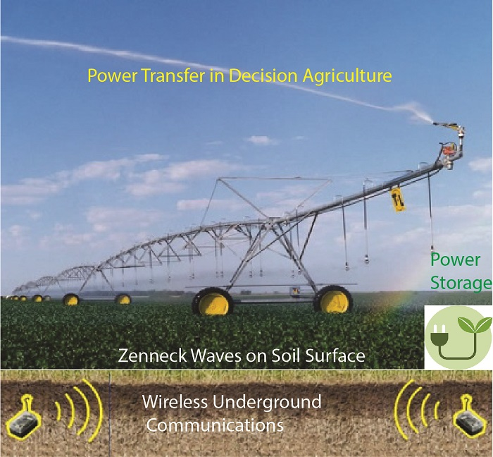
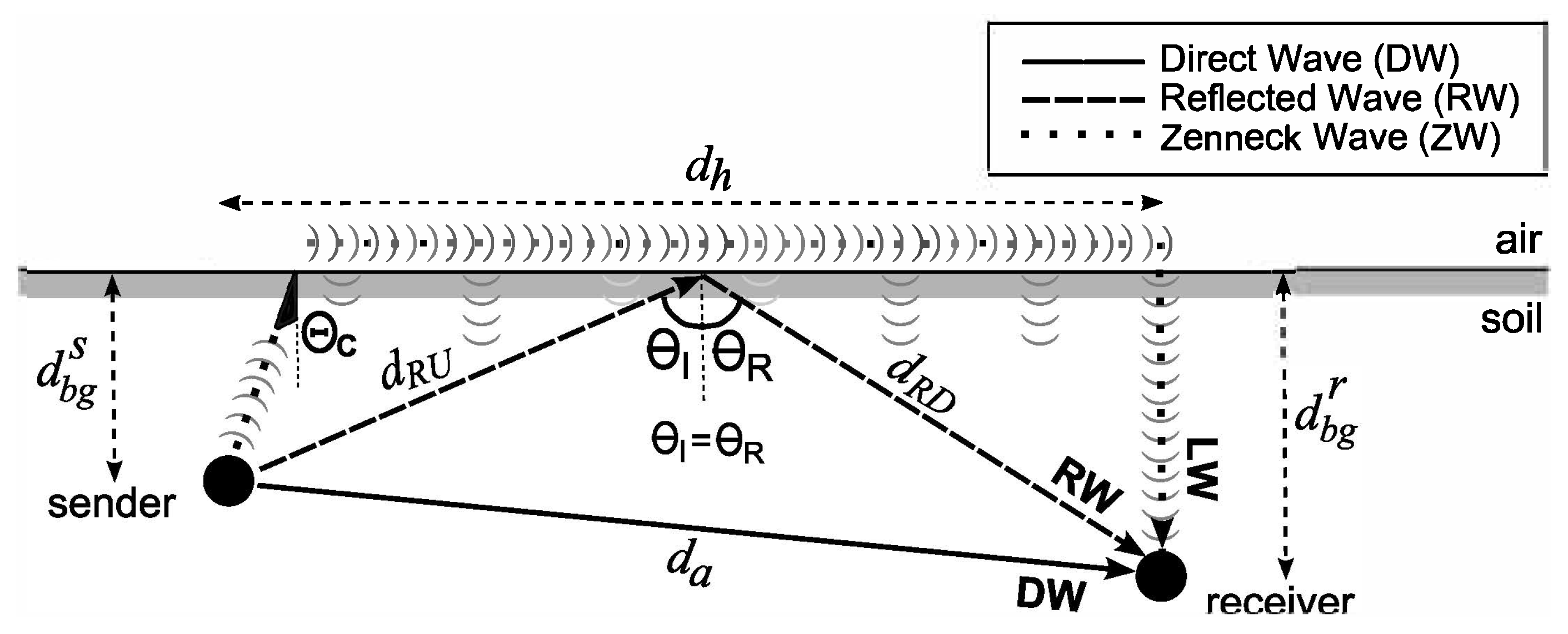
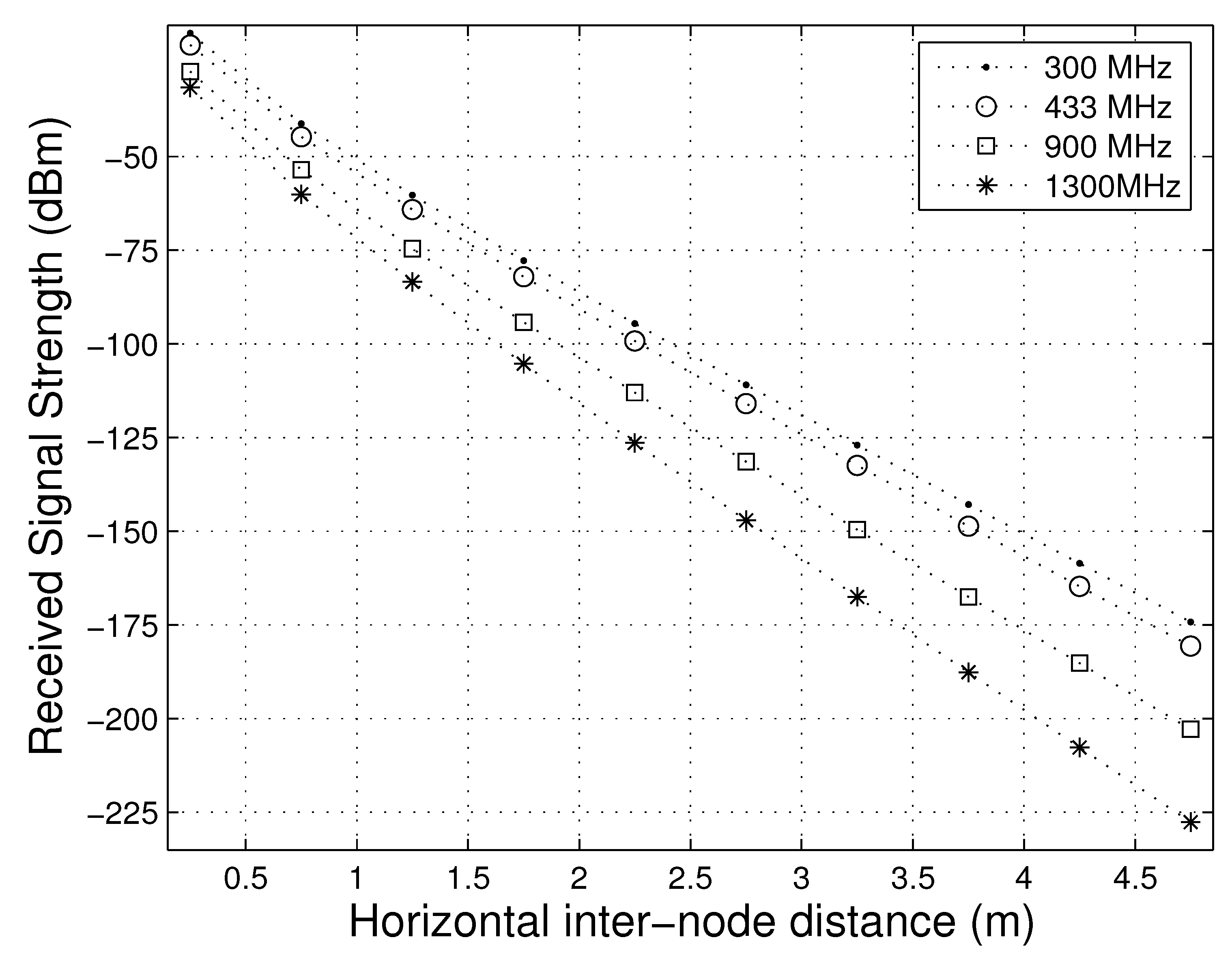
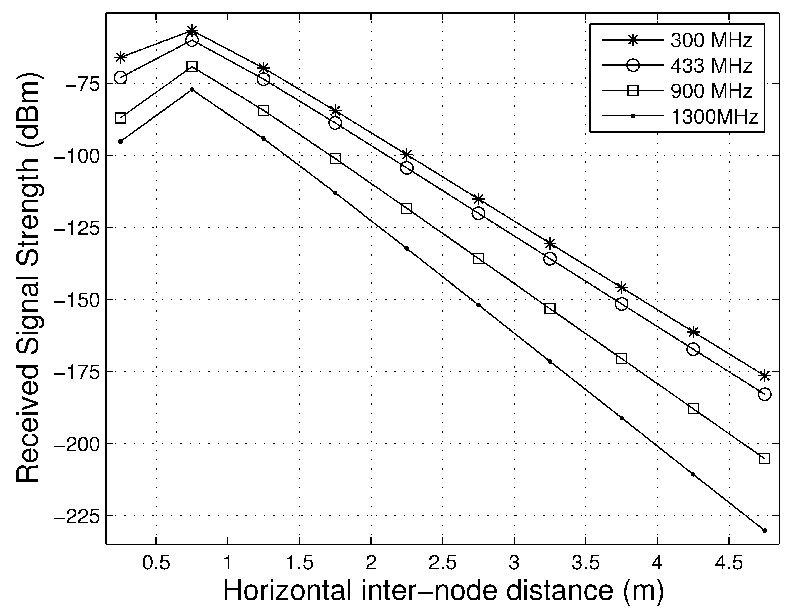
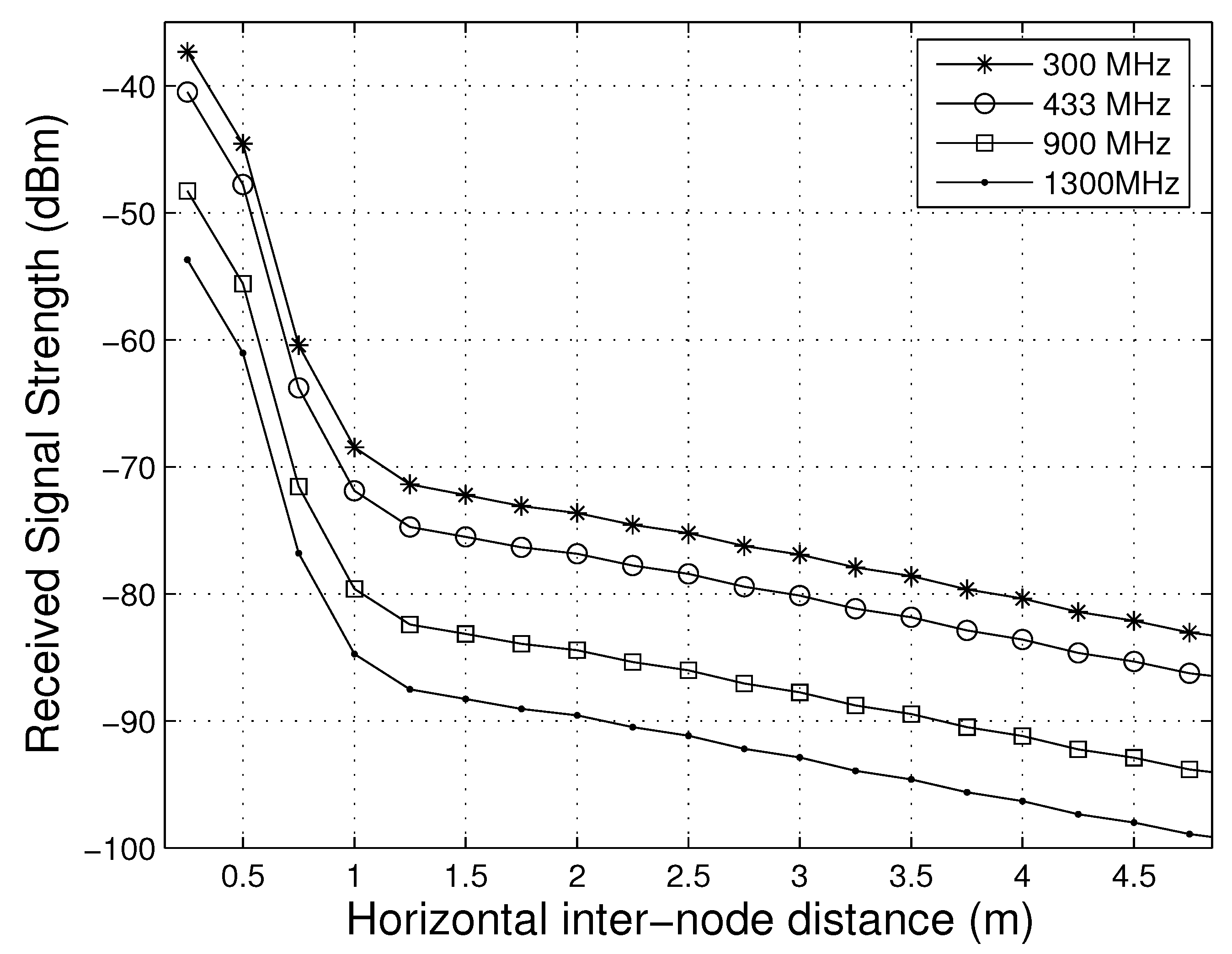
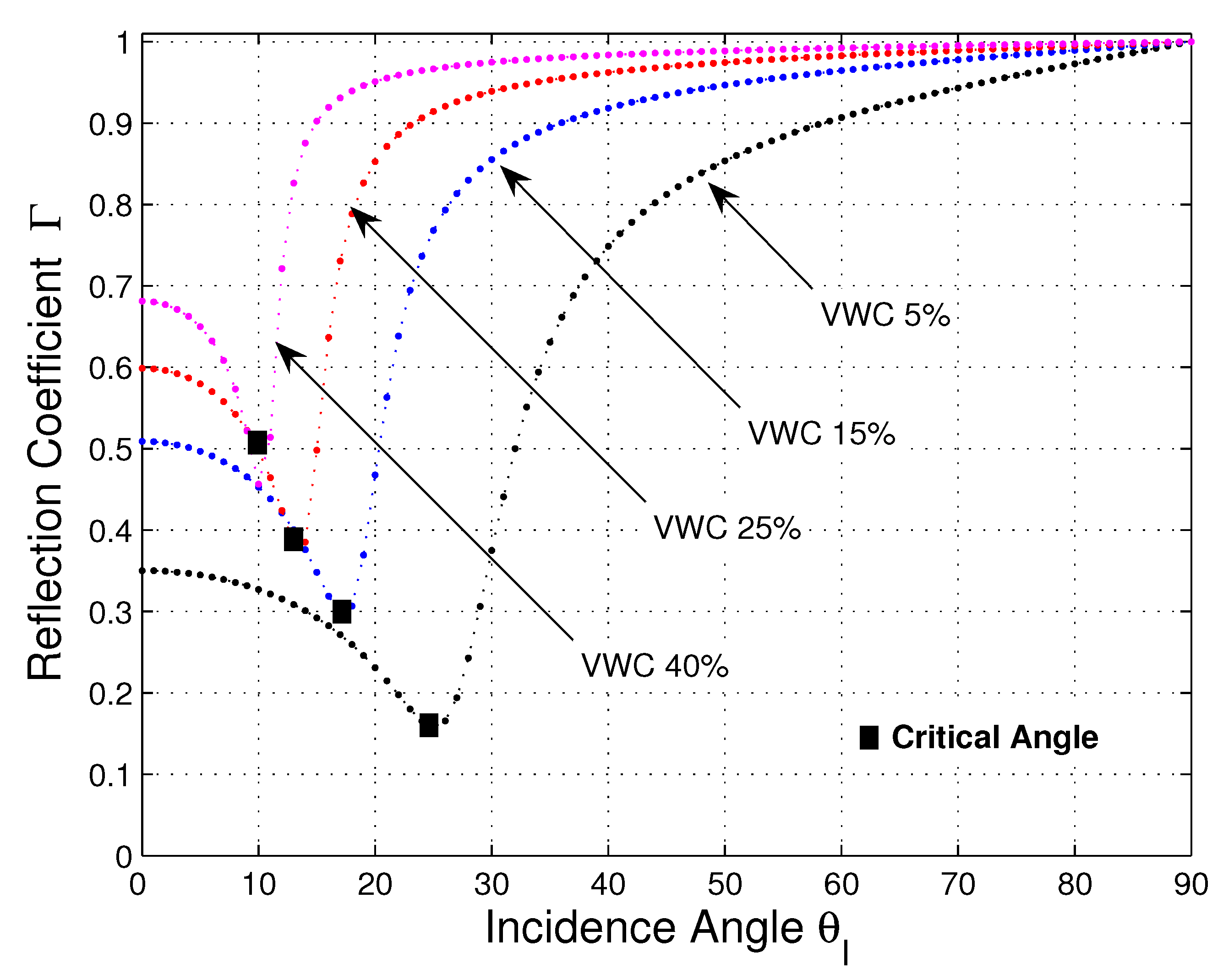
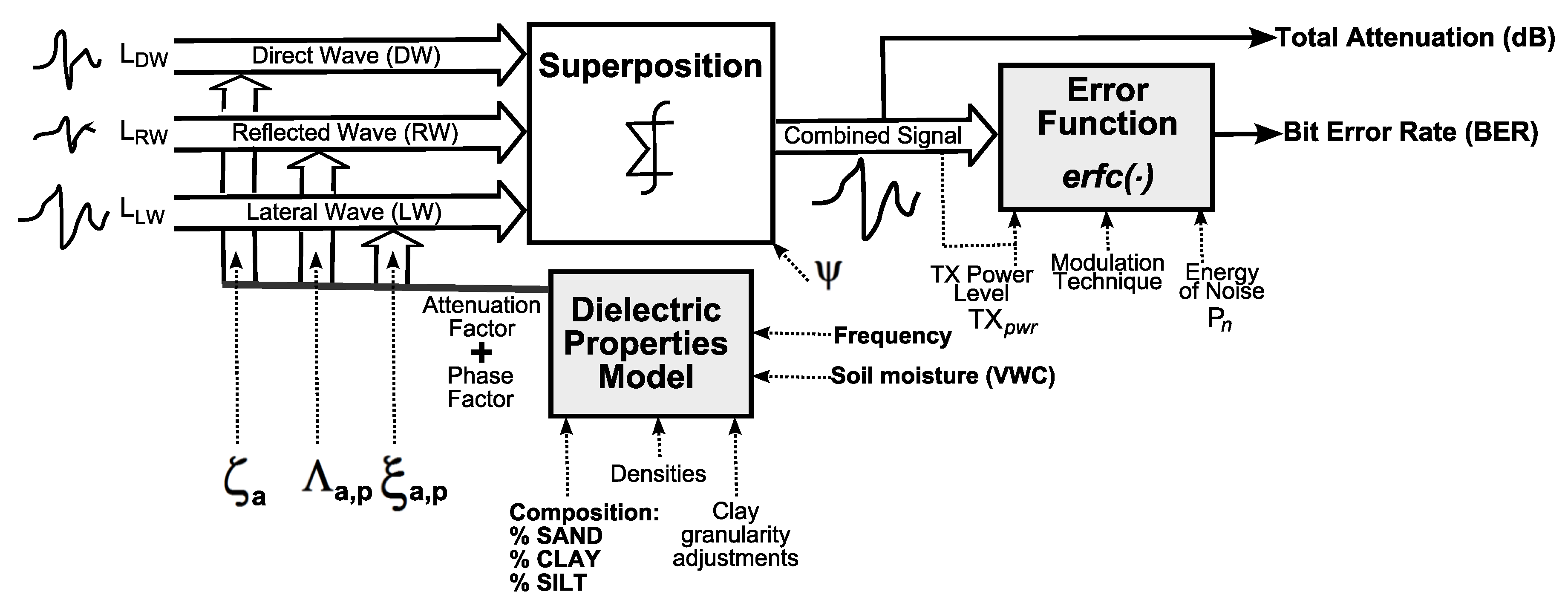
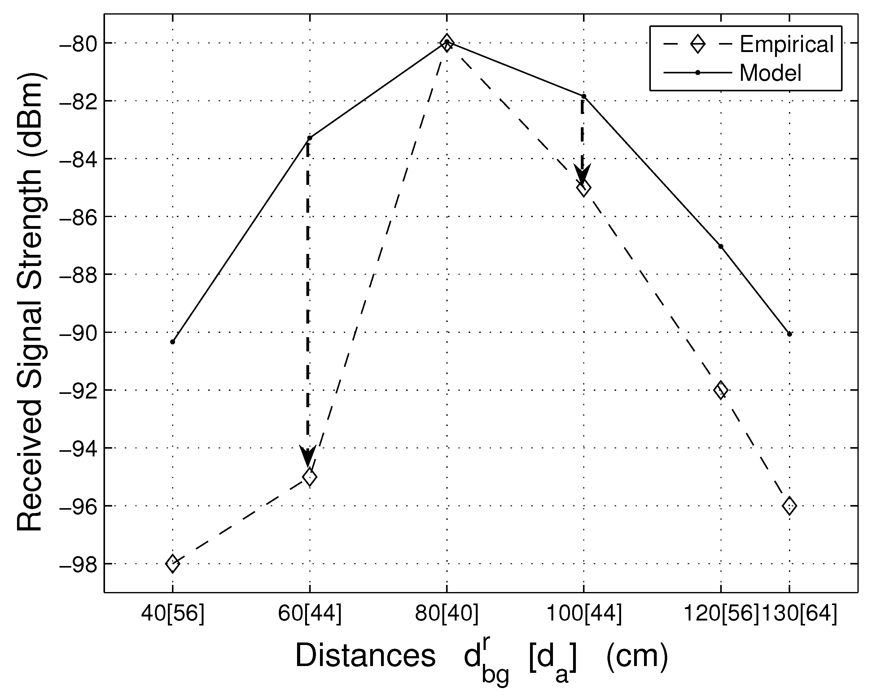
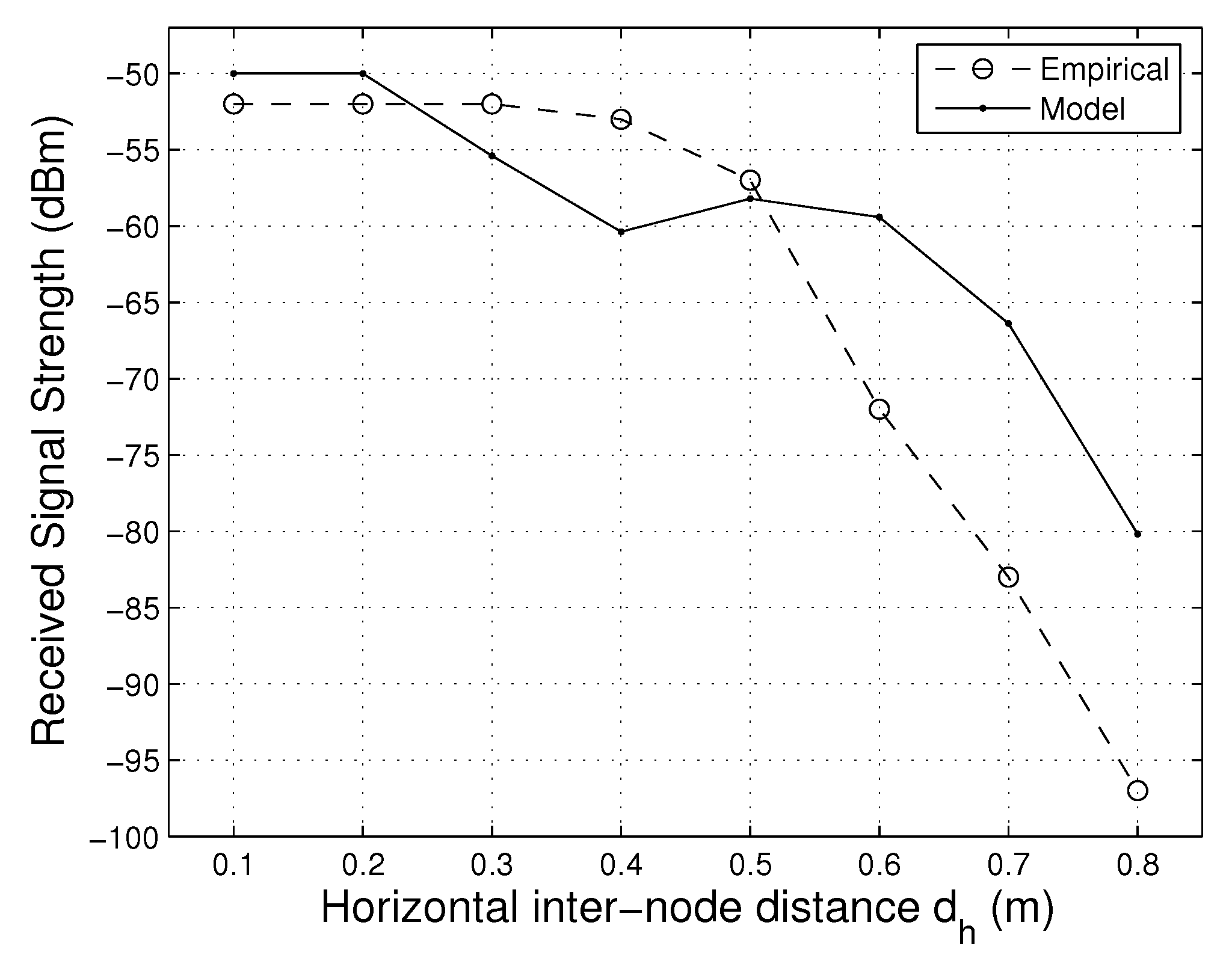
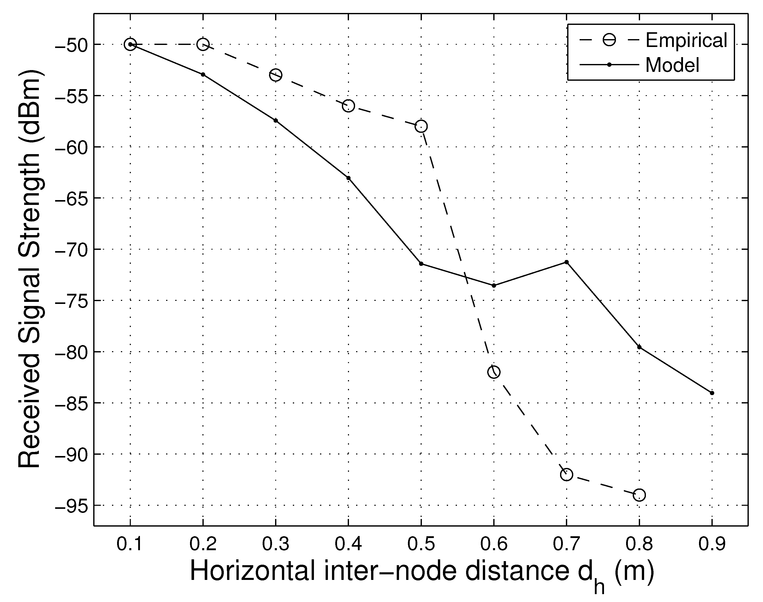
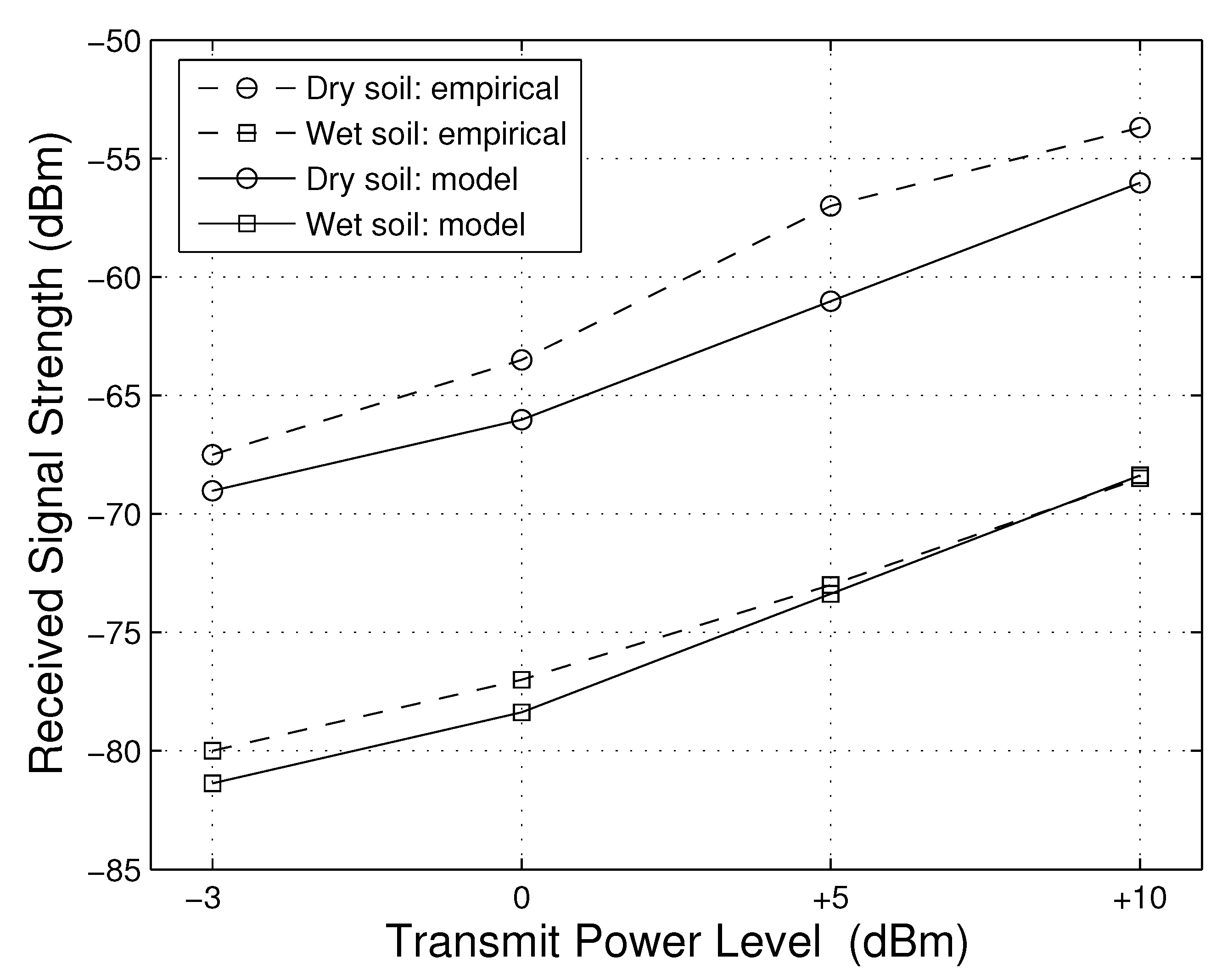
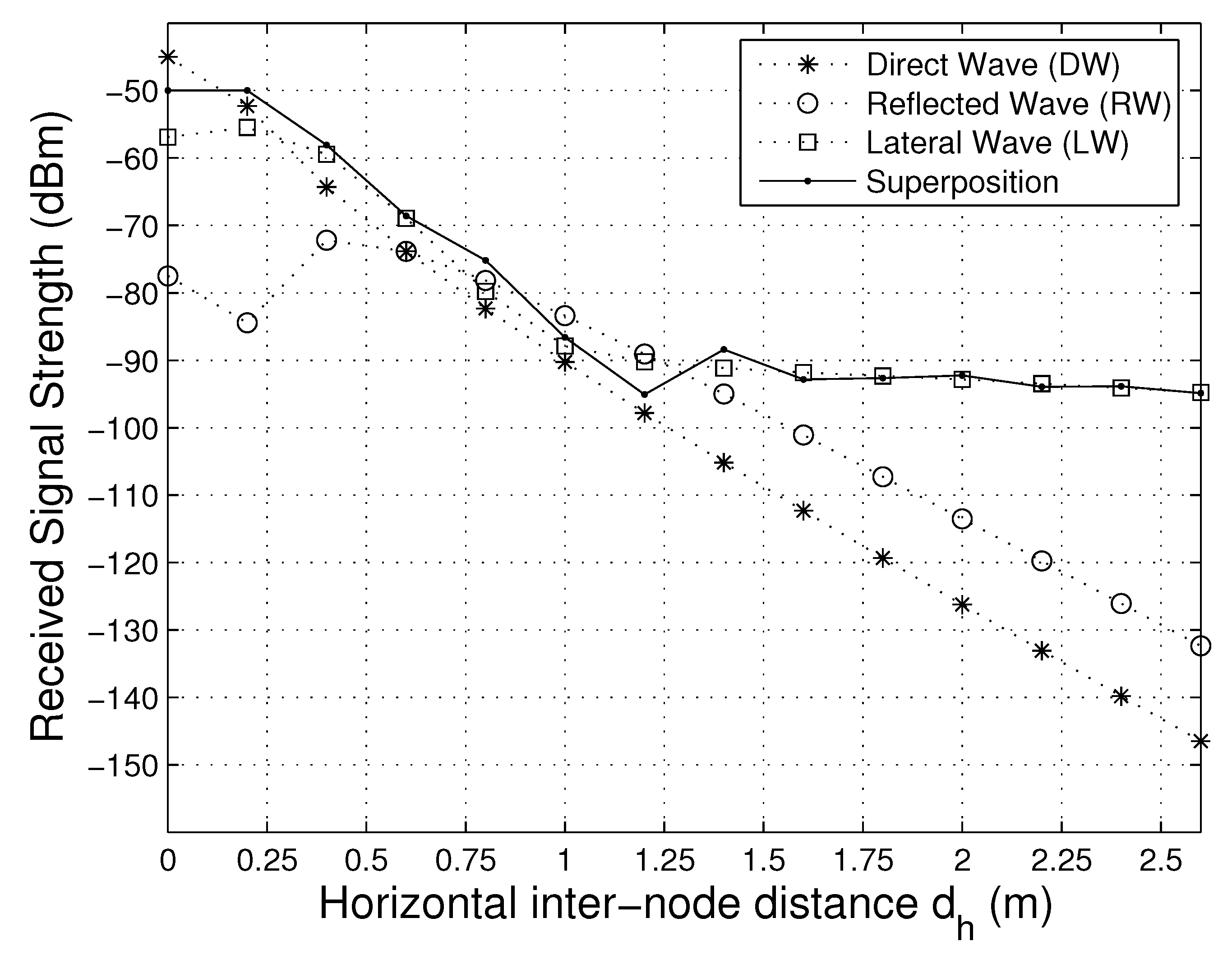
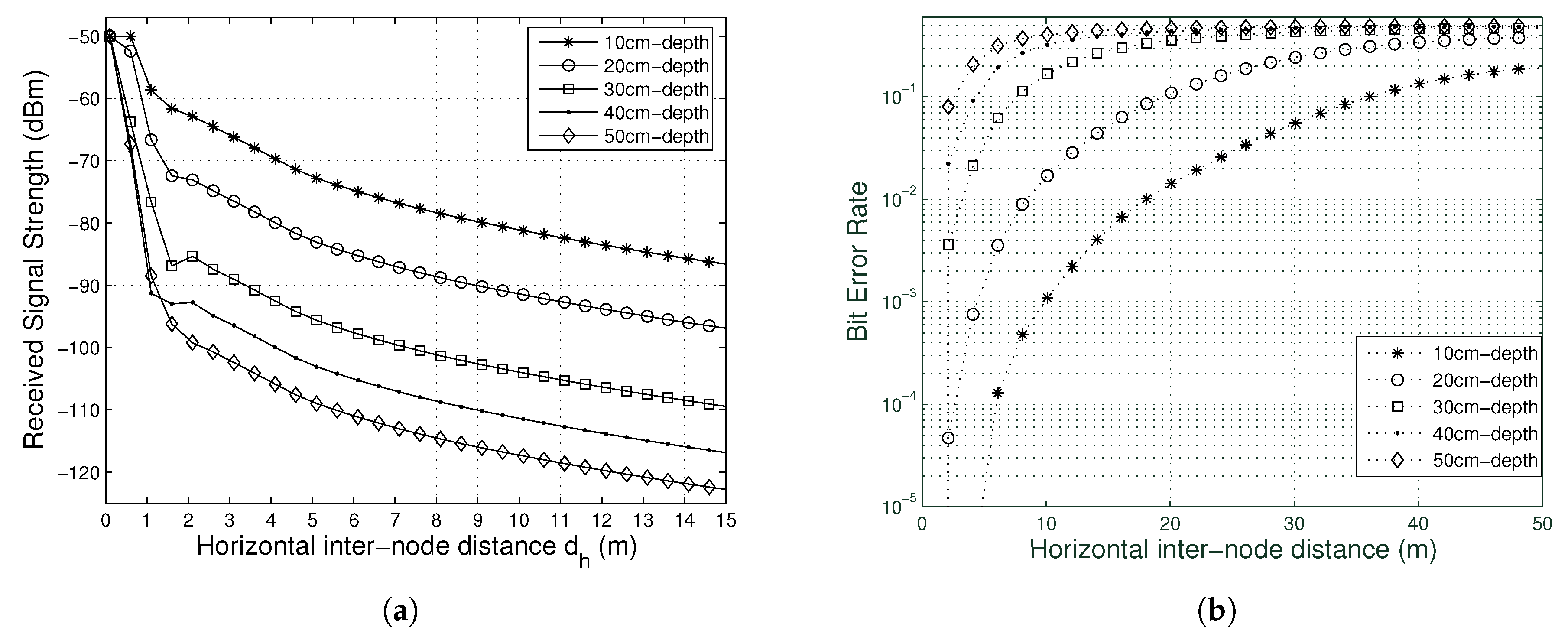
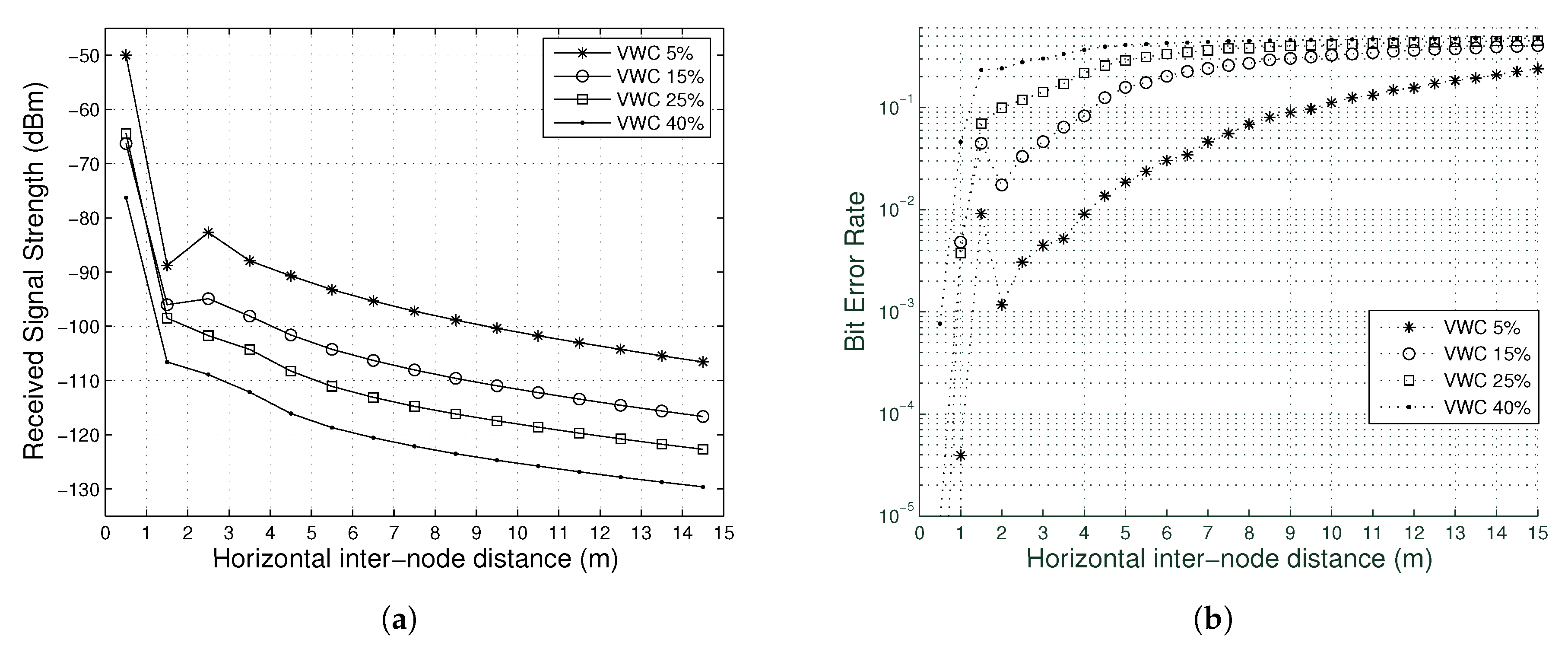
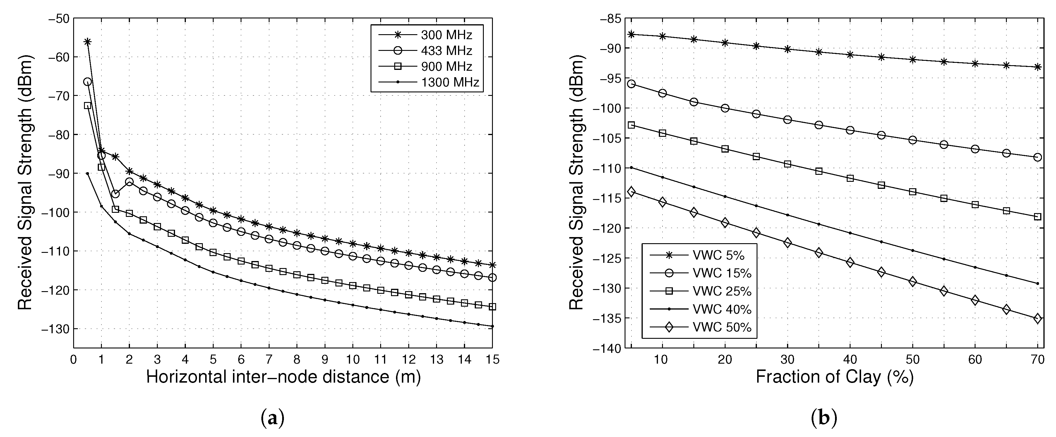
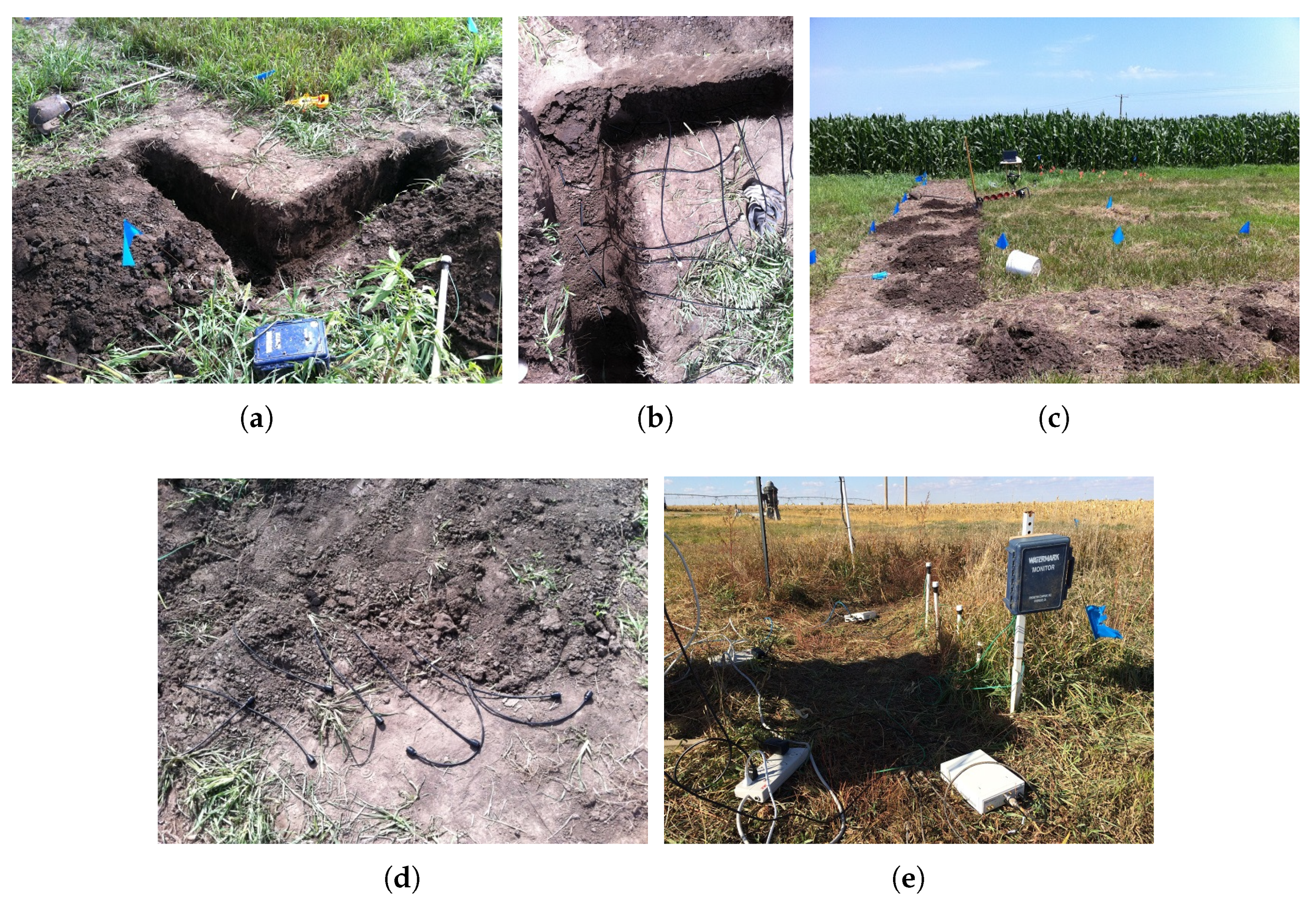
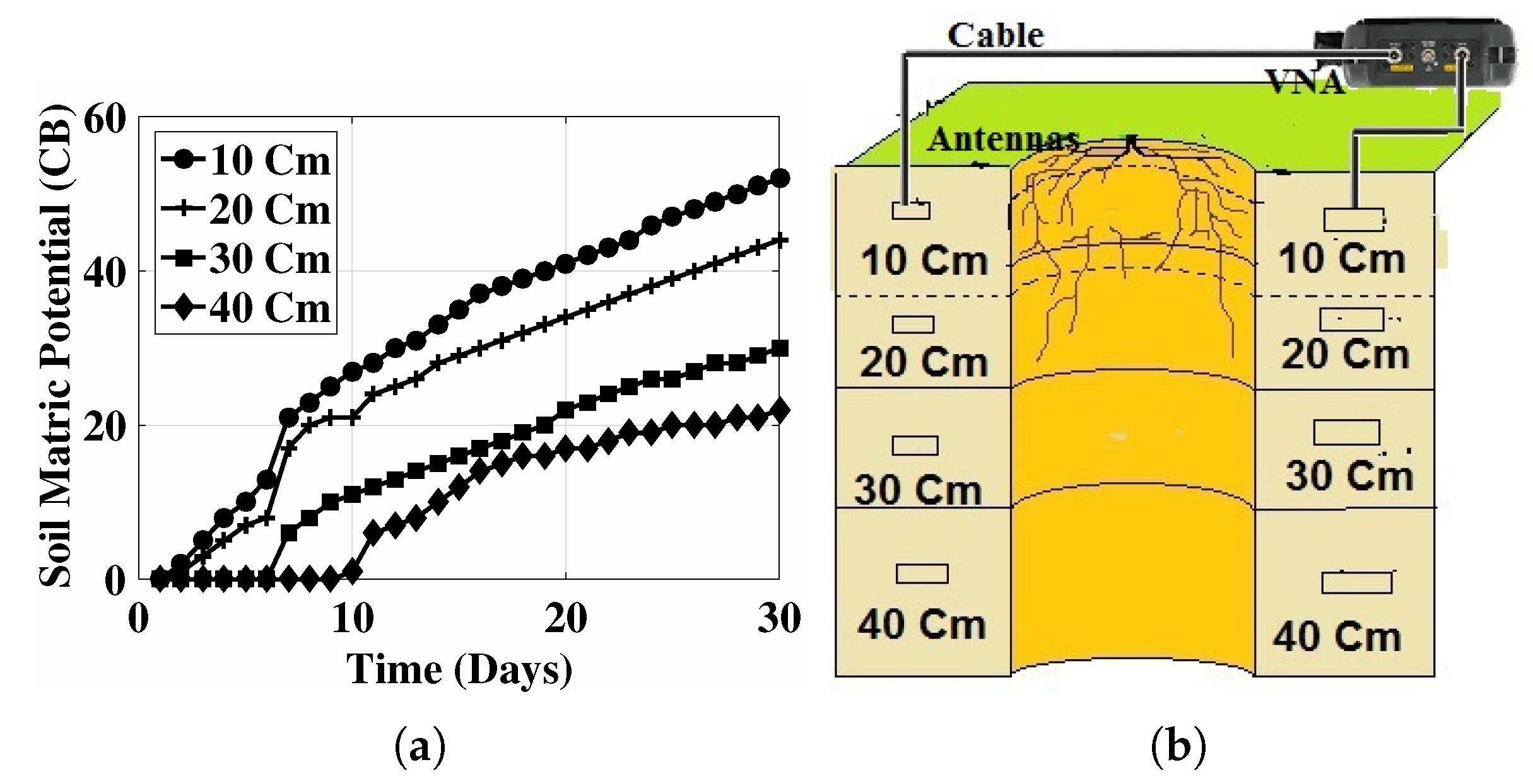
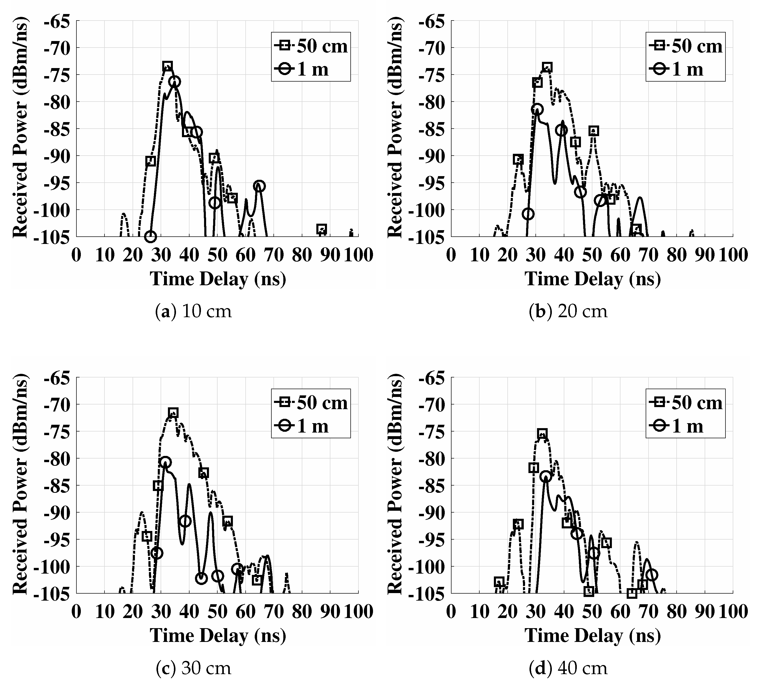
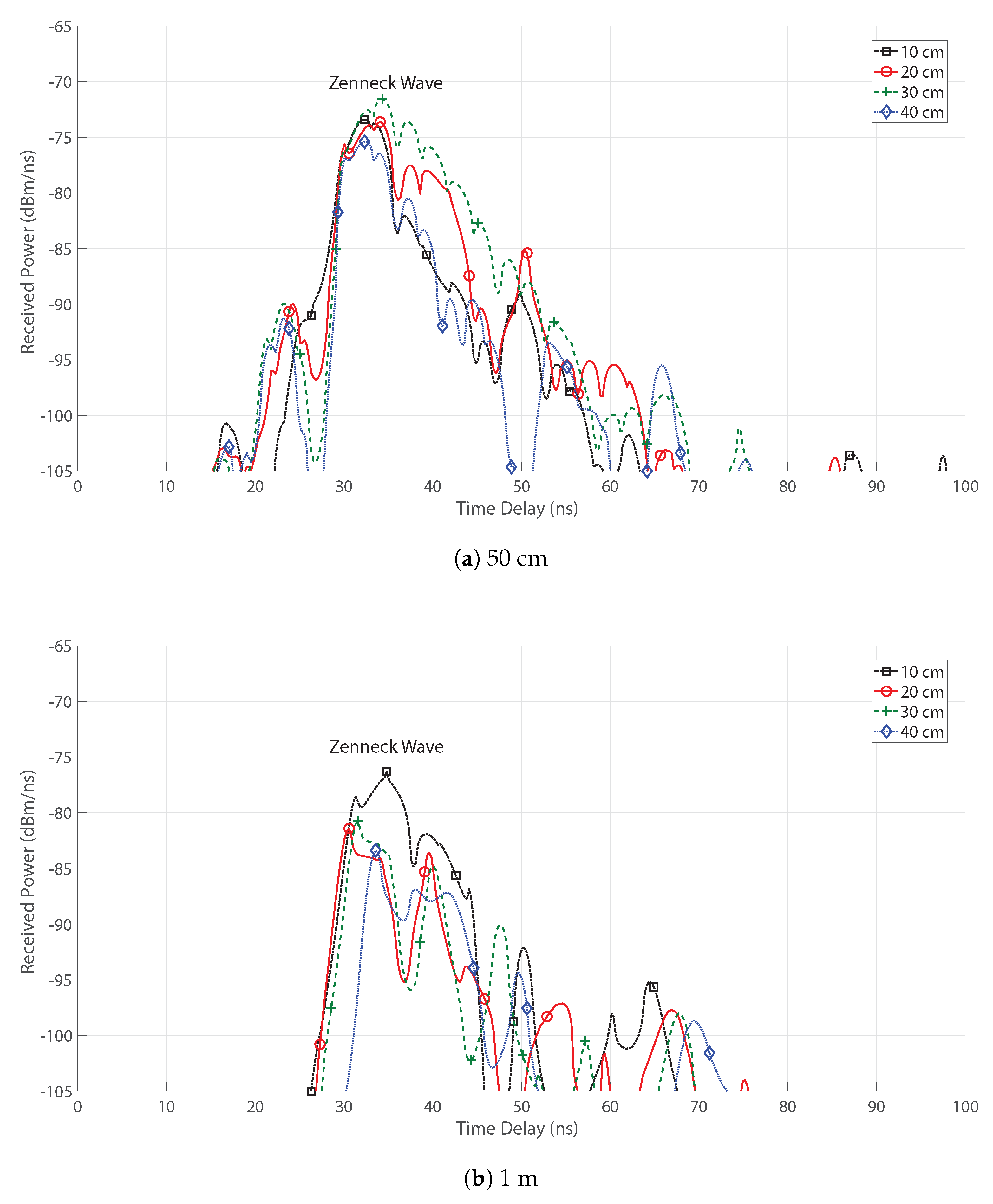
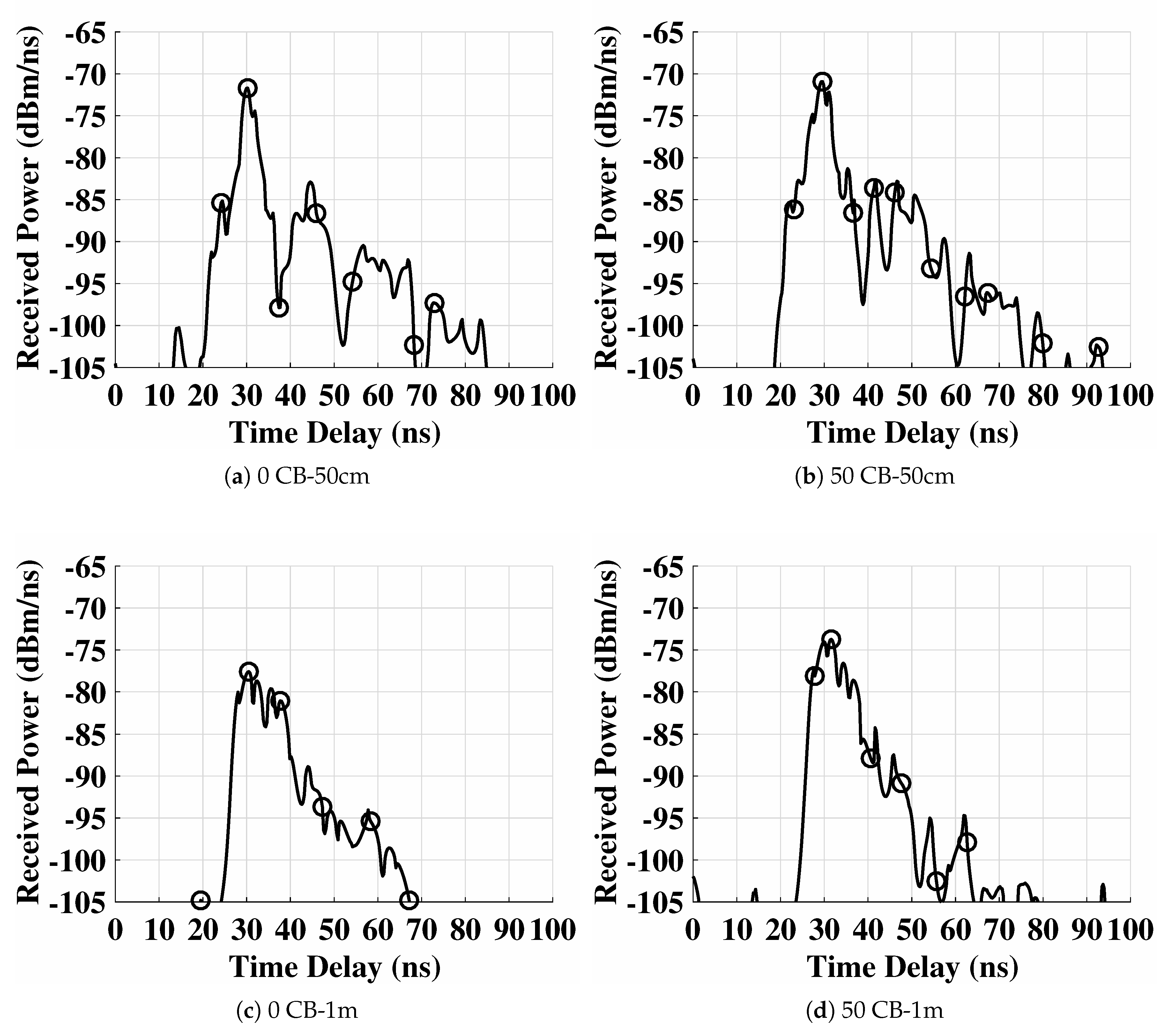
Table 1.
Parameters used in the model evaluation.
| Symbol | Description | Value |
|---|---|---|
| Bulk density | 1.33 g cm−3 | |
| Particle density | g cm−3 | |
| Particle density | g cm−3 | |
| S | Sand fraction | 35% |
| C | Clay fraction | 30% |
| - | Silt fraction | 35%, |
| Volumetric water content (VWC) | 14.6% | |
| f | Operating frequency | 433 |
| - | Antenna polarization | Parallel |
| Burial depth | 40 | |
| - | Modulation scheme | 2PSK |
| DW antenna factor | dB | |
| RW antenna factor | 17 dB | |
| LW antenna factor | 16 dB | |
| Antenna gain (sender) | 0 dB | |
| Antenna gain (receiver) | 0 dB | |
| Transmit power level | 10 dB | |
| Energy of noise | dB |
Table 2.
Particle Size Distribution and Classification of Testbed Soils.
| Textural Class | %Sand | %Silt | %Clay |
|---|---|---|---|
| Sandy Soil | 86 | 11 | 3 |
| Silt Loam | 33 | 51 | 16 |
| Silty Clay Loam | 13 | 55 | 32 |
© 2020 by the authors. Licensee MDPI, Basel, Switzerland. This article is an open access article distributed under the terms and conditions of the Creative Commons Attribution (CC BY) license (http://creativecommons.org/licenses/by/4.0/).
Share and Cite
MDPI and ACS Style
Raza, U.; Salam, A. Zenneck Waves in Decision Agriculture: An Empirical Verification and Application in EM-Based Underground Wireless Power Transfer. Smart Cities 2020, 3, 308-340. https://0-doi-org.brum.beds.ac.uk/10.3390/smartcities3020017
AMA Style
Raza U, Salam A. Zenneck Waves in Decision Agriculture: An Empirical Verification and Application in EM-Based Underground Wireless Power Transfer. Smart Cities. 2020; 3(2):308-340. https://0-doi-org.brum.beds.ac.uk/10.3390/smartcities3020017
Chicago/Turabian StyleRaza, Usman, and Abdul Salam. 2020. "Zenneck Waves in Decision Agriculture: An Empirical Verification and Application in EM-Based Underground Wireless Power Transfer" Smart Cities 3, no. 2: 308-340. https://0-doi-org.brum.beds.ac.uk/10.3390/smartcities3020017