The Controls of Iron and Oxygen on Hydroxyl Radical (•OH) Production in Soils


1
Department of Earth and Environmental Sciences, University of Michigan, Ann Arbor, MI 48109, USA
2
Department of Ecology and Evolutionary Biology, University of Michigan, Ann Arbor, MI 48109, USA
*
Author to whom correspondence should be addressed.
Soil Syst. 2019, 3(1), 1; https://0-doi-org.brum.beds.ac.uk/10.3390/soilsystems3010001
Submission received: 13 October 2018
/
Revised: 4 December 2018
/
Accepted: 19 December 2018
/
Published: 26 December 2018
(This article belongs to the Special Issue Iron and Manganese Biogeochemical Cycling in Soils)
Abstract
:Hydroxyl radical (•OH) is produced in soils from oxidation of reduced iron (Fe(II)) by dissolved oxygen (O2) and can oxidize dissolved organic carbon (DOC) to carbon dioxide (CO2). Understanding the role of •OH on CO2 production in soils requires knowing whether Fe(II) production or O2 supply to soils limits •OH production. To test the relative importance of Fe(II) production versus O2 supply, we measured changes in Fe(II) and O2 and in situ •OH production during simulated precipitation events and during common, waterlogged conditions in mesocosms from two landscape ages and the two dominant vegetation types of the Arctic. The balance of Fe(II) production and consumption controlled •OH production during precipitation events that supplied O2 to the soils. During static, waterlogged conditions, •OH production was controlled by O2 supply because Fe(II) production was higher than its consumption (oxidation) by O2. An average precipitation event (4 mm) resulted in 200 µmol •OH m−2 per day produced compared to 60 µmol •OH m−2 per day produced during waterlogged conditions. These findings suggest that the oxidation of DOC to CO2 by •OH in arctic soils, a process potentially as important as microbial respiration of DOC in arctic surface waters, will depend on the patterns and amounts of rainfall that oxygenate the soil.
1. Introduction
Oxidation of dissolved ferrous iron (Fe(II)) by oxygen (O2) produces hydroxyl radical (•OH) in soil waters [1,2,3]. •OH is an unselective oxidant capable of oxidizing dissolved organic carbon (DOC) to carbon dioxide (CO2) [3,4]. Preliminary estimates indicated that on a landscape scale the oxidation of DOC to CO2 by •OH in Alaskan Arctic soil waters is on the same order of magnitude as microbial respiration of DOC in the surface waters draining the same soils [2]. Thus, this iron-mediated abiotic oxidation of DOC may be an important component of local and regional carbon budgets in the Arctic [2,3] or at any terrestrial-aquatic interface with waterlogged soils and strong redox gradients [5,6,7]. However, the preliminary estimates of •OH’s impact on DOC oxidation in arctic soil waters were based on two untested assumptions [2]. First, it was assumed that Fe(II) in the often waterlogged, low O2 soil waters is continuously exposed to enough O2 to support the estimated daily rates of Fe(II) oxidation and •OH production. Second, it was assumed that Fe(II) production in soil waters is fast with respect to its oxidation.
It is the balance of O2 supply and Fe(II) availability that will control •OH production (Figure 1). For example, if O2 supply is slower than Fe(II) production, then O2 supply will limit •OH production. Conversely, if O2 supply is faster than Fe(II) production, then Fe(II) production will limit •OH production. O2 in soil waters is consumed by redox reactions and microbial respiration and can be supplied to soils by introduction of oxygenated rain water during precipitation events, by diffusion from the atmosphere, by lowering of the water table height and by plant aerenchyma (Figure 1) [8,9,10,11,12,13,14]. Fe(II) in soil waters is consumed by redox reactions and produced by the microbial reduction of Fe(III) [14] and mineral dissolution and desorption of Fe(II) [15,16,17]. In general, the waterlogged, low O2 soils commonly found in arctic lowlands contain high Fe(II) concentrations [2,3,18,19], suggesting more production than consumption of Fe(II).
The processes that produce Fe(II) in soil waters (e.g., predominately microbial reduction) have been shown to depend on DOC concentration and composition [14,15,17,23]. For example, quinone moieties within the aromatic fraction of DOC are thought to aid microbial reduction of Fe(III) to Fe(II) (Figure 1) [14,20,21,22]. The strong correlations between Fe(II) and DOC concentrations across arctic and boreal regions [2,3,24,25] support the role of aromatic DOC in reducing Fe(III) to produce Fe(II). Thus, the aromatic content of the DOC may be an important control on Fe(II) production.
In addition to the aromatic content of the DOC, the processes that produce Fe(II) may vary between soils of different landscape ages and vegetation types [3,26,27]. In the foothills of the Alaskan Arctic (and near our study sites), glaciations have produced young and old land surfaces (~14,000 to >250,000 years BP) [28] that have otherwise been exposed to the same climate conditions [29]. These differences in the soil age lead to varying thickness of organic soil layers, water saturation and contact with mineral soils between older and younger landscapes. On each landscape age there are two dominant vegetation types that vary by landscape position. Tussock tundra is found in the uplands and wet sedge tundra is typical of lowland areas [26,30]. Tussock tundra is characterized by a relatively lower water table resulting in wet but not consistently saturated soils with better drainage, resulting in more oxidizing conditions [26,30,31]. Tussock tundra soils are also characterized by the presence of a deeper mineral layer in the summer-time, unfrozen active layer of the soil. The lowland wet sedge areas are characterized by more waterlogged soils (higher water table), poorer drainage, more reducing conditions and higher organic matter content in the soils because mineral layer is not shallow enough to be thawed during summer [26,30,31]. These differences in landscape age, position and vegetation type lead to differences in redox conditions and soil chemistry that are expected to affect the Fe(II) production rate but this has yet to be studied.
In this study we tested whether the O2 supply rate or the Fe(II) production rate was most important for the •OH production in soils under different conditions. To integrate the effects of O2 supply and Fe(II) production on the in situ •OH production, we used intact soil mesocosms representative of natural conditions and processes in the plant-soil system through time because they integrate a relatively large surface area and typical depths of thawed soil. This approach contrasts with the prior studies on the •OH production [2,3] that aerated soil water withdrawn at one time and one location. Soil mesocosm experiments were used to determine how vegetation type and landscape age, coupled with varying O2 supply rate during precipitation events or during static waterlogged conditions, affected the •OH production and subsequent oxidation of DOC to CO2 by •OH. Our hypothesis is that the in situ •OH production in arctic soil waters is limited by Fe(II) production when O2 supply is high during precipitation events and by O2 supply when O2 supply is low during static, waterlogged conditions in the soils.
2. Materials and Methods
2.1. Tundra Soil Cores Collection
A total of 24 intact soil-plant cores (cores 28 cm diameter; length 30 ± 1 cm; Table 1, Figure S1) were collected near Toolik Lake, Alaska (68°38′00″ N, 149°36′15″) in July 2017. The soil cores were collected from two dominant landscape ages in this region (~14,000 to 100,000 years BP for Toolik, the younger landscape; and ~250,000 years BP for Imnavait, the older landscape). On each of the two landscape ages, soil cores were collected from the two dominant vegetation types (wet sedge and tussock tundra, representing ~75% of the low Arctic landscape) [32]. Wet sedge tundra is found in valleys or lowland areas near stream or lake margins where the water table is high. Wet sedge tundra is dominated by Carex chordorrhize, C. rotundata, Eriphorum aquatilis and E. angustifolium [31]. Upland from wet sedge is tussock tundra vegetation, where the water table fluctuates with precipitation but soils are often saturated due to the water holding capacity of the surface organic mat. Tussock tundra vegetation is dominated by sedges (Eriophorum vaginatum), dwarf shrubs (Betuna nana, Vaccinium vitus idaea, Ledum palustre) and mosses (Sphagnum spp., Hylocomium spp., Aulacomium spp.) [31].
2.2. Mesocosm Design
The soil cores were used for two mesocosm experiments (Figure S1). The first experiment consisted of two acclimation periods (to mimic static, waterlogged conditions) and two flushing periods (to mimic precipitation events). The first acclimation period (static) preceded the first flushing period, followed by a second acclimation period and subsequent flushing on the same cores. The second experiment used a different set of cores and consisted of only one acclimation and one flushing period. For each of the two experiments, three replicate soil cores were collected for each of the two landscape ages and each of the two vegetation types (Figure S1).
The soil cores were flushed with ~10 L of oxic deionized water (DI) immediately after core collection to establish similar conditions in each mesocosm at the start of the experiment. After the initial flush, each soil core was transferred to a 20 L plastic bucket to establish a mesocosm. Soil mesocosms were housed in large plastic coolers (46 cm × 46 cm × 84 cm). Each cooler contained three mesocosms surrounded by an ice-filled water bath to keep the temperature relatively constant and within the temperature range of soils in the summer at the field site. The water bath covered about 80% of the soil mesocosm depth and helped simulate natural conditions at and near the permafrost boundary where the soil temperatures range from 0 to 10 °C [32]. Soil temperatures were measured at two depths in the mesocosm (at the bottom of the soil and at 10 cm below the soil surface) over the acclimation and flushing periods until the end of the experiments using iButton® data loggers. The data loggers were wrapped in whirlpacks and placed in the soil when the mesocosms were established. The soil temperatures at these depths ranged from 5 to 20 °C in all of the mesocosms (measured at 60 min intervals; N = 672 and N = 336 soil temperatures made from each mesocosm of each landscape age and vegetation type age over the average 14 and 7 days of the experiments, respectively; Figure S1). The ambient air temperatures ranged from −7 °C to 23 °C (average 9 ± 0.2 SE °C) during the study period (Environmental Data Center, Toolik Field Station).
The soil mesocosms were open to the atmosphere at the top and sealed at the bottom; O2 could diffuse into the soils from the top of each mesocosm. The mesocosms were acclimated under static waterlogged conditions (i.e., no flowing water) in the water bath for four to ten days to generate the reducing conditions observed in intact soils in the field [2,3]. DI water (1–2 L) was added to the soil mesocosms during the acclimation period to account for evapotranspiration and keep the water table constant in the mesocosms.
The soil water sampled at the end of the acclimation period just before DI was added during the flushing period was assumed to represent conditions in the mesocosms during the acclimation period. After the acclimation period, each set of triplicate mesocosms for each of the two landscape ages and for each of the two vegetation types was flushed with an average of 16.8 ± 0.9 L of DI water (N = 36, average ± SE) over one to 3 h, called the “flushing period” (Figure S1). The flushing period consisted of ten individual flushes where ten soil water samples were collected every 0.2 to 2 L of DI flushed from each replicate mesocosm. The total volume of water flushed was chosen to represent precipitation events up to and in excess of the natural precipitation patterns near Toolik Field Station (Table S1). Thus, the flushing mimicked the effects of brief and rapid changes in redox conditions on concentrations of DOC and iron, their export during precipitation events and their effect on •OH production in the soil waters. During the flushing period the mesocosms were drained from the bottom and DI was added to the top to keep the water level constant. After the flushing period, each set of triplicate mesocosms was acclimated again for five to seven days under the same conditions as during the first acclimation period. After the second acclimation period each mesocosm was flushed with 12.5 ± 0.2 L (average ± SE) of DI water during the second flushing period. As in the first flushing period, ten soil water samples were collected with each volume of DI added during the second flushing period.
At the end of the experiment, subsamples were collected from each soil core from organic and mineral (if present) layers for soil moisture, bulk density, porosity and organic carbon content [33]. Soil moisture was measured as the difference in mass of a subsample of the soil before and after draining the gravimetric water and then drying the soil for two days at 105 °C in an oven. Bulk density of the soil was determined as the mass of dry soil in an entire core divided by the soil volume (dimensions of the soil contained in the core). Porosity of the soil was calculated from the volume of soil core occupied by water versus soil. The volume of soil water was determined by draining a known volume of the soil core and measuring the volume of drained (gravimetric) water. The volume of the soil was determined from the dimensions of the soil core. Organic carbon content was determined from combusting a subsample of dried soil for one day at 550 °C, assuming the mass of organic matter lost during ignition was 50 % carbon. Values are reported as an average ± SE (N = 9 for each landscape age and vegetation type, corresponding to three replicate mesocosms measured after each of the two acclimation periods for the first experiment and after the only acclimation period for the second experiment; Figure S1).
2.3. Soil Water Collection and Characterization
Soil water was collected from each mesocosm through a drain in the bottom of the bucket with 0.5 cm radius Tygon tubing flowing directly into 60 mL BOD bottles wrapped with aluminum foil until overfilled by at least one bottle volume. Temperature, pH, conductivity and dissolved oxygen were measured on unfiltered soil water in each BOD bottle immediately after soil water collection, before and then during the flushing period. pH was measured using a WTW SenTix pH 3210 meter and probe. Temperature and conductivity were measured with a WTW Cond 3210 meter and probe. Dissolved oxygen was measured (optical probe, YSI) in the soil water collected in BOD bottles and also measured on the DI water before it was flushed through the mesocosms during the simulated precipitation events to determine how much O2 was added with flushing (DI contained average 0.3 ± 0.01 SE mmol O2 L−1, N = 9).
Subsamples of soil water from each BOD bottle were filtered for analysis of dissolved organic carbon (DOC) using pre-combusted and sample-rinsed Whatman GF/F filters. DOC samples were preserved with 6 N trace-metal grade HCl and stored in the dark at 4 °C until analysis on a Shimadzu TOC-V analyzer (Coefficient of Variation ~5% on duplicate samples or standards) [34]. Subsamples of soil water from each BOD bottle were analyzed for electron donating capacity, colored and fluorescence dissolved organic matter characterization (CDOM and FDOM, respectively), total iron and Fe(II) and •OH as described below. All values for soil water chemistry are reported as the average ± standard error (SE) from the triplicate mesocosms of each landscape age and vegetation type measured after each of the two acclimation periods for the first experiment and after the only acclimation period for the second experiment (N = 9; Figure S1).
2.4. EDC and Iron Concentrations
Unfiltered triplicate soil waters were analyzed immediately for EDC, total iron and Fe(II). For the EDC measurements, we used colorimetric detection following the protocol from Trusiak et al. (2018) [2]. Total iron and Fe(II) concentrations were quantified by the ferrozine method [35] following Trusiak et al. (2018). Particulate-rich samples were centrifuged for 3 min at 32,000 rpm to separate particulates from the soil water. The settling of particulates could lead to underestimation of the amount of EDC, total iron and Fe(II) present in the soil water of the mesocosms. Absorbance for both EDC and iron was measured on a Horiba Aqualog Spectrofluorometer in 1-cm pathlength methacrylate cuvettes.
2.5. CDOM and FDOM Analysis
Soil water subsamples for CDOM and FDOM analysis were filtered using pre-combusted Whatman GF/F filters and analyzed approximately one h after the sample collection in the field using a Horiba Aqualog Spectrofluorometer [36]. CDOM and FDOM were analyzed on the soil waters in a 1-cm pathlength quartz cuvette. Fluorescence excitation-emission matrices (EEMs) of the soil water were collected over excitation and emission ranges of 240–600 nm by excitation/emission increments of 5/1.64 nm/nm, respectively. Integration times ranged from 2 to 3 s. When necessary, the soil water was diluted 2 to 6-fold with MilliQ water to less than 0.6 absorbance units (A) at 254 nm prior to the analysis [37]. EEMs were corrected for inner-filter and instrument-specific excitation and emission effects in Matlab (version 2015b). Blank EEMs were collected using MilliQ water and were subtracted from soil water EEMs to minimize the influence of water Raman peaks. Intensities of corrected soil water EEMs were converted to Raman units. Dominant peaks in the corrected soil water EEMs were identified following Cobble [38]: Peak A (λex = 250 nm; λem = 380–460 nm), Peak C (λex = 350; λem = 420–480 nm) and Peak T (λex = 275 nm; λem = 340 nm). The fluorescence index (FI) [39,40] was calculated as the ratio of emission intensity at 470 nm to emission intensity at 520 nm at an excitation wavelength of 370 nm.
2.6. •OH Concentrations
•OH was quantified using terephthalate (TPA) [41] as a probe for •OH as previously used in arctic soil waters [2,3]. •OH was quantified by adding an unfiltered soil water subsample to O2-free (stored in O2-free atmosphere in a glove box) MilliQ water containing excess TPA. •OH present was allowed to react with TPA for 24 h prior to analysis of the product of the TPA reaction with •OH (2-hydroxyterephthalic acid, hTPA) [41]. •OH concentrations were determined using standard additions of 0, 25 and 50 nM hTPA to account for matrix effects. hTPA was quantified on an Acquity Ultra High Performance H-Class LC (uPLC; Waters, Inc., Milford, MA, USA; Mississauga, Ontario, Canada) with fluorescence detection (excitation 250 nm, emission 410 nm) on an Acquity uPLC BEH C18 column (2.1 × 50 mm; 1.7 µm). The yield for hTPA formation from •OH reaction with TPA was assumed to be 35% [41].
2.7. EDC, DOC and Iron Production
EDC, DOC, total iron and Fe(II) production was calculated as the respective concentrations in the soil waters from the initial soil water collection (after the acclimation period) divided by the number of days of the acclimation period. Preliminary measurements of soil water collected before the first acclimation period showed no detectable EDC, total iron or Fe(II). Thus, to calculate EDC, total iron and Fe(II) production rates we assumed values of zero for each of these constituents at the start of the first acclimation period. To calculate the DOC production rate, we subtracted the average DOC concentration in soil water at the end of the first flushing period from the DOC concentration measured at the end of the first acclimation period. To calculate production rates after the second acclimation period, concentrations of EDC, DOC, total iron and Fe(II) at the end of the first flushing period were subtracted from the concentrations in soil water collected after the second acclimation period. For the mesocosms where the concentrations of EDC, DOC, total iron and Fe(II) were higher after the first or second individual flush than during the initial soil water collection, the average of the first two to three individual flushes was used as the initial EDC, DOC, total iron and Fe(II) concentration. The EDC, DOC, total iron and Fe(II) production was normalized to the dry mass of soil in each mesocosm. The dry mass of soil was obtained by drying a subsample a volume of soil from the mesocosm at 105 °C for 48 h and determining the loss of soil mass after drying. The difference in the mass of the soil before and after drying is the mass of water originally contained in the soil.
2.8. Dissolved O2 Consumption
Dissolved O2 consumption was calculated as the difference in the O2 concentration before the acclimation period and the O2 concentration in soil waters at the end of the acclimation period divided by the number of days of the acclimation period. This approach likely yields minimum estimates of O2 consumption because it does not account for O2 consumed during the slow diffusion of O2 into the stagnant boundary layer of the soil core. In addition, if all O2 consumption happened before the end of the acclimation period then rates of O2 consumption were faster than estimated. Dissolved O2 consumption was then normalized to the dry mass of soil in each mesocosm (Section 2.7).
2.9. •OH Production
•OH production during the flushing period was calculated as •OH concentration after the first flush volume (corresponding to up to 15 mm of precipitation) divided by the amount of O2 introduced to the mesocosms (based on the volume of DI added and O2 concentrations in DI, giving •OH per O2 added), assuming a constant yield of •OH per O2 supplied for all precipitation events up to 15 mm rain. This yield of •OH per O2 supplied was then multiplied by the amount of O2 supplied from a 4 mm per day precipitation event, the average amount of precipitation received in one day during the summer at Toolik Field Station, to give a •OH production rate per day during precipitation events. •OH production during static, waterlogged, low O2 conditions was calculated as the •OH concentration in soil water collected at the end of the acclimation period minus a starting concentration of zero (see below). •OH production during the acclimation period was divided by the number of days of the acclimation period to estimate a daily •OH production rate, which was assumed to be constant during the acclimation period. As with EDC and Fe(II) above, preliminary measurements of soil water showed no detectable •OH production prior to the start of the first acclimation period. Thus, we used a concentration of zero •OH at the beginning of the first acclimation period in order to calculate •OH production over time. For the second acclimation period, •OH concentrations at the end of the first flushing period were subtracted from the concentrations in the soil water collected after the second acclimation period and divided by the number of days of the second acclimation period.
A number of assumptions were made to estimate •OH production. First, we assumed that •OH concentrations were the values measured by the chemical probe (Section 2.6). This assumption likely results in conservative estimates of •OH production because the measured •OH during each period of the experiment is a net of •OH production and consumption given fast quenching and reaction rates of •OH with soil constituents [42]. In addition, considering that •OH was measured only from soil water flushed from the soils, •OH production from colloids or particles retained in the soils [7] was likely not detected. Thus, it is likely that more •OH was produced in the soil waters than detected during both periods of the experiment. Finally, •OH concentration in the soil water sampled from the bottom of the mesocosm was assumed to be representative of all soil water in the mesocosm (i.e., each mesocosm was assumed to be homogenous).
3. Results
3.1. Soil and Soil Water Chemistry Differed by Landscape Age and Vegetation Type
The chemical and physical properties of the soil cores differed in organic carbon content, soil moisture, porosity and bulk density between the landscape ages and vegetation types, as expected. Soil cores from the older landscape had higher soil organic carbon content, soil moisture and porosity than soil cores collected from the younger landscape (Table 1). Soil cores from wet sedge vegetation were characterized by a thick organic layer, while the cores from tussock vegetation contained both organic and mineral layers (Table 1). Wet sedge soils had lower bulk density and higher soil organic carbon, soil moisture content and porosity than tussock soils (Table 1).
All soil waters were mildly to fairly acidic, low in conductivity and dissolved oxygen and high in EDC, DOC and Fe(II) (Table 2), as expected from the previous work [2,3]. On average, Fe(II) accounted for 52 ± 3% of the EDC and 74 ± 9% of the total dissolved iron in soil waters, again consistent with previous work [2]. EDC and Fe(II) concentrations were strongly correlated (R2 = 0.9, p < 0.05, data not shown). Thus, Fe(II) concentrations are shown in Figure 2 to represent changes over time in both Fe(II) and EDC (not shown). Soil waters from the older landscape had higher EDC, DOC and Fe(II) concentrations compared to soil waters from the younger landscape. On each landscape, there were generally no significant differences in EDC, DOC, total iron and Fe(II) concentrations between the two vegetation types (t-test, Table 2).
Similar to the initial differences in soil water chemistry presented above, there were some significant differences in the DOC composition between landscape age and vegetation type (Table 3). The ratio of peak A to peak T intensity of FDOM (T/A) differed significantly by landscape age for each vegetation type. That is, when comparing soil waters from tussocks, the T/A ratio was significantly higher for soil water DOC from the younger than the older landscape soils (Table 3). Similarly, for wet sedge soil waters, the T/A ratio was significantly higher for DOC from the younger than the older landscape soils (Table 3). The DOC in soil water from older tussock soils had a significantly lower slope ratio than DOC from younger tussock soils (Table 3). The fluorescence index (FI) of DOC from older wet sedge soils was significantly higher than the FI of DOC from younger wet sedge soils (Table 3). Of the DOC from younger soils, the FI was significantly higher from tussock than from wet sedge soils (Table 3).
3.2. Change in Soil Water Chemistry During Precipitation Events
O2 concentrations decreased to low levels during the acclimation period of the experiment and increased with the amount of water flushed through the mesocosms (Figure 2). For example, following the acclimation period, the initial soil water collected from the mesocosms had low O2 (52 ± 9 µM, average ± SE, N = 36; Table 2). During the first flushing period, soil water O2 concentrations increased with increasing volume of DI water added (i.e., increased with flush volume; Figure 2) to average 230 ± 14 SE µM (N = 36; Figure 2). During the second acclimation period following the first flushing period, O2 in soil waters was consumed and returned to the low concentrations observed after the first acclimation period (Figure 2). The increase in O2 concentrations during the second flushing period was similar to that in the first flushing period (Figure 2).
During the first acclimation period, Fe(II) concentrations increased as O2 concentrations decreased in each mesocosm (shaded portions of Figure 2). Thus, Fe(II) concentrations were the highest in the soil waters just after each acclimation period (i.e., within the first or second flush; Figure 2) with an exception. For wet sedge soil waters, Fe(II) concentrations decreased during the second acclimation period and remained relatively constant during the first and second flushing periods. For tussock soil waters, Fe(II) concentrations decreased during the first and second flushing periods. Fe(II) concentrations generally decreased with increasing flush volume until concentrations were 10 µM or less, at which point they remained relatively constant or decreased less with increasing flushing (Figure 2).
Similar to Fe(II), DOC concentrations were the highest at the end of each acclimation period and generally decreased with flushing (Figure 2). An exception was wet sedge soil water, where the DOC concentrations remained relatively constant during the first and second flushing periods (Figure 2). DOC composition changed during the flushing as well. Although there was high variability in FI of the DOC between replicate mesocosms, there was a significant decrease in the FI of the DOC with flushing from each mesocosm (i.e., slope significantly less than zero; p < 0.05; data not shown). When averaged by landscape age and vegetation type, there was a significant decrease in the FI of the DOC with flushing (Figure 3). As the volume of water flushed through the soil increased, the DOC exported was thus likely more aromatic (i.e., lower FI) [39].
Changes in •OH concentration during the precipitation events and static waterlogged conditions generally followed the changes in O2, DOC and Fe(II) in the tussock soil waters (Figure 2). In the tussock soil waters, •OH was higher after the acclimation periods when O2 was low and when DOC and Fe(II) were high (Figure 2). •OH concentrations generally decreased with flushing of the tussock soil waters concurrent with increases in O2 and decreases in DOC and Fe(II). In the wet sedge soil waters, changes in •OH were less clearly coupled to changes in O2, DOC and Fe(II) (Figure 2). •OH decreased in the older landscape wet sedge soil water with flushing as O2 increased but there was less change in •OH with increasing O2 in the younger landscape wet sedge soil water. •OH increased during the second acclimation period (corresponding to the decrease in O2) in the wet sedge soil waters when DOC and Fe(II) decreased or stayed the same (Figure 2).
3.3. Consumption and Production from Waterlogged Soils
O2 consumption was higher in the older landscape wet sedge soil waters than in the younger landscape tussock soil waters (Table 4). O2 consumption was not significantly different between the first and second acclimation periods for all mesocosms, except in the older landscape wet sedge soil water where O2 consumption was lower during the second acclimation period than during the first acclimation period (Table 4).
Fe(II) and DOC were generally produced during the acclimation period and their production was positively correlated (Figure 4A,B). One exception to Fe(II) production was the net consumption of Fe(II) from wet sedge soil waters on the older landscape during the second acclimation period (Table 4, Figure 4B, negative values). During the first acclimation period, Fe(II) production rates were significantly higher from the soil waters on the older than the younger landscapes (Figure 4A). During the second acclimation period Fe(II) production rates were generally lower than or within the same range as during the first acclimation period for all soil waters, except for the tussock soil waters on the older landscape (Table 4, Figure 4B). For the older landscape tussock soil waters, Fe(II) production during the second acclimation period was significantly higher than during the first acclimation period (Figure 4B).
•OH production rates were strongly, positively correlated with Fe(II) production rates (Figure 5). Therefore, there were significant differences in •OH production between landscape ages and vegetation types. •OH production was higher from the soil waters on the older, high-iron landscapes than from the younger landscapes and higher from the soil waters in tussock than from wet sedge vegetation (Figure 5).
4. Discussion
Our results demonstrate that either Fe(II) or O2 availability could control •OH production, depending on the soil and environmental conditions that are affected by landscape age and vegetation type. For example, during precipitation events when upland soils are rapidly flushed with O2, there is high potential for •OH production due to the consumption of Fe(II) by O2. This potential may be limited by the Fe(II) production rate because Fe(II) is consumed by oxidation when soils are flushed. During static, waterlogged conditions characterized by low O2 and relatively high Fe(II) concentrations, •OH production may be limited by the O2 supply rate to oxidize Fe(II). By relating •OH production to the O2 supply and consumption and to the Fe(II) production and consumption, we assess the limits on •OH production (and its oxidation of DOC to CO2) during different redox regimes in soils occurring during precipitation events and waterlogged conditions.
4.1. The Balance of Fe(II) Production and Consumption Controls •OH Production During Precipitation Events
During precipitation events, Fe(II) exported from the soil can decrease due to dilution by rain water or consumption by oxidation or increase by production. Correcting Fe(II) export for the addition of simulated rain water (i.e., DI water containing no detectable Fe(II)) rules out a decrease in Fe(II) from dilution (Figure 6). Once corrected for dilution, Fe(II) export was relatively constant with increasing O2 added during the flushing period in all soil waters except for the older tussock (Figure 6). In older tussock soil waters, Fe(II) export corrected for dilution decreased and then was relatively constant as more O2 was supplied during the flushing period (Figure 6). Thus, these results suggest that Fe(II) production was in balance with its consumption as O2 was supplied in all soils except older tussock soils (Figure 6).
Fe(II) production with increasing O2 supplied is not expected given that Fe(II) oxidation by O2 is a sink for Fe(II) [43]. However, one process that could produce Fe(II) in the presence of O2 is the reduction of Fe(III) by reduced DOC [14,22,23,44,45,46,47]. Two lines of evidence suggest that reduction of Fe(III) by DOC could produce Fe(II) as O2 was supplied. First, the electron donating capacity (EDC) of the DOC exported from the soils likely increased during flushing. This is because the EDC of DOC increases as the DOC aromatic fraction increases [44] and the DOC flushed from soils at higher O2 was increasingly aromatic (lower FI, Figure 3). Second, the DOC export (corrected for dilution; Figure S2), was relatively constant with flushing. Together, these results suggest export of increasingly reduced DOC at higher O2 supplied (Figure 3 and Figure S2). The export of increasingly reduced DOC at higher O2 could offset the loss of reduced DOC by its oxidation by O2 [44,45,46]. Flushing aromatic DOC with a relatively higher EDC from the soils (per g DOC; Figure 3 and Figure S2) may have regenerated Fe(II) that was oxidized by O2, thereby contributing to the constant Fe(II) export with increasing O2 supply during precipitation events (Figure 6). Thus, DOC composition likely influenced the balance of Fe(II) production and consumption during precipitation events.
The balance of Fe(II) production and consumption limits •OH during precipitation events. •OH export corrected for dilution by rain water were generally relatively constant with increasing O2 supplied, which is consistent with Fe(II) production (Figure 6). For example, the relatively constant •OH export in all soil waters during a large precipitation event (≥ 3.8 mmol O2 m−2 corresponding to ≥ 15 mm of rain) [26] was likely due to the balance between Fe(II) production and consumption where there was no net change in Fe(II) concentrations (Figure 6).
4.2. O2 Supply Limits •OH Production During Waterlogged Conditions
•OH production rates quantified during the acclimation period were likely representative of •OH production rates in the soil waters during static, waterlogged conditions. During the acclimation period, the O2 supply rates to soil mesocosms were likely similar to the O2 supply rates to natural soils (e.g., O2 was supplied to the soil by diffusion or via plant roots). In addition, there was net Fe(II) production in most soil waters during the acclimation period (Figure 4) at rates comparable to field studies in other arctic soils [14] and in temperate-zone northern peatlands [12,13]. Thus, we assume that the •OH production rate measured during the acclimation period approximates a constant daily rate at which •OH is produced from the Fe(II) oxidation by O2 supplied to the soils.
Field observations suggest that the O2 supply may limit •OH production during static, waterlogged conditions. Generally during summer in the Alaskan arctic tundra, the shallow impermeable barrier of permafrost in soils results in waterlogged and reducing conditions as indicated by low dissolved O2 and high Fe(II) concentrations [2,3,48,49]. High Fe(II) concentrations suggest that Fe(II) production outpaces its consumption by O2 (and thus outpaces the O2 supply rate) during static, waterlogged conditions. However, the oxidative consumption of Fe(II) by O2 is the source of •OH [2,3,7]. Thus, if the O2 supply rate was similar to the Fe(II) production rate, then the •OH production could be higher compared to conditions when O2 supply rates are lower than Fe(II) production. The former scenario is indicated by relatively constant •OH production at relatively constant Fe(II) (the net of Fe(II) production and consumption after correction for dilution; Figure 6). If O2 supply is a limit on the •OH production in static waterlogged soils, identifying the dominant supplies of O2 to soils is crucial for understanding •OH production.
O2 supply can be much faster than Fe(II) production in any soil water, where net Fe(II) production may be up to 10 mmol Fe(II) m−2 day−1 (Table 4). First, the average O2 diffusion from the atmosphere into soil air pore spaces has been reported to be 46 ± 2.4 mmol O2 m−2 day−1 for tussock soils and 34 ± 5.5 mmol O2 m−2 day−1 for wet sedge soils [31]. Second, a 1 cm drop in the water table in an organic mat soil with a typical porosity of 60–80% would result in an increase in O2 of 60 to 80 mmol O2 m−2 for wet sedge and tussock soil waters, respectively. Changes in water table height from 1 mm up to 1 cm per day have been observed in soils underlain by permafrost [50,51,52]. Thus, a daily drop in water table height of 1 mm to 1 cm could result in a rate of O2 supply from 1–12 mmol O2 m−2 d−1. Third, O2 supply from plant roots for wetland species has been reported to be 10–130 ng O2 cm−2 root surface min−1 depending on the vegetation and the distance from the root [53]. Assuming a live fine root area index of 5 m2 root surface per m2 area of tundra [54] results in an O2 supply to the soils of 23–304 mmol O2 m−2 day−1. If Fe(II) oxidation is the only sink for O2, then faster O2 supply than Fe(II) production suggests that Fe(II) should be oxidized and not accumulate in the soil waters during static, waterlogged conditions.
There are large and fast O2 sinks other than Fe(II) oxidation that could result in limited availability of O2 in waterlogged soils. For example, respiration contributes to O2 consumption [9,31,48,55,56] and microbial respiration in arctic soil waters at our study sites has been reported to produce 2.76 ± 1.06 mol CO2 m−2 day−1 [26]. Ecosystem respiration rates in arctic and boreal soils have been reported to produce 0.2 to 0.3 mol CO2 m−2 day−1 [30,57]. In addition, O2 supplied may also be consumed during the oxidation of particulate organic matter and reduced minerals [58,59,60,61] that may not result in •OH production. Given that the respiration rates are likely much faster than the O2 supply rates, it is unlikely that all O2 supplied to the soils is used for Fe(II) oxidation and •OH production. Thus, fast O2 supply and large sinks for O2 support our results suggesting that O2 availability limits •OH production under static, waterlogged conditions.
4.3. •OH Mediated Oxidation of DOC to CO2 During Precipitation Versus Static Conditions
Results from this study show that •OH is produced from soils during precipitation events where O2 is introduced to the soil waters, as well as during static, waterlogged conditions (Figure 2). DOC is the main sink for •OH in arctic soil waters [42] and •OH oxidizes DOC to CO2 [3]. Here we compare the summer-time amount of CO2 that could be produced by •OH oxidation of DOC during precipitations events versus during static, waterlogged conditions. •OH production during a typical precipitation event was calculated using the yield of •OH per O2 supplied during flushing (Figure 6), assuming a constant yield of •OH per O2 supplied for all precipitation events up to 15 mm rain (using the average slope between the first two data points in Figure 6 for all landscape age and vegetation types). The yield of •OH per O2 supplied was then multiplied by the amount of O2 supplied from a 4 mm per day precipitation event, the average amount of precipitation received in one day during the summer at Toolik Field Station, resulting in a rate of •OH production per day during precipitation events (Table 5). The average •OH production rate from all landscape ages and vegetation types quantified during the acclimation period (Figure 5) was assumed to be the daily •OH production rate from waterlogged soils during the summer. These calculations result in rates of •OH production of 200 ± 70 µmol •OH m−2 day−1 and 60 ± 20 µmol •OH m−2 day−1 during precipitation events and during waterlogged conditions, respectively (Table 5; Appendix A and Appendix B). Assuming a yield of 1 mol CO2 per 3 mol •OH [4], the range of CO2 that could be produced from •OH oxidation of DOC is 60 ± 20 µmol CO2 m−2 day−1 and 20 ± 6 µmol CO2 m−2 day−1 during precipitation events and during waterlogged conditions, respectively (Table 5).
Assuming that the soils receive precipitation on half of the summer days and during the remaining half of the summer the soils can be characterized as static and waterlogged, then precipitation events may generate up to two to three times more •OH and CO2 production, respectively, over the summer compared to static, waterlogged conditions (Table 5; Appendix A and Appendix B). The amount of •OH and CO2 produced by precipitation events is the same order of magnitude as the prior, preliminary estimate based on the unlimited O2 supply to Fe(II)-rich soil waters [2]. Similar •OH and CO2 production from precipitation events as from conditions in soils where •OH production is not limited by O2 is consistent with the fact that O2 was not likely limiting •OH production during precipitation events (Figure 6). The amount of •OH and CO2 produced during waterlogged conditions is about five times less than the prior, preliminary estimate based on the unlimited O2 supply to Fe(II)-rich soil waters [2], consistent with the fact that O2 supply likely limits •OH production during these conditions (Figure 2). While these first comparisons of •OH and CO2 production from precipitation events versus static waterlogged conditions suggest that precipitation events may produce more •OH (and CO2), there is greater uncertainty in the production of •OH and CO2 during precipitation versus waterlogged conditions because the variation in production with the rate of O2 supply is unknown. Using the yield of •OH production per O2 supplied from the flushing period of the experiment (Figure 6) to calculate the •OH production rate during precipitation events requires an assumption that the yield of •OH per O2 supplied does not depend on the rate of O2 supplied during a precipitation event. That is, we assume the same yield of •OH per O2 supplied is independent of whether the O2 was supplied to the soils in a few h versus over the course of the day. Finally, both current (Table 5) and previous [2] landscape-scale estimates of •OH and CO2 production do not account for differences due to landscape age or vegetation type (Figure 5). Scaling the estimates of •OH and CO2 produced to the landscape requires an assessment of the landscape controls on Fe(II) and •OH production.
4.4. Landscape Controls on Fe(II) and •OH Production
Given that the magnitude of •OH production is generally controlled by the magnitude of Fe(II) production (Figure 5), it follows that •OH production is expected to be higher from tussock soils on the older landscapes that supported higher Fe(II) production (Table 4, Figure 5). Fe(II) production was highest in the older landscape tussock soil waters for two reasons. First, the mineral layer present in tussock soils was likely a source of Fe(II) from dissolution or microbial reduction (Table 1) [14,19,62]. Second, soil minerals on the older landscapes have been more extensively weathered than on the younger landscapes and thus, more carbonate has been removed from the soils on the older than on the younger landscapes [62]. Less carbonate in the older versus younger soils results in a lower pH in soil waters on the older versus younger landscapes [2,3,61] and lower pH slows the Fe(II) oxidation [43,46,62]. In addition to differences in carbonate and pH, the higher DOC concentrations in soil waters on older landscapes buffer these soils at a lower pH than soils buffered by carbonate on younger landscapes (Table 2) [63,64]. Lower pH and higher DOC in soil waters on older landscapes facilitates higher Fe(II) production by supporting mineral dissolution, desorption and microbial reduction of Fe(III) to Fe(II) [17]. Together, differences in soil chemistry between landscape ages explain why Fe(II) production was higher in tussock soil waters on older versus younger landscapes, despite the presence of a mineral layer in tussock soils on both landscapes. These results suggest that in the field, •OH production should be highest in tussock soils on older landscapes where Fe(II) production was the highest (Table 4, Figure 5).
The higher •OH production in tussock soils with higher Fe(II) production (Table 4, Figure 5) is contrary to previous studies showing the highest •OH production in wet sedge soil waters, not tussock soil waters [2,3]. In the previous studies the high •OH production from wet sedge soil waters was due to the higher Fe(II) concentrations compared to tussock soil waters, opposite of the difference in Fe(II) concentrations between wet sedge and tussock in the mesocosms (Figure 4, Table 2). Those two previous studies analyzed water withdrawn from the soil at one time, compared to the time course of analyses in intact mesocosms used in this study that integrate a larger surface area and greater depth of soil. However, while the mesocosms are much more representative of natural conditions in the bulk soil and processes through time than the methods used in prior work [2,3], they restrict the horizontal, downslope flow of water and constituents that occurs on the landscape. It is this hydrologic connectivity between upland tussock and lowland wet sedge that allows for the transfer and buildup of constituents such as Fe(II) in wet sedge soil waters [65,66,67]. Little production or even consumption of Fe(II) after the acclimation period in the wet sedge mesocosms suggests that in the field, the upland tussock soils supply dissolved constituents such as Fe(II) to the lowland wet sedge soils [2,3].
The differences in Fe(II) production and O2 supply between tussock and wet sedge soils (Table 4) suggest that •OH production will vary between these vegetation types representing differences in soil mineral layers and landscape position. The results from this study show that tussock soils have a larger reservoir of reducible iron than wet sedge soils. In addition, the upland tussock soils are better drained and experience more frequent oxidizing conditions than do wet sedge soils. Together, these characteristics of tussock soils suggest that •OH production in tussock soil waters may be dependent on the rate at which Fe(III) can be reduced to Fe(II). In contrast to tussock soil waters, wet sedge soil waters accumulate Fe(II) draining from upland tussock soils and lowland wet sedge habitats are typically poorly drained, have consistently more reducing conditions and have greater O2 consumption (Table 4) than do tussock soils. This combination of higher Fe(II) concentrations and lower O2 availability suggests that in wet sedge soil waters the supply of O2 may limit •OH production. Thus, •OH production from wet sedge soils may be greatest when precipitation events introduce O2 to a high-iron, reducing environment.
5. Conclusions
Results from this study combined with the field observations of waterlogged soils across the Arctic suggest that O2 supply is likely the predominant limit on •OH production under waterlogged conditions in arctic soils. As O2 is supplied to soils, the magnitude of •OH production that can be sustained in turn depends strongly on the Fe(II) concentration, which this study showed to depend on soil chemistry (corresponding to landscape age) and on the presence of a mineral layer (tussock soils). The capacity to sustain •OH production as O2 is supplied to soils may also depend strongly on the chemical composition and thus capacity of DOC to regenerate Fe(II) via reduction of Fe(III).
Given that the •OH (and subsequent CO2) produced by precipitation events may be about three times greater than by static, waterlogged conditions (Table 5), quantifying the importance of DOC oxidation to CO2 by •OH depends strongly on changes in the hydrologic regime in a warming Arctic. There is a high potential for DOC and Fe(II) export from reduced soils to oxic surface waters during storms or floods (this study and work [66,67,68,69]) and the frequency of heavy precipitation and inundation may increase in some regions of the arctic and subarctic in the future [70,71]. On the other hand, ice-wedge degradation occurring on the Arctic coastal plain as the permafrost thaws is predicted to alter the water balance of lowland tundra by decreasing inundation and increasing runoff [72]. In addition, most studies suggest that warming in the Arctic will result in lower water table heights [18,73,74,75] and thus increasingly oxic conditions at deeper depths in the soils than at present. This shift may also lower the depth of the oxic-anoxic interface at which Fe(II) oxidation occurs. However, •OH production from Fe(II) oxidation should continue to be important in a warming Arctic given the high abundance of iron at deeper depths in permafrost soils [63,76].
Finally, while estimates from this study indicate that CO2 produced from •OH oxidation of DOC is much less than CO2 produced by soil respiration, this process should not be discounted as unimportant in carbon budgets. For example, oxidation of DOC to CO2 at terrestrial-aquatic interfaces is a critical component of global carbon cycling e.g., [29,77,78,79]. Our results suggest that the •OH oxidation of DOC to CO2 may contribute to the high rates of element cycling and greenhouse gas production at redox gradients common at terrestrial-aquatic interfaces. These terrestrial-aquatic interfaces are currently poorly understood and poorly represented in Earth-system models. In addition, in boreal waters where DOC and dissolved iron mainly as Fe(II) have been increasing over the past 30 years [80], the availability of Fe(II) to produce •OH may be increasing. Here we show that changes in hydrology and precipitation amounts and the forms of iron and composition of DOC exported from soils, will strongly govern the CO2 production rates by this abiotic, redox-sensitive reaction involving •OH.
Supplementary Materials
The following are available online at https://0-www-mdpi-com.brum.beds.ac.uk/2571-8789/3/1/1/s1, Table S1: Summary of water additions and comparison to the natural rainfall for each set of mesocosms, Figure S1: Mesocosm experimental design, Figure S2: DOC concentration in soil waters corrected for dilution by DI water added with flushing events versus the O2 supplied during flushing.
Author Contributions
A.T., G.W.K. and R.M.C. conceived of and designed the experiments; A.T. and L.A.T. performed the experiments; A.T. and R.M.C. analyzed the data; A.T., R.M.C. and G.W.K. wrote the paper with substantial, intellectual edits from L.A.T.
Funding
Research was supported by NSF CAREER-1351745, DEB-1026843, 1637459 and 1753731, PLR-1504006 and NSF GRFP to A. Trusiak.
Acknowledgments
We thank J. Dobkowski, C. Cook, A. Deely, K. Romanowicz and researchers, technicians and support staff at the Toolik Lake Arctic LTER and Toolik Lake Field Station for assistance in the field and laboratory.
Conflicts of Interest
The authors declare no conflict of interest.
Appendix A. Calculation of •OH and CO2 Produced during a 4 mm Precipitation Event
We used the average precipitation events of 4 mm per day (Environmental Data Center, Toolik Field Station), the average amount of O2 in the DI water (17 µmol O2 per mm added), and the average •OH production yield to estimate the range in daily areal •OH production rates. Note that only one significant figure was used in the final results.
Assuming a yield of 1 mol CO2 per 3 mol •OH [4], precipitation events of 4 mm per day could result in average 60 ± 20 (SE) µmol CO2 m−2 d−1. The amount of CO2 that could be produced per unit area from •OH oxidation of DOC by precipitation events over the summer was calculated by assuming 67 rainy days per summer (number of days with > 0 mm precipitation, Environmental Data Center, Toolik Field Station):
Appendix B. Calculation of •OH and CO2 Produced during Static, Waterlogged Conditions
To estimate the average •OH and CO2 production during static, waterlogged conditions (i.e., all conditions except precipitation events) we used the average •OH production and assumed that 73 of the 140 growing days during the summer (15 May—1 October) were dry (number of days with 0 mm precipitation, Environmental Data Center, Toolik Field Station). Note that only one significant figure was used in the final results.
Assuming a yield of 1 mol CO2 per 3 mol •OH [4], waterlogged conditions during the summer would result in 1 ± 0.3 mmol CO2 m−2.
References
- Page, S.E.; Sander, M.; Arnold, W.A.; McNeill, K. Hydroxyl radical formation upon oxidation of reduced humic acids by oxygen in the dark. Environ. Sci. Technol. 2012, 46, 1590–1597. [Google Scholar] [CrossRef]
- Page, S.E.; Kling, G.W.; Sander, M.; Harrold, K.H.; Logan, J.R.; McNeill, K.; Cory, R.M. Dark formation of hydroxyl radical in arctic soil and surface waters. Environ. Sci. Technol. 2013, 47, 12860–12867. [Google Scholar] [CrossRef] [PubMed]
- Trusiak, A.; Treibergs, L.A.; Kling, G.W.; Cory, R.M. The role of iron and reactive oxygen species in the production of CO2 in arctic soil waters. Geochim. Cosmochim. Acta 2018, 224, 80–95. [Google Scholar] [CrossRef]
- Goldstone, J.V.; Pullin, M.J.; Bertilsson, S.; Voelker, B.M. Reactions of hydroxyl radical with humic substances: Bleaching, mineralization and production of bioavailable carbon substrates. Environ. Sci. Technol. 2002, 36, 364–372. [Google Scholar] [CrossRef] [PubMed]
- Hall, S.J.; Silver, W.L. Iron oxidation stimulates organic matter decomposition in humid tropical forest soils. Glob. Chang. Biol. 2013, 19, 2804–2813. [Google Scholar] [CrossRef] [PubMed]
- Minella, M.; De Laurentiis, E.; Maurino, V.; Minero, C.; Vione, D. Dark production of hydroxyl radicals by aeration of anoxic lake water. Sci. Total Environ. 2015, 527–528, 322–327. [Google Scholar] [CrossRef]
- Tong, M.; Yuan, S.; Ma, S.; Jin, M.; Liu, D.; Cheng, D.; Wang, Y. Production of Abundant Hydroxyl Radicals from Oxygenation of Subsurface Sediments. Environ. Sci. Technol. 2016, 50, 214–221. [Google Scholar] [CrossRef]
- King, J.Y.; Reeburgh, W.S.; Regli, S.K. Methane emission and transport by arctic sedges in Alaska: Results of a vegetation removal experiment. J. Geophys. Res. Atmos. 1998, 103, 29083–29092. [Google Scholar] [CrossRef] [Green Version]
- Updegraff, K.; Bridgham, S.D.; Pastor, J.; Weishampel, P.; Harth, C. Response of CO2 and CH4 emissions from peatlands to warming and water table manipulation. Ecol. Appl. 2001, 11, 311–326. [Google Scholar]
- King, J.Y.; Reeburgh, W.S.; Thieler, K.K.; Kling, G.W.; Loya, W.M.; Johnson, L.C.; Nadelhoffer, K.J. Pulse-labeling studies of carbon cycling in Arctic tundra ecosystems: The contribution of photosynthates to methane emission. Glob. Biogeochem. Cycles 2002, 16, 1–8. [Google Scholar] [CrossRef]
- Zona, D.; Oechel, W.C.; Kochendorfer, J.; Paw, U.K.T.; Salyuk, A.N.; Olivas, P.C.; Lipson, D.A. Methane fluxes during the initiation of a large-scale water table manipulation experiment in the Alaskan Arctic tundra. Glob. Biogeochem. Cycles 2009, 23, 1–11. [Google Scholar] [CrossRef]
- Knorr, K.H.; Glaser, B.; Blodau, C. Fluxes and 13C isotopic composition of dissolved carbon and pathways of methanogenesis in a fen soil exposed to experimental drought. Biogeosciences 2008, 5, 1457–1473. [Google Scholar] [CrossRef]
- Knorr, K.H.; Oosterwoud, M.R.; Blodau, C. Experimental drought alters rates of soil respiration and methanogenesis but not carbon exchange in soil of a temperate fen. Soil Biol. Biochem. 2008, 40, 1781–1791. [Google Scholar] [CrossRef]
- Lipson, D.A.; Jha, M.; Raab, T.K.; Oechel, W.C. Reduction of iron (III) and humic substances plays a major role in anaerobic respiration in an Arctic peat soil. J. Geophys. Res. Biogeosci. 2010, 115, 1–13. [Google Scholar] [CrossRef]
- Stumm, W.; Sulzberger, B. The cycling of iron in natural environments: Considerations based on laboratory studies of heterogeneous redox processes. Geochim. Cosmochim. Acta 1992, 56, 3233–3257. [Google Scholar] [CrossRef]
- Luther, G.W.; Kostka, J.E.; Church, T.M.; Sulzberger, B.; Stumm, W. Seasonal iron cycling in the salt-marsh sedimentary environment: The importance of ligand complexes with Fe(II) and Fe(III) in the dissolution of Fe(III) minerals and pyrite, respectively. Mar. Chem. 1992, 40, 81–103. [Google Scholar] [CrossRef]
- Weber, K.A.; Achenbach, L.A.; Coates, J.D. Microorganisms pumping iron: Anaerobic microbial iron oxidation and reduction. Nat. Rev. Microbiol. 2006, 4, 752–764. [Google Scholar] [CrossRef]
- Lipson, D.A.; Zona, D.; Raab, T.K.; Bozzolo, F.; Mauritz, M.; Oechel, W.C. Water-table height and microtopography control biogeochemical cycling in an Arctic coastal tundra ecosystem. Biogeosciences 2012, 9, 577–591. [Google Scholar] [CrossRef] [Green Version]
- Herndon, E.M.; Yang, Z.; Bargar, J.; Janot, N.; Regier, T.Z.; Graham, D.E.; Liang, L. Geochemical drivers of organic matter decomposition in arctic tundra soils. Biogeochemistry 2015, 126, 397–414. [Google Scholar] [CrossRef]
- Roden, E.E.; Wetzel, R.G. Organic carbon oxidation and suppression of methane production by microbial Fe(III) oxide reduction in vegetated and unvegetated freshwater wetland sediments. Limnol. Oceanogr. 1996, 41, 1733–1748. [Google Scholar] [CrossRef] [Green Version]
- Lovley, D.R.; Phillips, E.J.P. Novel Mode of Microbial Energy Metabolism: Organic Carbon Oxidation Coupled to Dissimilatory Reduction of Iron or Manganese. Appl. Environ. Microbiol. 1988, 54, 1472–1480. [Google Scholar] [PubMed]
- Roden, E.E.; Kappler, A.; Bauer, I.; Jiang, J.; Paul, A.; Stoesser, R. Extracellular electron transfer through microbial reduction of solid-phase humic substances. Nat. Geosci. 2010, 3, 417–421. [Google Scholar] [CrossRef]
- Lovley, D.R.; Phillips, E.J.P. Organic-Matter Mineralization with Reduction of Ferric Iron in Anaerobic Sediments. Appl. Environ. Microbiol. 1986, 51, 683–689. [Google Scholar] [PubMed]
- Knorr, K.H. DOC-dynamics in a small headwater catchment as driven by redox fluctuations and hydrological flow paths—Are DOC exports mediated by iron reduction/oxidation cycles? Biogeosciences 2013, 10, 891–904. [Google Scholar] [CrossRef]
- Weyhenmeyer, G.A.; Prairie, Y.T.; Tranvik, L.J. Browning of boreal freshwaters coupled to carbon-iron interactions along the aquatic continuum. PLoS ONE 2014, 9, e88104. [Google Scholar] [CrossRef] [PubMed]
- Judd, K.E.; Kling, G.W. Production and export of dissolved C in arctic tundra mesocosms: The roles of vegetation and water flow. Biogeochemistry 2002, 60, 213–234. [Google Scholar] [CrossRef]
- Ward, C.P.; Cory, R.M. Chemical composition of dissolved organic matter draining permafrost soils. Geochim. Cosmochim. Acta 2015, 167, 63–79. [Google Scholar] [CrossRef] [Green Version]
- Hamilton, T.D. Glacial Geology of the Toolik Lake and Upper Kuparuk River Regions; Biological Papers of the University of Alaska; University of Alaska: Fairbanks, Alaska, 2003; pp. 1–24. [Google Scholar]
- Kling, G.W.; Kipphut, G.W.; Miller, M.C. Arctic lakes and streams as gas conduits to the atmosphere: Implications for tundra carbon budgets. Science 1991, 251, 298–301. [Google Scholar] [CrossRef]
- Johnson, L.C.; Shaver, G.R.; Giblin, A.E.; Nadelhoffer, K.J.; Rastetter, E.R.; Laundre, J.A.; Murray, G.L. Effects of drainage and temperature on carbon balance of tussock tundra microcosms. Oecologia 1996, 108, 737–748. [Google Scholar] [CrossRef]
- Gebauer, R.L.E.; Tenhunen, J.D.; Reynolds, J.F. Soil aeration in relation to soil physical properties, nitrogen availability and root characteristics within an arctic watershed. Plant Soil 1996, 178, 37–48. [Google Scholar] [CrossRef]
- Hobbie, J.E.; Kling, G.W. (Eds.) A Changing Arctic: Ecological Consequences for Tundra, Streams and Lakes; Oxford University Press: Oxford, UK, 2014; p. 331. [Google Scholar]
- Robertson, G.P.; Bledsoe, C.S.; Coleman, D.C.; Sollins, P. (Eds.) Standard Soil Methods for Long-Term Ecological Research; Oxford University Press: New York, NY, USA, 1999. [Google Scholar]
- Kling, G.W.; Kipphut, G.W.; Miller, M.M.; O’Brien, W.J. Integration of lakes and streams in a landscape perspective: The importance of material processing on spatial patterns and temporal coherence. Freshwater Biol. 2000, 43, 477–497. [Google Scholar] [CrossRef]
- Stookey, L.L. Ferrozine—A new spectrophotometric reagent for iron. Anal. Chem. 1970, 42, 779–781. [Google Scholar] [CrossRef]
- Cory, R.M.; Miller, M.P.; McKnight, D.M.; Guerard, J.J.; Miller, P.L. Effect of instrument-specific response on the analysis of fulvic acid fluorescence spectra. Limnol. Oceanogr. Methods 2010, 8, 67–78. [Google Scholar] [Green Version]
- Miller, W.L. Recent Advances in the Photochemistry of Natural Dissolved Organic Matter. In Aquatic and Surface Photochemistry; CRC Press: Boca Raton, FL, USA, 2010; pp. 111–128. [Google Scholar]
- Coble, P.G. Characterization of marine and terrestrial DOM in seawater using excitation-emission matrix spectroscopy. Mar. Chem. 1996, 51, 325–346. [Google Scholar] [CrossRef]
- McKnight, D.M.; Boyer, E.W.; Westerhoff, P.K.; Doran, P.T.; Kulbe, T.; Andersen, D.T. Spectrofluorometric characterization of dissolved organic matter for indication of precursor organic material and aromaticity. Limnol. Oceanogr. 2001, 46, 38–48. [Google Scholar] [CrossRef] [Green Version]
- Cory, R.M.; Mcknight, D.M.; Chin, Y.; Miller, P.; Jaros, C.L. Chemical characteristics of fulvic acids from Arctic surface waters: Microbial contributions and photochemical transformations. J. Geophys. Res. Biogeosci. 2007, 112, 1–14. [Google Scholar] [CrossRef]
- Page, S.E.; Arnold, W.A.; McNeill, K. Terephthalate as a probe for photochemically generated hydroxyl radical. J. Environ. Monit. JEM 2010, 12, 1658–1665. [Google Scholar] [CrossRef]
- Page, S.E.; Logan, J.R.; Cory, R.M.; McNeill, K. Evidence for dissolved organic matter as the primary source and sink of photochemically produced hydroxyl radical in arctic surface waters. Environ. Sci. Process. Impacts 2014, 16, 807–822. [Google Scholar] [CrossRef]
- Stumm, W.; Lee, F.G. Oxygenation of ferrous iron. Ind. Eng. Chem. 1961, 53, 143–146. [Google Scholar] [CrossRef]
- Aeschbacher, M.; Graf, C.; Scwarzenbach, R.P.; Sander, M. Antioxidant properties of humic substances. Environ. Sci. Technol. 2012, 46, 4916–4925. [Google Scholar] [CrossRef]
- Klüpfel, L.; Piepenbrock, A.; Kappler, A.; Sander, M. Humic substances as fully regenerable electron acceptors in recurrently anoxic environments. Nat. Geosci. 2014, 7, 195–200. [Google Scholar] [CrossRef]
- Heitmann, T.; Goldhammer, T.; Beer, J.; Blodau, C. Electron transfer of dissolved organic matter and its potential significance for anaerobic respiration in a northern bog. Glob. Chang. Biol. 2007, 13, 1771–1785. [Google Scholar] [CrossRef]
- Voelker, B.M.; Sulzberger, B. Effects of fulvic acid on Fe(II) oxidation by hydrogen peroxide. Environ. Sci. Technol. 1996, 30, 1106–1114. [Google Scholar] [CrossRef]
- Yarie, J.; Van Cleve, K.; Dyrness, C.T.; Oliver, L.; Levison, J.; Erickson, R. Soil-solution chemistry in relation to forest succession on the Tanana River floodplain, interior Alaska. Can. J. For. Res. 1993, 23, 928–940. [Google Scholar] [CrossRef]
- Petrone, K.C.; Jones, J.B.; Hinzman, L.D.; Boone, R.D. Seasonal export of carbon, nitrogen and major solutes from Alaskan catchments with discontinuous permafrost. J. Geophys. Res. Biogeosci. 2006, 111, 1–13. [Google Scholar] [CrossRef]
- Vourlitis, G.L.; Oechel, W.C. Landscape-Scale CO2, H2O Vapour and Energy Flux of Moist-Wet Coastal Tundra Ecosystems over Two Growing Seasons A. Br. Ecol. Soc. 1997, 85, 575–590. [Google Scholar]
- Liljedahl, A.K.; Hinzman, L.D.; Harazono, Y.; Zona, D.; Tweedie, C.E.; Hollister, R.D.; Engstrom, R. Nonlinear controls on evapotranspiration in arctic coastal wetlands. Biogeosciences 2011, 8, 3375–3389. [Google Scholar] [CrossRef] [Green Version]
- Liljedahl, A.K.; Boike, J.; Daanen, R.P.; Fedorov, A.N.; Frost, G.V.; Grosse, G.; Hinzmanm, L.D.; Iilma, Y.; Jorgenson, J.C.; Matveyeva, N.; et al. Pan-Arctic ice-wedge degradation in warming permafrost and its influence on tundra hydrology. Nat. Geosci. 2016, 9, 312. [Google Scholar] [CrossRef]
- Armstrong, W. Oxygen Diffusion from the Roots of Some British Bog Plants. Nature 1964, 204, 801–802. [Google Scholar] [CrossRef]
- Soukup, A.; Armstrong, W.; Schreiber, L.; Franke, R.; Votrubová, O. Apoplastic barriers to radial oxygen loss and solute penetration: A chemical and functional comparison of the exodermis of two wetland species, Phragmites australis and Glyceria maxima. New Phytol. 2007, 173, 264–278. [Google Scholar] [CrossRef]
- Jackson, R.B.; Mooney, H.A.; Schulze, E.-D. A global budget for fine root biomass, surface area and nutrient contents. Proc. Natl. Acad. Sci. USA 1997, 94, 7362–7366. [Google Scholar] [CrossRef] [PubMed]
- Stuart, L.; Miller, P.C. Nordic Society Oikos Soil Oxygen Flux Measured Polarographically in an Alaskan Tussock Tundra A. Proc. Natl. Acad. Sci. USA 1981, 5, 139–144. [Google Scholar]
- Huemmrich, K.F.; Kinoshita, G.; Gamon, J.A.; Houston, S.; Kwon, H.; Oechel, W.C. Tundra carbon balance under varying temperature and moisture regimes. J. Geophys. Res. 2010, 115, G00I02. [Google Scholar] [CrossRef]
- Chivers, M.R.; Turetsky, M.R.; Waddington, J.M.; Harden, J.W.; McGuire, A.D. Effects of experimental water table and temperature manipulations on ecosystem CO2 fluxes in an Alaskan rich fen. Ecosystems 2009, 12, 1329–1342. [Google Scholar] [CrossRef]
- Gorski, C.A.; Aeschbacher, M.; Soltermann, D.; Voegelin, A.; Baeyens, B.; Fernandes, M.M.; Sander, M. Redox Properties of Structural Fe in Clay Minerals. 1. Electrochemical Quantification of Electron-Donating and -Accepting Capacities of Smectites. Environ. Sci. Technol. 2012, 9360–9368. [Google Scholar]
- Sander, M.; Hofstetter, T.B.; Gorski, C.A. Electrochemical analyses of redox-active iron minerals: A review of nonmediated and mediated approaches. Environ. Sci. Technol. 2015, 49, 5862–5878. [Google Scholar] [CrossRef]
- Lau, M.P.; Sander, M.; Gelbrecht, J.; Hupfer, M. Solid phases as important electron acceptors in freshwater organic sediments. Biogeochemistry 2015, 123, 49–61. [Google Scholar] [CrossRef]
- Keller, K.; Blum, J.D.; Kling, G.W. Geochemistry of Soils and Streams on Surfaces of Varying Ages in Arctic Alaska. Arct. Antarct. Alp. Res. 2007, 39, 84–98. [Google Scholar] [CrossRef] [Green Version]
- Chang, C.Y.; Hsieh, Y.H.; Cheng, K.Y.; Hsieh, L.L.; Cheng, T.C.; Yao, K.S. Effect of pH on Fenton process using estimation of hydroxyl radical with salicylic acid as trapping reagent. Water Sci. Technol. 2008, 58, 873–879. [Google Scholar] [CrossRef] [PubMed] [Green Version]
- Ping, C.L.; Bockheim, J.G.; Kimble, J.M.; Michaelson, G.J.; Walker, D.A. Characteristics of cryogenic soils along a latitudinal transect in Arctic Alaska. J. Geophys. Res. 1998, 103, 28917–28928. [Google Scholar] [CrossRef]
- Stieglitz, M.; Shaman, J.; McNamara, J.; Engel, V.; Shanley, J.; Kling, G.W. An approach to understanding hydrologic connectivity on the hillslope and the implications for nutrient transport. Glob. Biogeochem. Cycles 2003, 17. [Google Scholar] [CrossRef] [Green Version]
- Voytek, E.B.; Rushlow, C.R.; Godsey, S.E.; Singha, K. Identifying hydrologic flowpaths on arctic hillslopes using electrical resistivity and self-potential. Geophysics 2016, 81, WA225–WA232. [Google Scholar] [CrossRef]
- Neilson, B.T.; Cardenas, M.B.; O’Connor, M.T.; Rasmussen, M.T.; King, T.V.; Kling, G.W. Groundwater flow and exchange across the land surface explain carbon export patterns in continuous permafrost watersheds. Geophys. Res. Lett. 2018, 45, 7596–7605. [Google Scholar] [CrossRef]
- Weyhenmeyer, G.A.; Müller, R.A.; Norman, M.; Tranvik, L.J. Sensitivity of freshwaters to browning in response to future climate change. Clim. Chang. 2016, 134, 225–239. [Google Scholar] [CrossRef]
- Sarkkola, S.; Nieminen, M.; Koivusalo, H.; Laurén, A.; Kortelainen, P.; Mattsson, T.; Finér, L. Science of the Total Environment Iron concentrations are increasing in surface waters from forested headwater catchments in eastern Finland. Sci. Total Environ. 2013, 463–464, 683–689. [Google Scholar]
- Ekström, S.M.; Regnell, O.; Reader, H.E.; Nilsson, P.A.; Löfgren, S.; Kritzberg, E.S. Increasing concentrations of iron in surface waters as a consequence of reducing conditions in the catchment area. J. Geophys. Res. Biogeosci. 2016, 121, 479–493. [Google Scholar] [CrossRef]
- Koenigk, T.; Brodeau, L.; Graversen, R.G.; Karlsson, J.; Svensson, G.; Tjernstrom, M.; Wille, U. Arctic climate change in 21st century CMIP5 simulations with EC-Earth. Clin. Dyn. 2013, 40, 2719–2743. [Google Scholar] [CrossRef]
- Nilsson, J.; Sørensen, L.S.; Barletta, V.R.; Forsberg, R. Mass changes in Arctic ice caps and glaciers: Implications of regionalizing elevation changes. Cryosphere 2015, 9, 139–150. [Google Scholar] [CrossRef]
- Liljedahl, A.K.; Hinzman, L.D.; Kane, D.L.; Oechel, W.C.; Tweedie, C.E.; Zona, D. Tundra water budget and implications of precipitation underestimation. Water Resour. Res. 2017, 53, 6472–6486. [Google Scholar] [CrossRef] [Green Version]
- Barber, V.A.; Juday, G.P.; Finney, B.P. Reduced growth of Alaskan white spruce in the twentieth century from temperature-induced drought stress. Lett. Nat. 2000, 405, 668. [Google Scholar] [CrossRef]
- Al, D.E.T.; Inje, T.V.; Lekseev, G.A.; Aslowski, W.M. The Arctic Ocean Response to the North Atlantic Oscillation. Am. Meteorol. Soc. 2000, 95, 2671–2696. [Google Scholar]
- Olivas, P.C.; Oberbauer, S.F.; Tweedie, C.E.; Oechel, W.C.; Kuchy, A. Responses of CO2 flux components of Alaskan Coastal Plain tundra to shifts in water table. J. Geophys. Res. 2010, 115, 1–13. [Google Scholar] [CrossRef]
- Hultman, J.; Waldrop, M.P.; Mackelprang, R.; David, M.M.; Mcfarland, J.; Blazewicz, S.J.; Jansson, J.K. Multi-omics of permafrost, active layer and thermokarst bog soilmicrobiomes. Nature 2015, 521, 208. [Google Scholar] [CrossRef] [PubMed]
- Cole, J.J.; Caraco, N.F.; Kling, G.W.; Kratz, T.K. Carbon Dioxide Supersaturation in the Surface Waters of Lakes. Science 1994, 265, 1568–1570. [Google Scholar] [CrossRef] [PubMed]
- Raymond, P.A.; Hartmann, J.; Lauerwald, R.; Sobek, S.; McDonald, C.; Hoover, M.; Butman, D.; Striegl, R.; Mayorga, E.; Humborg, C.; et al. Global carbon dioxide emissions from inland waters. Nature 2013, 503, 355. [Google Scholar] [CrossRef] [PubMed]
- Kritzberg, E.S.; Ekstrom, S.M. Increasing iron concentrations in surface waters—a factor behind brownification? Biogeosciences 2012, 9, 1465–1478. [Google Scholar] [CrossRef]
Figure 1.
O2 is supplied to soils through the downslope flow of oxygenated water during precipitation events, by diffusion from the atmosphere, by lowering of the water table height and by plant aerenchyma. O2 leads to the oxidation of dissolved Fe(II) to Fe(III) in the soil waters at oxic-suboxic interfaces, resulting in the production of •OH [2,3]. •OH can then oxidize DOC to CO2. Fe(II) can be regenerated by the DOC-mediated reduction of Fe(III) [14,20,21,22].

Figure 2.
Dissolved O2, DOC, Fe(II) and •OH concentrations during the experiments. Soil mesocosms were acclimated under waterlogged conditions for four to ten days to generate the reducing conditions observed in the field (acclimation periods shaded in grey). DI water was flushed through the soil mesocosms over one to 3 h during the flushing period (white area). EDC and Fe(II) concentrations were strongly correlated (R2 = 0.9, p < 0.05, thus EDC data are not shown because Fe(II) concentrations represent changes in both Fe(II) and EDC). For the first acclimation and flushing period, values shown are averages of triplicate mesocosms from the two experiments (N = 6; error bars not shown; Figure S1), while for the second acclimation period and flushing period values are averages from triplicate mesocosms from one experiment (N = 3; error bars not shown; Figure S1).

Figure 3.
Fluorescence index (FI) of the DOC versus precipitation (mm). Values shown are averages ± SE of triplicate mesocosms from the two experiments (N = 9; Figure S1). Dashed best-fit lines are for wet sedge while solid lines are for tussock. The slope of the relationship between FI and precipitation ranged from −0.00028 ± 0.000022 (p < 0.0001) to −0.00016 ± 0.000082 (p < 0.1) across landscape ages and vegetation types. Younger wet sedge p < 0.00001, older wet sedge p < 0.00001, younger tussock p < 0.1, older tussock p < 0.005.

Figure 4.
Average Fe(II) production versus average DOC production in all soil mesocosms after the first (A) and second (B) acclimation periods. For the first acclimation period, values are shown for each mesocosms from the two experiments (N = 24), while for the second acclimation period values are shown for each mesocosm from one experiment (N = 12; Figure S1). There was a positive relationship between Fe(II) and DOC production in soils of all landscape ages and vegetation types. A: Fe(II) production (µg (g soil)−1 (day)−1) = 0.2 ± 0.04 × DOC production (µg C (g soil)−1 (day)−1) + 0.03 ± 0.3, R2 = 0.79, p < 0.05; B: Fe(II) production (µg (g soil)−1 (day)−1) = 0.1 ± 0.06 × DOC production (µg C (g soil)−1 (day)−1) + 0.1 ± 0.4, R2 = 0.3, p < 0.05). These regressions did not include the highest point in the upper right of each figure.

Figure 5.
•OH production versus Fe(II) production. Values shown are averages ± SE of triplicate mesocosms from two acclimation periods for the first experiment and one acclimation period for the second experiment (N = 9; Figure S1). There was a significant, positive relationship between •OH and Fe(II) production in soil waters when considering all landscape ages and vegetation types. The data were fit using least-squares regression, where •OH production (µmol m−2 day−1) = 0.013 ± 0.002 × Fe(II) production (µmol m−2 day−1) + 25 ± 7.2, R2 = 0.96, p < 0.01.

Figure 6.
Fe(II) (A) and •OH export (B) versus dissolved oxygen supplied. Data plotted are averages ± SE from triplicate mesocosms from the two experiments for all acclimation (static waterlogged) and flushing (simulated precipitation) periods (N = 9; Figure S1). Export of Fe(II) and •OH were calculated from the concentration measured from the soil water after each flush multiplied by the total volume of water in each of the soil mesocosms plus the volume of DI water added with each flush (i.e., concentrations were corrected for dilution by the DI water used to flush the soils). The mol of each constituent exported in the soil water was then divided by the surface area of the soil mesocosm.


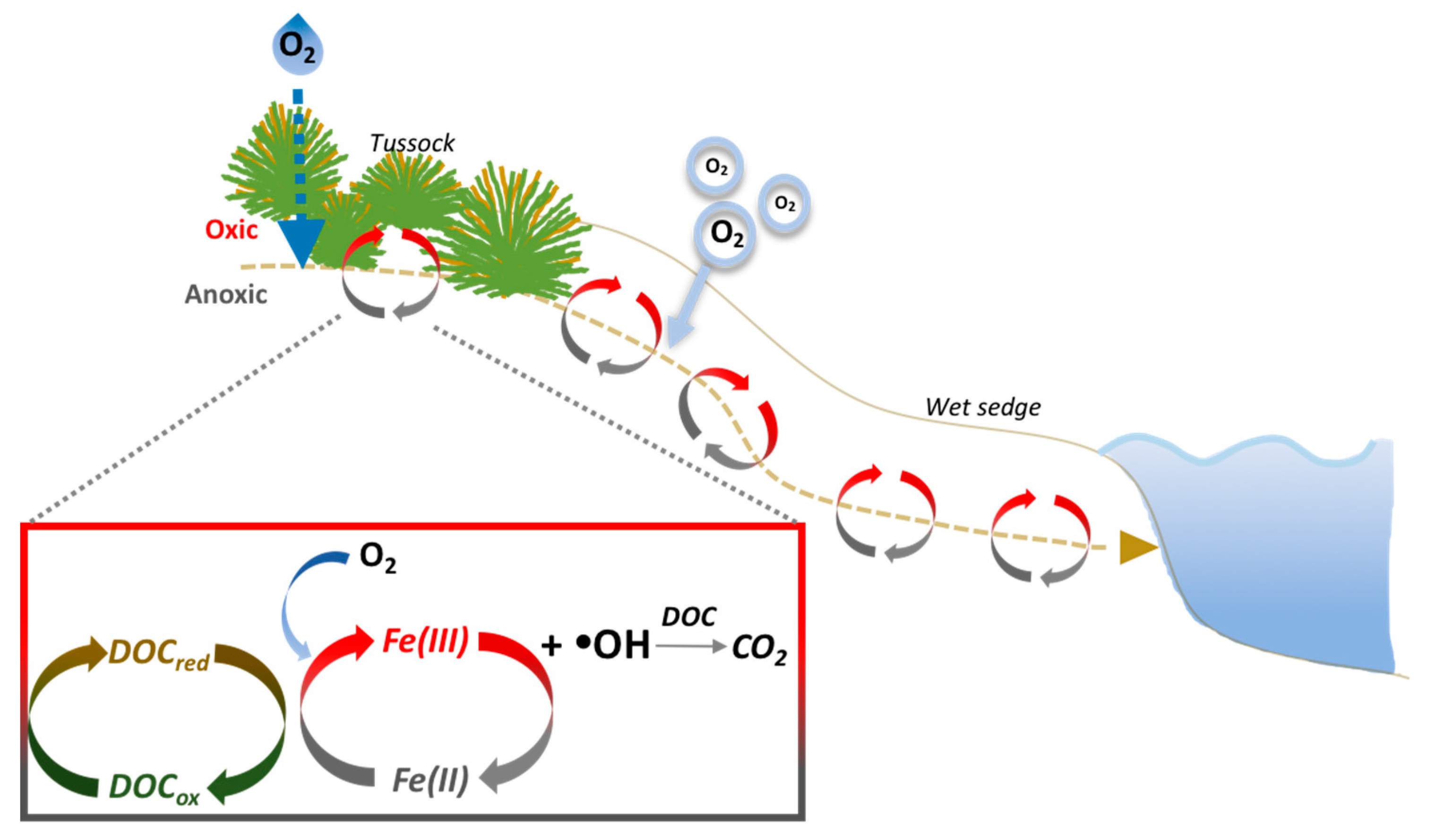
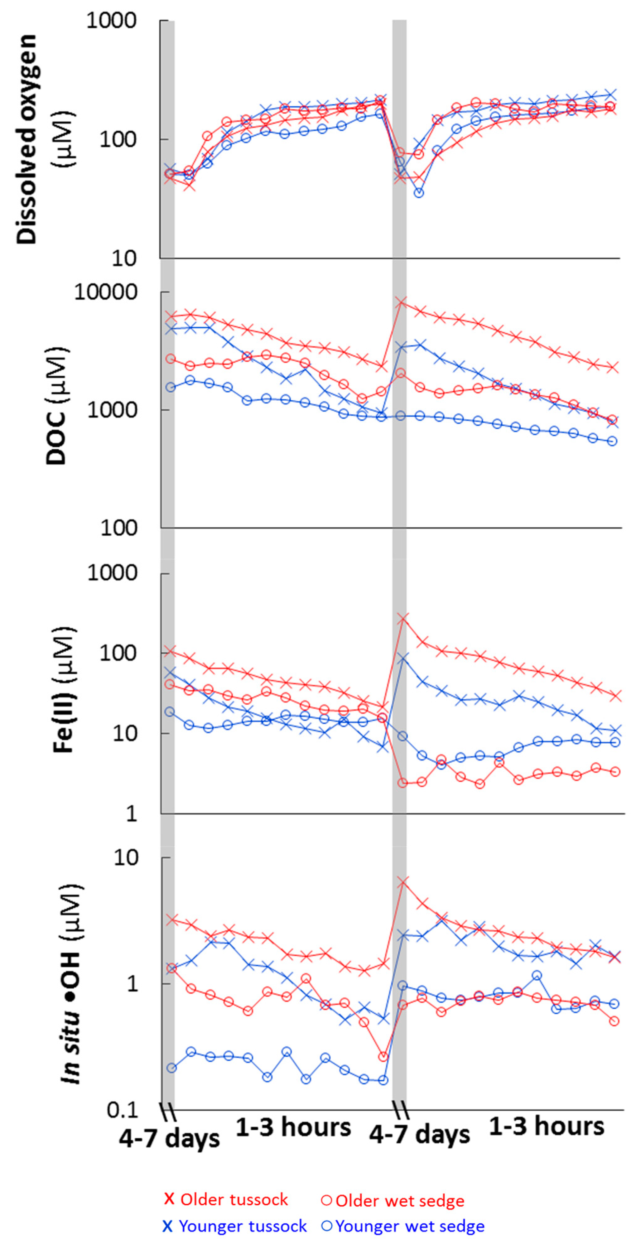
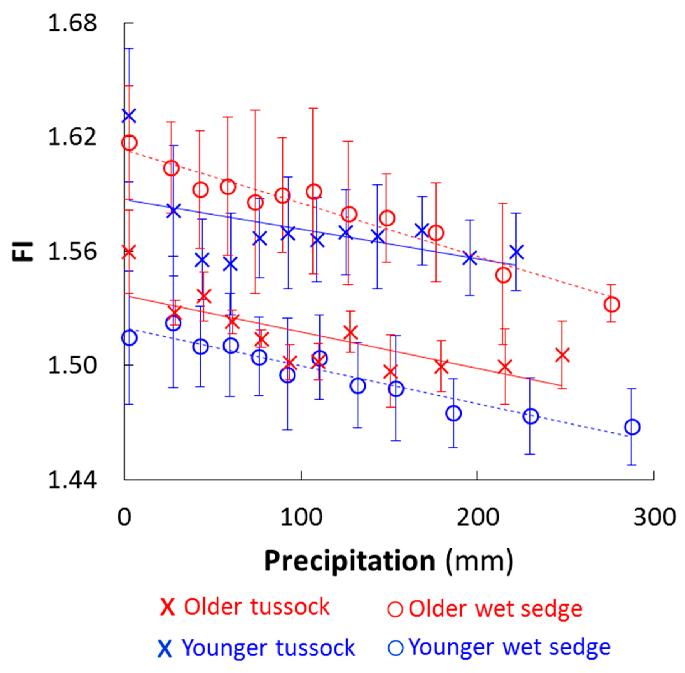
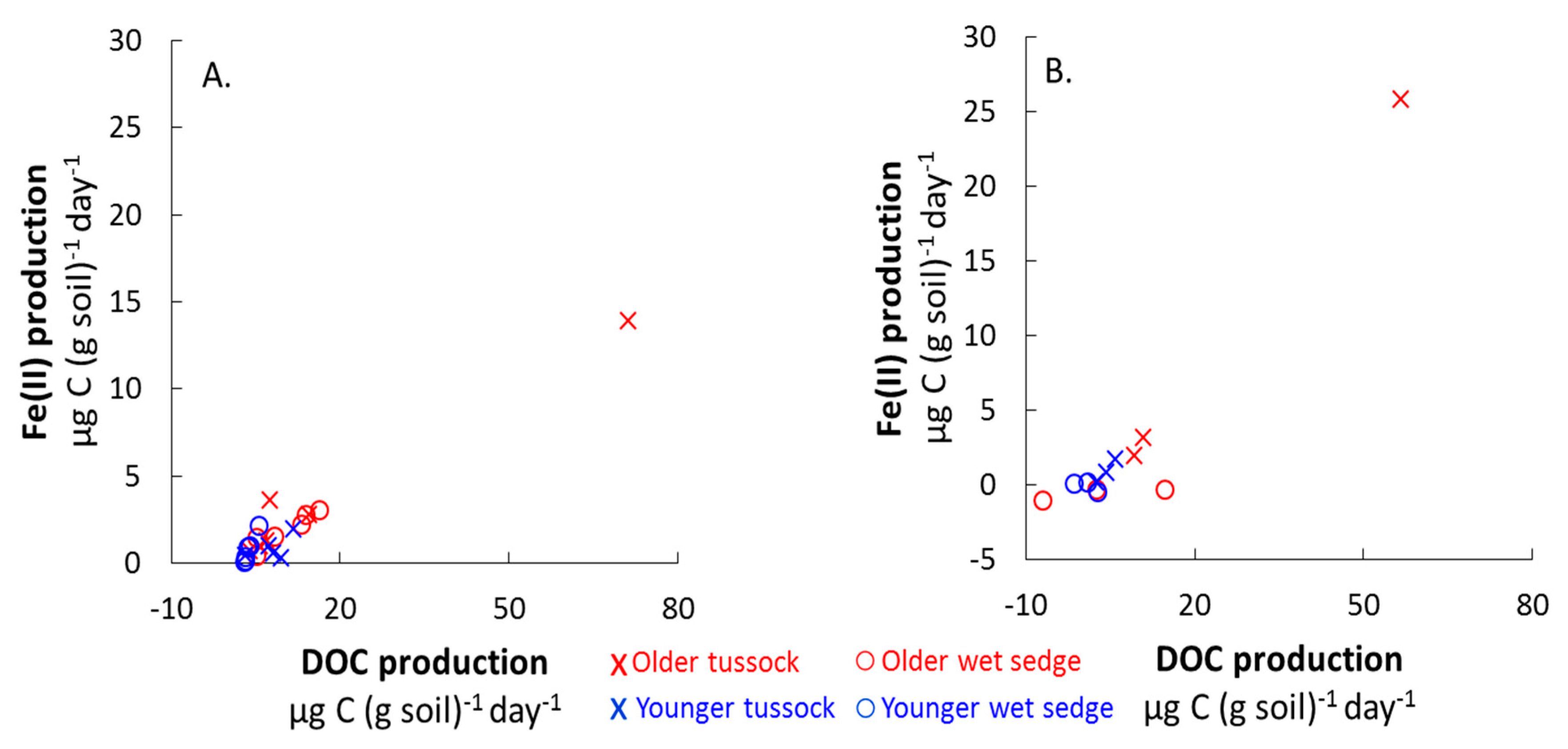
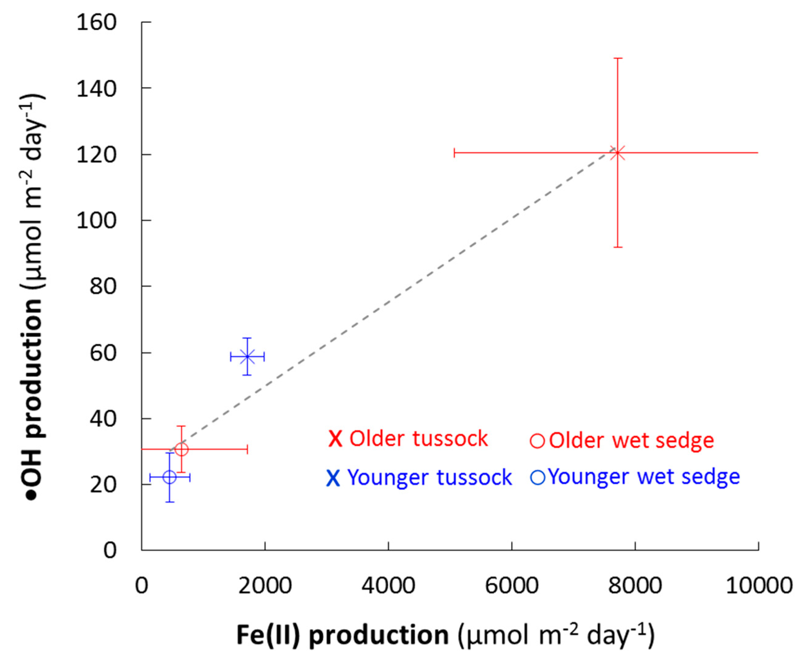
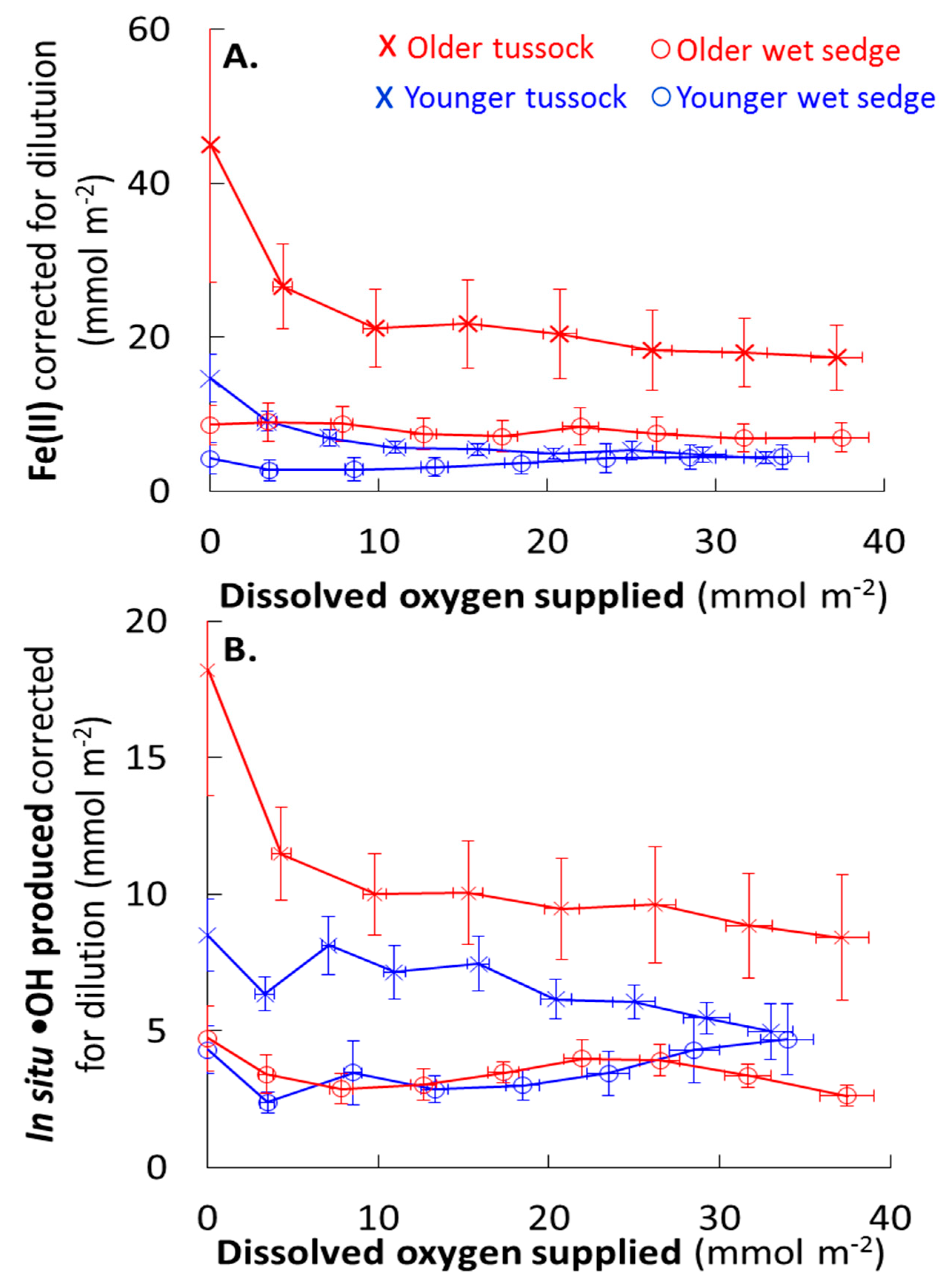
Table 1.
Properties of bulk soils of older and younger landscape age tussock and wet sedge mesocosms (average ± SE; N = 6) from the triplicate mesocosms of each landscape age and vegetation type measured after the second flushing period for the first experiment and after the only flushing period for the second experiment (Figure S1). Bulk density is the average bulk density of the soil core including organic and mineral layers. Soil moisture was quantified as the volumetric water content of the soils.
| Variable | Older (Imnavait) | Younger (Toolik) | ||||
|---|---|---|---|---|---|---|
| Vegetation | Tussock | Wet sedge | Tussock | Wet sedge | ||
| Horizon | Organic | Mineral | Organic | Organic | Mineral | Organic |
| Depth (cm) | 19 ± 8 | 9 ± 4 | 27 ± 1 | 15 ± 7 | 18 ± 8 | 30 ± 1 |
| Bulk density (g dry soil cm−3) | 0.3 ± 0.04 A | 0.2 ± 0.01 B | 0.4 ± 0.08 A | 0.2 ± 0.01 B | ||
| Soil organic carbon (%) | 40 ± 3 A | 5 ± 0 A | 40 ± 1 B,C | 30 ± 6 A | 6 ± 1 A | 35 ± 1 B,D |
| Moisture (% water) | 82 ± 3 A | 30 ± 2 A | 83.1 ± 1.2 B | 70 ± 7 B | 38 ± 5 B | 82 ± 0 B |
| Porosity (% of total soil volume) | 80 ± 3 A | 30 ± 2 A | 90 ± 6 B | 70 ± 7 B | 40 ± 5 B | 80 ± 6 B |
Letters A and B indicate significant differences (p < 0.05) between the same landscape ages but different vegetation types. Letters C and D indicate significant differences (p < 0.05) between different landscape ages and the same vegetation type.
Table 2.
Soil water chemistry for older and younger tussock and wet sedge soil waters (average ± SE, N = 9; Figure S1).
Table 2.
Soil water chemistry for older and younger tussock and wet sedge soil waters (average ± SE, N = 9; Figure S1).
| Variable | Older (Imnavait) | Younger (Toolik) | ||
|---|---|---|---|---|
| Vegetation | Tussock | Wet Sedge | Tussock | Wet Sedge |
| pH | 5.0 ± 0.1 A | 5.4 ± 0.1 B,C | 4.9 ± 0.1 A | 6.4 ± 0.1 B,D |
| Conductivity (µS cm−1) | 46 ± 3 | 34 ± 6 C | 44 ± 6 A | 151 ± 10 B,D |
| Dissolved oxygen (µM) | 47 ± 9 | 46 ± 4 | 49 ± 11 | 65 ± 12 |
| Electron donating capacity µmol (kg dry soil)−1 | 530 ± 210 C | 370 ± 90 | 120 ± 40 D | 190 ± 30 |
| DOC µg C (g dry soil)−1 | 120 ± 45 | 100 ± 16 C | 48 ± 7.1 | 49 ± 6.8 D |
| Fe(tot) µg (g dry soil)−1 | 22 ± 8.9 | 26 ± 6.2 C | 5.1 ± 1.2 | 11 ± 3.1 D |
| Fe(II) µg (g dry soil)−1 | 19 ± 7.5 C | 14 ± 3.0 C | 4.2 ± 1.2 D | 6.6 ± 2.6 D |
Letters A and B indicate significant differences (t-test, p < 0.05) between the same landscape ages but different vegetation types. Letters C and D indicate significant differences (t-test, p < 0.05) between different landscape ages and the same vegetation type.
Table 3.
Soil water DOC chemical characteristics based on absorbance and fluorescence (CDOM and FDOM, respectively) for older and younger tussock and wet sedge soils (average ± SE, N = 9, see Figure S1).
Table 3.
Soil water DOC chemical characteristics based on absorbance and fluorescence (CDOM and FDOM, respectively) for older and younger tussock and wet sedge soils (average ± SE, N = 9, see Figure S1).
| Variable | Older (Imnavait) | Younger (Toolik) | ||
|---|---|---|---|---|
| Vegetation | Tussock | Wet Sedge | Tussock | Wet Sedge |
| Slope ratio | 0.75 ± 0.05 C | 0.71 ± 0.01 | 0.86 ± 0.00 D | 0.77 ± 0.12 |
| Fluorescence Index | 1.56 ± 0.02 | 1.62 ± 0.03 C | 1.63 ± 0.04 A | 1.52 ± 0.02 B,D |
| C/A | 0.52 ± 0.02 | 0.55 ± 0.02 | 0.54 ± 0.03 | 0.51 ± 0.02 |
| T/A | 0.23 ± 0.08 C | 0.45 ± 0.20 | 0.63 ± 0.05 D | 1.06 ± 0.73 |
Letters A and B indicate significant differences (t-test, p < 0.05) between the same landscape ages but different vegetation types. Letters C and D indicate significant differences (t-test, p < 0.05) between different landscape ages and the same vegetation type.
Table 4.
EDC, DOC and iron production and O2 consumption in the soil waters of two landscape ages and vegetation types during the first acclimation period for both experiments (N = 6) and the second acclimation period for only the first experiment (N = 3; Figure S1).
Table 4.
EDC, DOC and iron production and O2 consumption in the soil waters of two landscape ages and vegetation types during the first acclimation period for both experiments (N = 6) and the second acclimation period for only the first experiment (N = 3; Figure S1).
| Variable | Older (Imnavait) | Younger (Toolik) | Older (Imnavait) | Younger (Toolik) | ||||
|---|---|---|---|---|---|---|---|---|
| Vegetation | Tussock | Wet sedge | Tussock | Wet sedge | Tussock | Wet sedge | Tussock | Wet sedge |
| Acclimation period | First | Second | ||||||
| Electron donating capacity production µmol (kg soil)−1 (day)−1 | 110 ± 57 | 60 ± 10 C,E | 24 ± 10 | 23 ± 4 D | 160 ± 120 | −1 ± 9 F | 20 ± 8 | 10 ± 7 |
| DOC production µg C (g soil)−1 (day)−1 | 18 ± 11 | 10 ± 1.9 C | 7.9 ± 1.4 A | 3.6 ± 0.4 B,D | 26 ± 16 | 3.3 ± 1.0 | 4.7 ± 0.9 A | 0.9 ± 1.4 B |
| Fe(tot) production g Fe (g soil)−1 (day)−1 | 4.5 ± 2.4 | 3.4 ± 0.8 C,E | 1.0 ± 0.3 | 1.3 ± 0.4 D | 11 ± 8.2 | −0.3 ± 0.4 C,F | 0.9 ± 0.3 | 0.6 ± 0.3 D |
| Fe(II) production µg Fe (g soil)−1 (day)−1 | 3.9 ± 2.1 C | 1.9 ± 0.4 C,E | 0.9 ± 0.1 D | 0.8 ± 0.3 D,E | 10 ± 7.8 | −0.5 ± 0.4 C,F | 0.9 ± 0.3 A | 0.1 ± 0.0 B,D,F |
| O2 consumption µg O2 (g soil)−1 (day)−1 | 3.0 ± 1.1 | 4.2 ± 0.3 C,E | 2.5 ± 0.5 | 2.8 ± 0.4 D | 2.1 ± 1.2 | 2 ± 0.9 F | 1.9 ± 0.8 | 2.6 ± 0.9 |
Letters A and B indicate significant differences (t-test; p < 0.05) between the same landscape ages but different vegetation types. Letters C and D indicate significant differences (t-test, p < 0.05) between different landscape ages and the same vegetation type. Letters E and F indicate significant differences (t-test, p < 0.05) between the first and second flushing period for the same landscape age and vegetation type (N = 3; Figure S1).
Table 5.
•OH production rates during precipitation events (flushing period) and under waterlogged, low O2 conditions (acclimation period) (average ± SE, N = 9; Figure S1). •OH production rates during precipitation events were calculated using the yield of •OH per O2 supplied with the first flush times the amount of O2 supplied during a 4 mm per day rain event (an average precipitation event in the Arctic). •OH production rates during waterlogged, low O2 conditions were calculated as the •OH concentration in soil water collected after the acclimation period divided by the number of days of the acclimation period. The summer time production of •OH and CO2 from the oxidation of DOC by •OH were calculated by multiplying the daily rates by the number of days during a summer (on average) that are rainy (67 days) or characterized by static, waterlogged conditions (73 days).
| Daily Production Rate | Precipitation Events | Waterlogged Soils |
|---|---|---|
| •OH (µmol m−2 day−1) | 200 ± 70 A | 60 ± 20 B |
| CO2 (µmol m−2 day−1) | 60 ± 20 A | 20 ± 6 B |
| Summer time production | ||
| •OH (mmol m−2) | 10 ± 5 | 4 ± 1 |
| CO2 (mmol m−2) | 4 ± 1 A | 1 ± 0.4 B |
Letters A and B indicate significant differences (t-test, p < 0.05) between the •OH and CO2 production during precipitation event and under waterlogged conditions.
© 2018 by the authors. Licensee MDPI, Basel, Switzerland. This article is an open access article distributed under the terms and conditions of the Creative Commons Attribution (CC BY) license (http://creativecommons.org/licenses/by/4.0/).
Share and Cite
MDPI and ACS Style
Trusiak, A.; Treibergs, L.A.; Kling, G.W.; Cory, R.M. The Controls of Iron and Oxygen on Hydroxyl Radical (•OH) Production in Soils. Soil Syst. 2019, 3, 1. https://0-doi-org.brum.beds.ac.uk/10.3390/soilsystems3010001
AMA Style
Trusiak A, Treibergs LA, Kling GW, Cory RM. The Controls of Iron and Oxygen on Hydroxyl Radical (•OH) Production in Soils. Soil Systems. 2019; 3(1):1. https://0-doi-org.brum.beds.ac.uk/10.3390/soilsystems3010001
Chicago/Turabian StyleTrusiak, Adrianna, Lija A. Treibergs, George W. Kling, and Rose M. Cory. 2019. "The Controls of Iron and Oxygen on Hydroxyl Radical (•OH) Production in Soils" Soil Systems 3, no. 1: 1. https://0-doi-org.brum.beds.ac.uk/10.3390/soilsystems3010001