Distributed Complementary Control Research of Wind Turbines in Two Offshore Wind Farms

Abstract

In order to stabilize the fluctuation of wind power and maintain a stable power output, a complementary control idea is proposed. This idea aims to make the output power from two wind farms complement each other. This study proposes a distributed control strategy to solve the complementary control problem of wind turbines in two offshore wind farms on the basis of the Hamiltonian energy theory. The proposed control strategy not only ensures synchronization for wind turbines in the same farm but also keeps the combined output power of the two wind farms stable. First, through the Hamiltonian realization, the single-machine model of a wind turbine is transformed into a port-controlled Hamiltonian system with dissipation (PCHD). Subsequently, the Hamiltonian energy control law is developed on the basis of the energy-shaping method to adjust the Hamiltonian energy function. The complementary control of the two wind farms is designed to synchronize the wind turbines within an individual wind farm and keep the combined output of the two wind farms stable. Furthermore, the complementary control strategy is modified to address the communication delay between the two wind farms by incorporating time delay into the control problem. Finally, the effectiveness of the distributed complementary control has been verified via simulations.

1. Introduction

Recently, offshore wind-power generation has been receiving considerable attention from various countries because of its advantages, such as abundant reserves, a high energy-utilization rate, and the fact that wind power does not require land resources. In eastern China, the load requirements are relatively high for the developed regions along the coastlines. Thus, offshore wind power has been rapidly developed [1,2,3,4]. Unlike onshore wind farms, offshore wind farms are located far away from the land, which makes maintenance fairly difficult. As a result, higher reliability and autonomy are essential for offshore wind farms. Furthermore, with the expansion of capacity and the increase in offshore distance, offshore wind power is facing an increasing number of problems. Therefore, new control methods and designs are required to solve these growing problems associated with offshore wind-power generation [5,6,7].

The sea contains abundant wind resources. However, because of its complicated environment and constant changes in wind speed, achieving stability of the power produced by offshore wind turbines is a challenge for researchers. When the wind potential of a wind farm changes, its output electrical energy transmitted to the power grid is also affected. In this study, we aim to stabilize the output power of two wind farms using the proposed control strategy. When the output power of a wind farm decreases, the other farm can compensate for the loss of power. Hence, the sum of the output power will be maintained largely at a stable level, which can reduce the requirements for energy storage and adjusting thermal power.

An offshore wind farm consists of dozens of wind turbines, wherein each wind turbine is regarded as a network node, and the communication lines between the wind turbines are regarded as links between the nodes. Hence, an offshore wind farm can be perceived as a distributed network. The traditional centralized paradigm has conceptual advantages but also inherent limitations [8,9]. The practice in the wind industry relies on distributed control structures, and there is a strong need for more systematic approaches for the design of such controllers, taking the distributed information into account. Distributed control can effectively solve the control problems of a networked system. By exchanging information between the wind turbines, the distributed control strategy is formulated on the basis of the information obtained by each unit from its neighbouring units, thereby effectively realizing the control of the entire distributed network. Therefore, distributed control has been considered as a promising technique to be applied in offshore wind farms [10,11]. Furthermore, the consensus problem is the basis of the distributed control of multi-agent systems [12,13]. On the basis of satisfying the output consensus of wind turbines in wind farms, complementary control is proposed as an extension study, to alleviate the impact of power fluctuation on the grid.

Stochastically fluctuating wind power has a negative impact on power grid operations. How to smooth the power fluctuation and minimize the output impact on the grid is always the focus of attention. Jiang et al. proposed a wind-power filtering approach in order to mitigate short- and long-term fluctuations using a hybrid energy storage system [14]. Li et al. presented coordinated control strategies to improve system inertia through exerting capacitor energy and minimizing the impact on wind energy harvesting with the aid of communication between onshore and offshore grids [15]. For offshore wind power plants integrated to a three-terminal high-voltage direct current (DC) system, a coordinated fast primary frequency control scheme was proposed. Furthermore, the impact of wind-speed variation on the active power output and the AC grid frequency was analyzed in [16]. Our work solves this problem by taking advantage of the natural complementary characteristics of wind energy. Offshore wind farms are normally located far away from each other, in areas with different wind conditions. In order to keep the total output stable and minimize the power impact on the power grid, through coordinating two wind farms with complementary characteristics, this study proposes a distributed complementary control strategy to synchronize the output of the wind turbines within the individual wind farm and maintain the combined power of the two wind farms at a stable level. Moreover, the communication delay between two offshore farms due to the considerable distance is considered, and the complementary control problem with time delay is also investigated in this study.

The Hamiltonian energy method provides a framework with a nice structure and clear physical meaning for nonlinear control systems [17]. With the method, many significant achievements have been obtained for single- and multi-machine systems [18,19]. Nevertheless, without considering network graphs, these multi-machine systems are not regarded as distributed systems. This paper proposes a distributed control strategy based on the Hamiltonian energy method. In this study, the wind turbine is formulated as a port-controlled Hamiltonian system with dissipation (PCHD) through the Hamiltonian realization. Additionally, the Hamiltonian energy function of the system is modified by using the energy-shaping method [20]. The detailed procedures of this study are as follows: first, a single-machine model of the wind turbine is realized in the PCHD form, and it is further expanded to the Hamiltonian model of a wind turbine farm. Second, the complementary control problem of the two wind farms is investigated. The complementary control is designed by introducing the coordination controller. When a communication link between the two wind farms exists, distributed complementary control helps the two farms achieve the objectives of individual and combined output stabilization. Furthermore, the communication delay between the two wind farms is considered, and a modified control strategy is proposed to solve the control problem of the system with time delay. Finally, the feasibility of the complementary control strategy has been verified via simulations. Under normal conditions, the complementary control helps to maintain the stability of the combined output power of the two wind farms. In case of failure, or even if a unit breaks down, the complementary control strategy can keep the total output power stable.

In conclusion, the main goal or contribution of this study includes the following aspects. First, the objective of distributed complementary control is to smoothen the fluctuation of power and keep a output stable in order to reduce the impact on the grid and relieve the pressure of power scheduling. Second, distributed complementary control is proposed to solve the cooperative control problem of two wind farms, which extends to distributed control from a single wind farm to multiple wind farms. Third, considering that the communication delay is non-negligible for long distances between two wind farms, the complementary control is extended to the system with a time delay.

The organization of this paper is as follows. In Section 2, the single-machine Hamiltonian realization of a wind turbine is introduced. In Section 3, the complementary control strategy of two wind farms is proposed. In Section 4, the control strategy with the communication delay is designed. In Section 5, the simulation results verify the effectiveness of the design approach. Finally, Section 6 provides the conclusions.

2. Single-Machine Hamiltonian Realization of Wind Turbine

The single-machine Hamiltonian realization of a wind turbine is given in this section, and it is considered as the basic model for the Hamiltonian model of a wind farm in Section 3. In this study, the doubly fed wind turbine is represented as the following third-order model [21,22,23]:

$$\begin{array}{c}\hfill \left\{\begin{array}{ccc}\hfill 2H_{tot}\frac{ds}{dt}& \hfill =& P_s-P_m=-E_d^{{}^{\prime }}{i}_{ds}-E_q^{{}^{\prime }}{i}_{qs}-P_m\hfill \\ \hfill \frac{d{E}_q^{{}^{\prime }}}{dt}& \hfill =& -s{\omega }_s{E}_d^{{}^{\prime }}-\frac{1}{T_0^{{}^{\prime }}}\left[E_q^{{}^{\prime }}-(X_s-X_s^{{}^{\prime }})i_{ds}\right]+{\omega }_s\frac{L_m}{L_{rr}}{v}_{dr}\hfill \\ \hfill \frac{d{E}_d^{{}^{\prime }}}{dt}& \hfill =& s{\omega }_s{E}_q^{{}^{\prime }}-\frac{1}{T_0^{{}^{\prime }}}\left[E_d^{{}^{\prime }}+(X_s-X_s^{{}^{\prime }})i_{qs}\right]-{\omega }_s\frac{L_m}{L_{rr}}{v}_{qr}\hfill \end{array}\right.\end{array}$$

(1)

where $X_s={\omega }_s{L}_{ss}$, $X_s^{{}^{\prime }}={\omega }_s(L_{ss}-\frac{L_m^2}{L_{rr}})$, $T_0^{{}^{\prime }}=\frac{L_{rr}}{R_r}$, s is the rotor’s slip ratio, $H_{tot}$ is the inertia constant of the wind turbine and the generator, and $P_s=-E_d^{{}^{\prime }}{i}_{ds}-E_q^{{}^{\prime }}{i}_{qs}$ is the active power output of the stator of the wind turbine. $Q_s=E_d^{{}^{\prime }}{i}_{qs}-E_q^{{}^{\prime }}{i}_{ds}$ is the reactive power output of the stator of the wind turbine, $P_m$ is the mechanical power input of the wind turbine, $L_{ss}$ is the self-inductance of the stator, $L_{rr}$ is the self-inductance of the rotor, $L_m$ is the mutual inductance, and $R_r$ is the resistance of the rotor; ${\omega }_s$ is the synchronous speed, $X_s$ is the reactance of the stator, $X_s^{{}^{\prime }}$ is the transient reactance of the stator, and $i_{ds}$ and $i_{qs}$ are the currents of the stator along the d- and q-axes, respectively. $E_d^{{}^{\prime }}$ and $E_q^{{}^{\prime }}$ are the voltages of the transient reactance along the d- and q-axes, respectively, and $v_{dr}$ and $v_{qr}$ are the voltages of the rotor along the d- and q-axes, respectively. Hence, Equation (1) is a double-input, third-order model of the wind turbine under the d–q coordinate system, where s, $E_d^{{}^{\prime }}$ and $E_q^{{}^{\prime }}$ are the state variables, and $v_{dr}$ and $v_{qr}$ are the input variables.

First, the Hamiltonian energy function can be constructed as follows:

$$\begin{array}{c}\hfill H=\frac{s^2}{2}+\frac{1}{2}{\left(E_q^{{}^{\prime }}+\frac{P_m}{2i_{qs}}\right)}^2+\frac{1}{2}{\left(E_d^{{}^{\prime }}+\frac{P_m}{2i_{ds}}\right)}^2\end{array}$$

(2)

Consequently, the system described by Equation (1) can be transformed into the port-controlled Hamiltonian (PCH) system as follows:

$$\begin{array}{ccc}\hfill \frac{d}{dt}\left[\begin{array}{c}s\\ E_q^{{}^{\prime }}\\ E_d^{{}^{\prime }}\end{array}\right]& =& \left[\begin{array}{ccc}0& -\frac{i_{qs}}{2H_{tot}}& -\frac{i_{ds}}{2H_{tot}}\\ 0& -\frac{1}{T_0^{{}^{\prime }}}& -s{\omega }_s\\ 0& s{\omega }_s& -\frac{1}{T_0^{{}^{\prime }}}\end{array}\right]\nabla H+\left[\begin{array}{c}0\\ \frac{i_{ds}}{T_0^{{}^{\prime }}}(X_s-X_s^{{}^{\prime }})+\frac{P_m}{2T_0^{{}^{\prime }}{i}_{qs}}+s{\omega }_s\frac{P_m}{2i_{ds}}\\ -\frac{i_{qs}}{T_0^{{}^{\prime }}}(X_s-X_s^{{}^{\prime }})+\frac{P_m}{2T_0^{{}^{\prime }}{i}_{ds}}-s{\omega }_s\frac{P_m}{2i_{qs}}\end{array}\right]\hfill \\ & & +\left[\begin{array}{cc}0& 0\\ {\omega }_s\frac{L_m}{L_{rr}}& 0\\ 0& -{\omega }_s\frac{L_m}{L_{rr}}\end{array}\right]\left[\begin{array}{c}{v}_{dr}\\ v_{qr}\end{array}\right]\hfill \end{array}$$

(3)

Second, the PCH system is transformed into the PCHD system through a pre-feedback control. The whole controller can be developed using the following equation:

$$\begin{array}{c}\hfill u=\left[\begin{array}{c}{v}_{dr}\\ v_{qr}\end{array}\right]=K+\mu =\left[\begin{array}{c}{K}_{dr}\\ K_{qr}\end{array}\right]+\left[\begin{array}{c}{\mu }_{dr}\\ {\mu }_{qr}\end{array}\right]\end{array}$$

(4)

where the control law is divided into two parts: the pre-feedback controller K and the output feedback controller $\mu$. Hence,

$$\begin{array}{c}\hfill K=\left[\begin{array}{c}{K}_{dr}\\ K_{qr}\end{array}\right]=\left[\begin{array}{c}-\frac{L_{rr}}{{\omega }_s{L}_m}\left(\frac{i_{ds}}{T_0^{{}^{\prime }}}(X_s-X_s^{{}^{\prime }})+\frac{P_m}{2T_0^{{}^{\prime }}{i}_{qs}}+\left(\frac{{\omega }_s{P}_m}{2i_{ds}}-\frac{i_{qs}}{2H_{tot}}\right)s\right)\\ \frac{L_{rr}}{{\omega }_s{L}_m}\left(-\frac{i_{qs}}{T_0^{{}^{\prime }}}(X_s-X_s^{{}^{\prime }})+\frac{P_m}{2T_0^{{}^{\prime }}{i}_{ds}}-\left(\frac{{\omega }_s{P}_m}{2i_{qs}}+\frac{i_{ds}}{2H_{tot}}\right)s\right)\end{array}\right]\end{array}$$

(5)

The closed-loop system can be rewritten as a PCHD model:

$$\begin{array}{ccc}\hfill \frac{d}{dt}\left[\begin{array}{c}s\\ E_q^{{}^{\prime }}\\ E_d^{{}^{\prime }}\end{array}\right]& =& \left[\begin{array}{ccc}0& -\frac{i_{qs}}{2H_{tot}}& -\frac{i_{ds}}{2H_{tot}}\\ \frac{i_{qs}}{2H_{tot}}& -\frac{1}{T_0^{{}^{\prime }}}& -s{\omega }_s\\ \frac{i_{ds}}{2H_{tot}}& s{\omega }_s& -\frac{1}{T_0^{{}^{\prime }}}\end{array}\right]\nabla H+\left[\begin{array}{cc}0& 0\\ {\omega }_s\frac{L_m}{L_{rr}}& 0\\ 0& -{\omega }_s\frac{L_m}{L_{rr}}\end{array}\right]\left[\begin{array}{c}{\mu }_{dr}\\ {\mu }_{qr}\end{array}\right]\hfill \\ & \stackrel{▵}{=}& (J-R)\nabla H+G\mu \hfill \end{array}$$

(6)

where $J=\left[\begin{array}{ccc}0& -\frac{i_{qs}}{2H_{tot}}& -\frac{i_{ds}}{2H_{tot}}\\ \frac{i_{qs}}{2H_{tot}}& 0& -s{\omega }_s\\ \frac{i_{ds}}{2H_{tot}}& s{\omega }_s& 0\end{array}\right]$, $R=\left[\begin{array}{ccc}0& 0& 0\\ 0& \frac{1}{T_0^{{}^{\prime }}}& 0\\ 0& 0& \frac{1}{T_0^{{}^{\prime }}}\end{array}\right]$, $G=\left[\begin{array}{cc}0& 0\\ {\omega }_s\frac{L_m}{L_{rr}}& 0\\ 0& -{\omega }_s\frac{L_m}{L_{rr}}\end{array}\right]$

Thus, Equation (6) matches the PCHD form. The output equation is expressed as

$$\begin{array}{c}\hfill y=G^T\nabla H=\left[\begin{array}{c}{\omega }_s\frac{L_m}{L_{rr}}(E_q^{{}^{\prime }}+\frac{P_m}{2i_{qs}})\\ -{\omega }_s\frac{L_m}{L_{rr}}(E_d^{{}^{\prime }}+\frac{P_m}{2i_{ds}})\end{array}\right]\end{array}$$

(7)

3. Complementary Control Strategy of Wind Farms

3.1. Graph Theory of Network Topology

An offshore wind farm can be seen as a distributed network, wherein the wind turbines are regarded as the nodes and exchange information through the communication lines. On the basis of this network, the distributed control strategy of the whole system has been developed. The terms associated with the graph theory are given as follows [24]:

Consider n nodes that interact with each other. The relationship between them can be expressed as a directed or undirected graph. A graph $G(V,E)$ consists of a node set $V=\{v_1,v_2,\dots ,v_n\}$ and an edge set $E\subseteq V\times V$. If the edge of the graph is an unordered pair of nodes, $(v_i,v_j)=(v_j,v_i)$, where $i,j=1,2,\dots ,n$, the graph is considered undirected. Similarly, if the edge of the graph is an ordered pair of nodes, $(v_i,v_j)\ne (v_j,v_i)$, the graph is considered as directed. $A=\left[a_{ij}\right]$ is the adjacency matrix. When $(v_j,v_i)\in E$, $a_{ij}>0$; otherwise $a_{ij}=0$. The neighbouring nodes of $v_i$ can be expressed as $N_i=\{v_j:(v_j,v_i)\in E\}$. The in-degree $d_i$ (i.e., the sum of the elements of the ith row of matrix A) of node i is defined as $d_i={\sum }_{j\in N_i}{a}_{ij}$. Subsequently, the in-degree matrix is defined as $D=diag\left\{d_i\right\}$, and the Laplacian matrix L is defined as $L=D-A$. If a path between any two nodes, in an undirected graph, can always be determined, then this graph is called a connected graph. In the case of a directed graph, it is called a strongly connected graph. Considering a directed graph, if every node except the root node has only one parent node, the directed graph is a directed tree. If a directed graph contains a directed tree, this directed tree is called a directed spanning tree to a directed graph. The following is an important lemma on the directed graph:

Lemma 1

([25]). Suppose that $z={[z_1^T,\dots ,z_p^T]}^T$ with $z_i\in {\mathbf{R}}^m$ and $L_p\in {\mathbf{R}}^{p\times p}$ is the Laplacian matrix of a directed graph. Then the following five conditions are equivalent:

(1) 

The directed graph of $L_p$ has a directed spanning tree.

(2) 

$(L_p\otimes I_m)z=0$, which implies that $z_1=\dots =z_p$.

(3) 

$L_p$ has a simple zero eigenvalue with an associated eigenvector $1_p$, and all other eigenvalues have positive real parts.

(4) 

Consensus is reached asymptotically for the system $\dot{z}=-(L_p\otimes I_m)z$.

(5) 

The rank of $L_p$ is $p-1$.

3.2. Description of the Complementary Control Problem of Wind Farms

In this subsection, the PCHD model given in Equation (6) is extended into the model of wind turbines in wind farms, on the basis of graph theory.

$$\begin{array}{c}\hfill \left\{\begin{array}{ccc}\hfill {\dot{x}}_i& \hfill =& (J_i-R_i)\nabla H_i\left(x_i\right)+G_i{\mu }_i\hfill \\ \hfill y_i& \hfill =& G_i^T\nabla H_i\left(x_i\right)\hfill \end{array}\right.i=1,\cdots ,N\end{array}$$

(8)

where the state of the ith wind turbine is $x_i={\left[\begin{array}{ccc}{s}_i& E_{qi}^{{}^{\prime }}& E_{di}^{{}^{\prime }}\end{array}\right]}^T$, and the input is ${\mu }_i=\left[\begin{array}{c}{\mu }_{dri}\\ {\mu }_{qri}\end{array}\right]$. The gradient of the Hamiltonian energy function $H_i$ is $\nabla H_i={\left[\begin{array}{ccc}{s}_i& E_{qi}^{{}^{\prime }}+\frac{P_{mi}}{2i_{qsi}}& E_{di}^{{}^{\prime }}+\frac{P_{mi}}{2i_{dsi}}\end{array}\right]}^T$, and the output is $y_i=\left[\begin{array}{c}{\omega }_{si}\frac{L_{mi}}{L_{rri}}\left(E_{qi}^{{}^{\prime }}+\frac{P_{mi}}{2i_{qsi}}\right)\\ -{\omega }_{si}\frac{L_{mi}}{L_{rri}}\left(E_{di}^{{}^{\prime }}+\frac{P_{mi}}{2i_{dsi}}\right)\end{array}\right]$. $J_i$, $R_i$ and $G_i$ are the same as J, R, and G in Equation (6), respectively. The only difference between them is that $J_i$, $R_i$ and $G_i$ have the index i with each variable, which represents the parameters of the ith wind turbine.

Referring to the definition of group consistency [26], the output complementation of the system, Equation (8), is defined as follows:

Definition 1.

For the networked system given in Equation (8), consisting of N PCHD nodes in two wind farms, $A_1=\{i_1,i_2,\dots ,i_n\}\subset \{1,2,\dots ,N\}$, $A_2=\{1,2,\dots ,N\}\setminus A_1$, and $T={\left[\begin{array}{cc}{T}_{01}& T_{02}\end{array}\right]}^T$ is a constant vector. If the outputs of the N PCHD nodes satisfy the following conditions:

$$\begin{array}{c}\underset{t\to \infty }{lim}\parallel y_j\left(t\right)-y_k\left(t\right)\parallel =0,\forall j,k\in A_1\hfill \end{array}$$

(9)

$$\begin{array}{c}\underset{t\to \infty }{lim}\parallel y_j\left(t\right)-y_k\left(t\right)\parallel =0,\forall j,k\in A_2\hfill \end{array}$$

(10)

$$\begin{array}{c}\underset{t\to \infty }{lim}(y_j\left(t\right)+y_k\left(t\right))=T,\forall j\in A_1,k\in A_2\hfill \end{array}$$

(11)

where $\parallel ·\parallel$ is the Euclidean norm, the outputs of the wind farms $A_1$ and $A_2$ complement each other, and T is the target value.

Remark 1.

The output active power of the wind turbine is

$$\begin{array}{c}\hfill P_s=-E_d^{{}^{\prime }}{i}_{ds}-E_q^{{}^{\prime }}{i}_{qs}=\frac{L_{rr}}{{\omega }_s{L}_m}(i_{ds}{y}_2-i_{qs}{y}_1)+P_m\end{array}$$

Hence,

$$\begin{array}{c}\hfill \left\{\begin{array}{ccc}\hfill P_{sj}& \hfill =& \frac{L_{rrj}}{{\omega }_{sj}{L}_{mj}}(i_{dsj}{y}_{j2}-i_{qsj}{y}_{j1})+P_{mj},j\in A_1\hfill \\ \hfill P_{sk}& \hfill =& \frac{L_{rrk}}{{\omega }_{sk}{L}_{mk}}(i_{dsk}{y}_{k2}-i_{qsk}{y}_{k1})+P_{mk},k\in A_2\hfill \end{array}\right.\end{array}$$

(12)

When the outputs of the wind turbines in each wind farm are synchronized and the active powers of the two farms are complementary to each other, we have

$$\begin{array}{c}\hfill y_j+y_k=\left[\begin{array}{c}{y}_{j1}+y_{k1}\\ y_{j2}+y_{k2}\end{array}\right]=T=\left[\begin{array}{c}{T}_{01}\\ T_{02}\end{array}\right]\end{array}$$

Supposing that the main parameters of these units approximately coincide and that the two wind farms have the same number of wind turbines, $N=2n$, the sum of the output active power of the two wind farms is

$$\begin{array}{ccc}\hfill P_{sA}& =& P_{s{A}_1}+P_{s{A}_2}=\sum _{j\in A_1}{P}_{sj}+\sum _{k\in A_2}{P}_{sk}\hfill \\ & =& \frac{n{L}_{rr}}{{\omega }_s{L}_m}[i_{ds}(y_{j2}+y_{k2})-i_{qs}(y_{j1}+y_{k1})]+\sum _{i\in A_1+A_2}{P}_{mi}\hfill \\ & =& \frac{n{L}_{rr}}{{\omega }_s{L}_m}(i_{ds}{T}_{02}-i_{qs}{T}_{01})+\sum _{i\in A_1+A_2}{P}_{mi}\hfill \end{array}$$

(13)

This means that when the outputs of the wind farms are complementary to each other, the active powers of the two wind farms can also be complementary to each other, and their sum remains constant. Moreover, if the total output active power $P_{sA}$ is known, we can find a corresponding T satisfying Equation (13) and design the corresponding complementary control strategy to make the total output active power achieve the target value.

3.3. Complementary Control Design of Wind Farms

The complementary control strategy includes two steps: first, adjusting the Hamiltonian energy function $H_i\left(x_i\right)$ to the new energy function $H_{id}\left(x_i\right)$ through the Hamiltonian energy-shaping method. Second, developing the complementary control strategy using the new energy function.

Assuming $e_i=\left\{\begin{array}{c}\hfill 1,i\in A_1\\ \hfill 2,i\in A_2\end{array}\right.$, the outputs of the wind turbines need to satisfy

$$\begin{array}{c}\hfill G_i^T\nabla H_{id}\left(x_i\right)=y_i-T_{e_i}\end{array}$$

(14)

where $T_{e_i}$ is the modified output. $T_1={\left[\begin{array}{cc}{T}_{11}& T_{12}\end{array}\right]}^T$ and $T_2={\left[\begin{array}{cc}{T}_{21}& T_{22}\end{array}\right]}^T$; $T=T_1+T_2$ is the target value. We let the energy-shaping control law be ${\overline{\mu }}_i$. Consequently, the system under the action of ${\overline{\mu }}_i$ can be rewritten as

$$\begin{array}{c}\hfill (J_i-R_i)\nabla H_i\left(x_i\right)+G_i{\overline{\mu }}_i=(J_i-R_i)\nabla H_{id}\left(x_i\right)\end{array}$$

(15)

Hence,

$$\begin{array}{c}\hfill G_i{\overline{\mu }}_i=-(J_i-R_i)(\nabla H_i\left(x_i\right)-\nabla H_{id}\left(x_i\right))\end{array}$$

(16)

The following matching conditions should be satisfied:

$$\begin{array}{c}\hfill G_i^{\perp }(J_i-R_i)(\nabla H_i\left(x_i\right)-\nabla H_{id}\left(x_i\right))=0\end{array}$$

where $G_i^{\perp }$ is a nonsingular left annihilator satisfying $G_i^{\perp }{G}_i=0$.

We note that $G_i$ (Equation (16)) represents a column full-rank matrix. The energy-shaping control can be expressed as follows:

$$\begin{array}{c}\hfill {\overline{\mu }}_i=-{\left(G_i^T{G}_i\right)}^{-1}{G}_i^T(J_i-R_i)(\nabla H_i\left(x_i\right)-\nabla H_{id}\left(x_i\right))\end{array}$$

(17)

By summarizing the aforementioned analyses, the following theorem is obtained.

Theorem 1.

For wind turbines in offshore wind farms, on the basis of the energy-shaping method, the Hamiltonian energy control law is defined as

$$\begin{array}{c}\hfill {\mu }_i={\overline{\mu }}_i+{\tilde{\mu }}_i=-\frac{L_{rri}^2}{{\omega }_{si}^2{L}_{mi}^2}\left[\begin{array}{c}-\frac{T_{e_{i}1}}{T_{0i}^{{}^{\prime }}}+s_i{\omega }_{si}{T}_{e_{i}2}\\ -s_i{\omega }_{si}{T}_{e_{i}1}-\frac{T_{e_{i}2}}{T_{0i}^{{}^{\prime }}}\end{array}\right]+\left[\begin{array}{c}{\tilde{\mu }}_{dri}\\ {\tilde{\mu }}_{qri}\end{array}\right]\end{array}$$

(18)

where ${\tilde{\mu }}_i=\left[\begin{array}{c}{\tilde{\mu }}_{dri}\\ {\tilde{\mu }}_{qri}\end{array}\right]$ is the coordinated controller to be designed in the subsequent study. Using Equation (17), the system satisfies the condition of Equation (14) via the new Hamiltonian energy function $H_{id}\left(x_i\right)$.

Proof of Theorem 1.

According to Equation (14), the desired Hamiltonian function $H_{id}\left(x_i\right)$ needs to be developed from

$$\begin{array}{c}\hfill G_i^T\nabla H_{id}\left(x_i\right)=G_i^T\nabla H_i\left(x_i\right)-T_{e_i}\end{array}$$

Consequently,

$$\begin{array}{c}\hfill \nabla H_i\left(x_i\right)-\nabla H_{id}\left(x_i\right)={\left(G_i{G}_i^T\right)}^{-1}{G}_i{T}_{e_i}=\frac{L_{rri}}{{\omega }_{si}{L}_{mi}}\left[\begin{array}{c}0\\ T_{e_{i}1}\\ -T_{e_{i}2}\end{array}\right]\end{array}$$

According to the energy-shaping control given in Equation (17), we can derive

$$\begin{array}{ccc}\hfill {\overline{\mu }}_i& =& -{\left(\frac{{\omega }_{si}^2{L}_{mi}^2}{L_{rri}^2}\left[\begin{array}{cc}1& 0\\ 0& 1\end{array}\right]\right)}^{-1}\left[\begin{array}{ccc}0& \frac{{\omega }_{si}{L}_{mi}}{L_{rri}}& 0\\ 0& 0& -\frac{{\omega }_{si}{L}_{mi}}{L_{rri}}\end{array}\right]\left[\begin{array}{ccc}0& -\frac{i_{qsi}}{2H_{toti}}& -\frac{i_{dsi}}{2H_{toti}}\\ \frac{i_{qsi}}{2H_{toti}}& -\frac{1}{T_{0i}^{{}^{\prime }}}& -s_i{\omega }_{si}\\ \frac{i_{dsi}}{2H_{toti}}& s_i{\omega }_{si}& -\frac{1}{T_{0i}^{{}^{\prime }}}\end{array}\right]\left[\begin{array}{c}0\\ \frac{L_{rri}{T}_{e_{i}1}}{{\omega }_{si}{L}_{mi}}\\ -\frac{L_{rri}{T}_{e_{i}2}}{{\omega }_{si}{L}_{mi}}\end{array}\right]\hfill \\ =& -\frac{L_{rri}^2}{{\omega }_{si}^2{L}_{mi}^2}\left[\begin{array}{c}-\frac{T_{e_{i}1}}{T_{0i}^{{}^{\prime }}}+s_i{\omega }_{si}{T}_{e_{i}2}\\ -s_i{\omega }_{si}{T}_{e_{i}1}-\frac{T_{e_{i}2}}{T_{0i}^{{}^{\prime }}}\end{array}\right]\hfill \end{array}$$

Hence, the energy-shaping control is obtained. In the subsequent design, the coordinated controller ${\tilde{\mu }}_i$ can be added to Equation (18). ☐

As the communication link between the two wind farms exists, they can be seen as one distributed network. Considering the transmission direction of the communication information, the network topology can be regarded as a directed graph, which meets the following assumption.

Assumption 1.

Considering that the network topology is composed of two offshore wind farms, at least one directed spanning tree exists in it.

When Assumption 1 is satisfied, the distributed complementary control strategy is developed, and the theorem is obtained as follows:

Theorem 2.

By considering that the distributed network is composed of two wind farms $A_1$ and $A_2$, it can be assumed that the network topology satisfies Assumption 1. Distributed coordinated control is developed using

$$\begin{array}{c}\hfill {\mu }_i={\overline{\mu }}_i+{\tilde{\mu }}_i={\overline{\mu }}_i+{\delta }_i\sum _{j\in {\mathbf{N}}_i}\left[{\delta }_j(y_j-T_{e_j})-{\delta }_i(y_i-T_{e_i})\right]\forall i=1,2,\dots ,N\end{array}$$

(19)

where ${\mathbf{N}}_i$ represents the set of neighbouring nodes of the ith wind turbine, ${\delta }_i=\left\{\begin{array}{c}\hfill -1,i\in A_1\\ \hfill 1,i\in A_2\end{array}\right.$, $e_i=\left\{\begin{array}{c}\hfill 1,i\in A_1\\ \hfill 2,i\in A_2\end{array}\right.$, $T_1=\left[\begin{array}{c}{T}_{11}\\ T_{12}\end{array}\right]$, $T_2=\left[\begin{array}{c}{T}_{21}\\ T_{22}\end{array}\right]$, ${\overline{\mu }}_i=-\frac{L_{rri}^2}{{\omega }_{si}^2{L}_{mi}^2}\left[\begin{array}{c}-\frac{T_{e_{i}1}}{T_{0i}^{{}^{\prime }}}+s_i{\omega }_{si}{T}_{e_{i}2}\\ -s_i{\omega }_{si}{T}_{e_{i}1}-\frac{T_{e_{i}2}}{T_{0i}^{{}^{\prime }}}\end{array}\right]$, and $T=T_1+T_2$ is the complementary target value. Subsequently, the closed-loop system is globally stable, and the wind turbines in the two wind farms can achieve the output complementation.

Proof of Theorem 2.

Substituting the complementary control strategy, Equation (19), into the system, Equation (8), we have

$$\begin{array}{ccc}\hfill {\dot{x}}_i& =& (J_i-R_i)\nabla H_i+G_i{\mu }_i\hfill \\ & =& (J_i-R_i)\nabla H_i+G_i{\delta }_i\sum _{j\in {\mathbf{N}}_i}\left[{\delta }_j(y_j-T_{e_j})-{\delta }_i(y_i-T_{e_i})\right]+G_i{\overline{\mu }}_i\hfill \\ & =& (J_i-R_i)\nabla H_{id}+G_i{\delta }_i\sum _{j\in {\mathbf{N}}_i}\left[{\delta }_j(y_j-T_{e_j})-{\delta }_i(y_i-T_{e_i})\right]\hfill \end{array}$$

The above equation is rewritten in matrix form as follows:

$$\begin{array}{c}\hfill \dot{x}=(J-R)\nabla H_d-G\delta L\otimes I_2{y}_d\end{array}$$

where $x={\left[\begin{array}{cccc}{x}_1^T& x_2^T& \dots & x_N^T\end{array}\right]}^T$, $\delta =\mathrm{diag}\{{\delta }_1,\dots ,{\delta }_N\}$, $J=\mathrm{diag}\{J_1,\dots ,J_N\}$, $R=\mathrm{diag}\{R_1,\dots ,R_N\}$, $H={\sum }_{i=1}^N{H}_i$, $H_d={\sum }_{i=1}^N{H}_{id}$, $G=\mathrm{diag}\{G_1,\dots ,G_N\}$, and $y_d={[{\delta }_1{(y_1-T_{e_1})}^T,\dots ,{\delta }_N{(y_N-T_{e_N})}^T]}^T$.

If we select $H_d$ as the Hamiltonian energy function, its derivative can be expressed as

$$\begin{array}{ccc}\hfill {\dot{H}}_d& =& \nabla H_d^T(J-R)\nabla H_d-(\nabla H_d^{T}G\delta )(L\otimes I_2)y_d\hfill \\ & =& -\nabla H_d^{T}R\nabla H_d-y_d^T(L\otimes I_2)y_d\le 0\hfill \end{array}$$

Hence, the entire PCHD system is globally stable. Furthermore, we consider the following set:

$$\begin{array}{c}\hfill S=\left\{y|{\dot{H}}_d=0\right\}=\left\{y|\nabla H_d^{T}R\nabla H_d=0,(L\otimes I_2)y_d=0\right\}\end{array}$$

As the directed network topology composed of the two wind farms satisfies Assumption 1, it is known from Lemma 1 that

$$\begin{array}{c}\hfill S=\left\{y|{\delta }_1(y_1-T_{e_1})=\dots ={\delta }_N(y_N-T_{e_N})\right\}\end{array}$$

According to LaSalle’s principle [27], as $t\to \infty$, all the solutions of the system converge to set S, that is

$$\begin{array}{c}\underset{t\to \infty }{lim}\parallel y_j\left(t\right)-y_k\left(t\right)\parallel =0,\forall j,k\in A_1\hfill \\ \underset{t\to \infty }{lim}\parallel y_j\left(t\right)-y_k\left(t\right)\parallel =0,\forall j,k\in A_2\hfill \\ \underset{t\to \infty }{lim}(y_j\left(t\right)+y_k\left(t\right))=T,\forall j\in A_1,k\in A_2\hfill \end{array}$$

Therefore, the two wind farms, $A_1$ and $A_2$, can achieve output synchronization, and their combined output is maintained in a steady state. ☐

3.4. Main Results and Analysis

In summary, the distributed control strategy of these wind turbines in two wind farms can be expressed as

$$\begin{array}{c}\hfill u_i=\left[\begin{array}{c}{v}_{dri}\\ v_{qri}\end{array}\right]=K_i+{\overline{\mu }}_i+{\tilde{\mu }}_i=\left[\begin{array}{c}{K}_{dri}\\ K_{qri}\end{array}\right]+\left[\begin{array}{c}{\overline{\mu }}_{dri}\\ {\overline{\mu }}_{qri}\end{array}\right]+\left[\begin{array}{c}{\tilde{\mu }}_{dri}\\ {\tilde{\mu }}_{qri}\end{array}\right]\end{array}$$

(20)

where the pre-feedback control can be given as

$$\begin{array}{c}\hfill K_i=\left[\begin{array}{c}{K}_{dri}\\ K_{qri}\end{array}\right]=\left[\begin{array}{c}-\frac{L_{rri}}{{\omega }_{si}{L}_{mi}}\left(\frac{i_{dsi}}{T_{0i}^{{}^{\prime }}}(X_{si}-X_{si}^{{}^{\prime }})+\frac{P_{mi}}{2T_{0i}^{{}^{\prime }}{i}_{qsi}}+\left(\frac{{\omega }_{si}{P}_{mi}}{2i_{dsi}}-\frac{i_{qsi}}{2H_{toti}}\right)s_i\right)\\ \frac{L_{rri}}{{\omega }_{si}{L}_{mi}}\left(-\frac{i_{qsi}}{T_{0i}^{{}^{\prime }}}(X_{si}-X_{si}^{{}^{\prime }})+\frac{P_{mi}}{2T_{0i}^{{}^{\prime }}{i}_{dsi}}-\left(\frac{{\omega }_{si}{P}_{mi}}{2i_{qsi}}+\frac{i_{dsi}}{2H_{toti}}\right)s_i\right)\end{array}\right]\end{array}$$

(21)

the energy-shaping control can be expressed as

$$\begin{array}{c}\hfill {\overline{\mu }}_i=-\frac{L_{rri}^2}{{\omega }_{si}^2{L}_{mi}^2}\left[\begin{array}{c}-\frac{T_{e_{i}1}}{T_{0i}^{{}^{\prime }}}+s_i{\omega }_{si}{T}_{e_{i}2}\\ -s_i{\omega }_{si}{T}_{e_{i}1}-\frac{T_{e_{i}2}}{T_{0i}^{{}^{\prime }}}\end{array}\right]\end{array}$$

(22)

and the coordinated control can be designed as

$$\begin{array}{c}\hfill {\tilde{\mu }}_i=\left[\begin{array}{c}{\tilde{\mu }}_{dri}\\ {\tilde{\mu }}_{qri}\end{array}\right]={\delta }_i\left[\begin{array}{c}-\sum _{j=1}^N\left\{{\delta }_i\left[{\omega }_{si}\frac{L_{mi}}{L_{rri}}\left(E_{qi}^{{}^{\prime }}+\frac{P_{mi}}{2i_{qsi}}\right)-T_{e_i}\right]-{\delta }_j\left[{\omega }_{sj}\frac{L_{mj}}{L_{rrj}}\left(E_{qj}^{{}^{\prime }}+\frac{P_{mj}}{2i_{qsj}}\right)-T_{e_j}\right]\right\}\\ \sum _{j=1}^N\left\{{\delta }_i\left[{\omega }_{si}\frac{L_{mi}}{L_{rri}}\left(E_{di}^{{}^{\prime }}+\frac{P_{mi}}{2i_{dsi}}\right)-T_{e_i}\right]+{\delta }_j\left[{\omega }_{sj}\frac{L_{mj}}{L_{rrj}}\left(E_{dj}^{{}^{\prime }}+\frac{P_{mj}}{2i_{dsj}}\right)-T_{e_j}\right]\right\}\end{array}\right]\end{array}$$

(23)

The control strategy consists of three parts: The first part is the pre-feedback control, given in Equation (21), for achieving the Hamiltonian realization and the stability of a single-machine wind turbine. The second part is the energy-shaping control, given in Equation (22), for adjusting the Hamiltonian energy function to be used in the coordinated control. The third part is the coordinated controller, given in Equation (23), for maintaining the total output power stability. The second and third parts are combined to form the distributed complementary control strategy for the PCHD system (Equation (8)).

The result is summarized as the following theorem, which is the main conclusion of this study.

Theorem 3.

Consider the wind turbines in two offshore wind farms as follows:

$$\begin{array}{c}\hfill \left\{\begin{array}{ccc}\hfill 2H_{toti}\frac{d{s}_i}{dt}& \hfill =& -E_{di}^{{}^{\prime }}{i}_{dsi}-E_{qi}^{{}^{\prime }}{i}_{qsi}-P_{mi}\hfill \\ \hfill \frac{d{E}_{qi}^{{}^{\prime }}}{dt}& \hfill =& -s_i{\omega }_{si}{E}_{di}^{{}^{\prime }}-\frac{1}{T_{0i}^{{}^{\prime }}}\left[E_{qi}^{{}^{\prime }}-(X_{si}-X_{si}^{{}^{\prime }})i_{dsi}\right]+{\omega }_{si}\frac{L_{mi}}{L_{rri}}{v}_{dri}\hfill \\ \hfill \frac{d{E}_{di}^{{}^{\prime }}}{dt}& \hfill =& s_i{\omega }_{si}{E}_{qi}^{{}^{\prime }}-\frac{1}{T_{0i}^{{}^{\prime }}}\left[E_{di}^{{}^{\prime }}+(X_{si}-X_{si}^{{}^{\prime }})i_{qsi}\right]-{\omega }_{si}\frac{L_{mi}}{L_{rri}}{v}_{qri}\hfill \end{array}\right.i=1,2,\cdots ,N\end{array}$$

(24)

The network topology of the two wind farms satisfies Assumption 1. Under the action of the control strategy, given in Equation (20), the outputs of the wind turbines in each wind farm are synchronized, and the total active power stability of the two wind farms is maintained.

Remark 2.

When the outputs of the two wind farms are complementary to each other, we have

$$\begin{array}{c}\hfill y_j+y_k=\left[\begin{array}{c}{y}_{j1}+y_{k1}\\ y_{j2}+y_{k2}\end{array}\right]=T=T_1+T_2\end{array}$$

Considering that the parameters of the wind turbines cannot be exactly equal, the sum of the output active power of the two wind farms, Equation (13), is rewritten as

$$\begin{array}{c}{P}_{sA}=P_{s{A}_1}+P_{s{A}_2}=\sum _{j\in A_1}{P}_{sj}+\sum _{k\in A_2}{P}_{sk}\hfill \\ =y_{j2}\sum _{j\in A_1}\frac{L_{rrj}{i}_{dsj}}{{\omega }_{sj}{L}_{mj}}-y_{j1}\sum _{j\in A_1}\frac{L_{rrj}{i}_{dsj}}{{\omega }_{sj}{L}_{mj}}+y_{k2}\sum _{k\in A_2}\frac{L_{rrk}{i}_{dsk}}{{\omega }_{sk}{L}_{mk}}-y_{k1}\sum _{k\in A_2}\frac{L_{rrk}{i}_{dsk}}{{\omega }_{sk}{L}_{mk}}+\sum _{i=1,\dots ,N}{P}_{mi}\hfill \end{array}$$

(25)

Noting that the parameters of each unit, $L_{rr}$, ${\omega }_s$, $L_m$, $P_m$, $i_{qs}$, and $i_{ds}$ are respectively constant values and that the sum of the active power of two farms $A_1$ and $A_2$ is a fixed value, the complementary control strategy can achieve the output complementation between the two wind farms by adjusting the target value T. Although the complementary control strategy may not be able to achieve precise complementation because of the parameter differences of the units, the output complementation is still achievable if the machines in these offshore wind farms are of the same type and their parameters are similar. That is, when the output power of one farm drops, that of the other one will increase under the action of the distributed control strategy.

4. Complementary Control Strategy in the Case of Time Delay

A time delay in communication does exist. Inside the wind farm, the communication delay is negligible because the transmission distances are short. However, the communication delay between the two wind farms is not generally negligible, particularly for long transmission distances. Hence, it is of practical significance to take the control problem of the wind turbines with the communication delay into further consideration. First, the definition of the output complementation considering the time delay is given as follows.

Definition 2.

For a networked system as given in Equation (8), which consists of N PCHD nodes in two wind farms, $A_1=\{i_1,i_2,\dots ,i_n\}\subset \{1,2,\dots ,N\}$, $A_2=\{1,2,\dots ,N\}\setminus A_1$, and $T={\left[\begin{array}{cc}{T}_{01}& T_{02}\end{array}\right]}^T$ is a constant vector. The communication delay between the two wind farms is considered. If the outputs of the N PCHD nodes satisfy the following conditions:

$$\begin{array}{c}\underset{t\to \infty }{lim}\parallel y_j(t-{\tau }_{ij})-y_k(t-{\tau }_{ik})\parallel =0,\forall j,k\in A_1\hfill \\ \underset{t\to \infty }{lim}\parallel y_j(t-{\tau }_{ij})-y_k(t-{\tau }_{ik})\parallel =0,\forall j,k\in A_2\hfill \\ \underset{t\to \infty }{lim}(y_j(t-{\tau }_{ij})+y_k(t-{\tau }_{ik}))=T,\forall j\in A_1,k\in A_2\hfill \end{array}$$

where ${\tau }_{ij}$ (or ${\tau }_{ik}$) is the total communication delay from wind turbine j (or k) to wind turbine i, then the outputs of the wind farms $A_1$ and $A_2$ are complementary to each other. When the wind turbines i and j (or k) belong to the same wind farm, ${\tau }_{ij}=0$ (or ${\tau }_{ik}=0$); otherwise, ${\tau }_{ij}\ne 0$ (or ${\tau }_{ik}\ne 0$).

Considering the communication delay between two wind farms, the control strategy is modified and the following theorem is obtained.

Theorem 4.

Considering the distributed network composed of the two wind farms $A_1$ and $A_2$, it is assumed that the distributed network topology satisfies Assumption 1 and that a communication delay ${\tau }_{ij}$ (or ${\tau }_{ik}$) between them exists. The distributed complementary control strategy can be determined using

$$\begin{array}{c}\hfill {\mu }_i={\overline{\mu }}_i+{\delta }_i\sum _{j\in {\mathbf{N}}_i}\left[{\delta }_j(y_j(t-{\tau }_{ij})-T_{e_j})-{\delta }_i(y_i\left(t\right)-T_{e_i})\right]\forall i=1,2,\dots ,N\end{array}$$

(26)

where ${\delta }_i=\left\{\begin{array}{c}\hfill -1,i\in A_1\\ \hfill 1,i\in A_2\end{array}\right.$, $e_i=\left\{\begin{array}{c}\hfill 1,i\in A_1\\ \hfill 2,i\in A_2\end{array}\right.$, $T_1=\left[\begin{array}{c}{T}_{11}\\ T_{12}\end{array}\right]$, $T_2=\left[\begin{array}{c}{T}_{21}\\ T_{22}\end{array}\right]$, ${\overline{\mu }}_i=-\frac{L_{rri}^2}{{\omega }_{si}^2{L}_{mi}^2}\left[\begin{array}{c}-\frac{T_{e_{i}1}}{T_{0i}^{{}^{\prime }}}+s_i{\omega }_{si}{T}_{e_{i}2}\\ -s_i{\omega }_{si}{T}_{e_{i}1}-\frac{T_{e_{i}2}}{T_{0i}^{{}^{\prime }}}\end{array}\right]$, and $T=T_1+T_2$ is the complementary target value. Consequently, the closed-loop system is globally stable, and the outputs of the two wind farms can achieve complementation.

Proof of Theorem 4.

Substituting the complementary control strategy, Equation (26), into the system, Equation (8), we have

$$\begin{array}{ccc}\hfill {\dot{x}}_i& =& (J_i-R_i)\nabla H_i+G_i{\mu }_i\hfill \\ & =& (J_i-R_i)\nabla H_i+G_i{\delta }_i\sum _{j\in {\mathbf{N}}_i}\left[{\delta }_j(y_j(t-{\tau }_{ij})-T_{e_j})-{\delta }_i(y_i\left(t\right)-T_{e_i})\right]+G_i{\overline{\mu }}_i\hfill \end{array}$$

Rewriting the above equation in matrix form, we obtain

$$\begin{array}{c}\hfill \dot{x}=(J-R)\nabla H_d-G\delta L\otimes I_2{y}_d\end{array}$$

where $x={\left[\begin{array}{cccc}{x}_1^T& x_2^T& \dots & x_N^T\end{array}\right]}^T$, $\delta =\mathrm{diag}\{{\delta }_1,\dots ,{\delta }_N\}$, $J=\mathrm{diag}\{J_1,\dots ,J_N\}$, $R=\mathrm{diag}\{R_1,\dots ,R_N\}$, $H={\sum }_{i=1}^N{H}_i$, $H_d={\sum }_{i=1}^N{H}_{id}$, $G=\mathrm{diag}\{G_1,\dots ,G_N\}$, and $y_d={[{\delta }_1{(y_1(t-{\tau }_{i1})-T_{e_1})}^T,\dots ,{\delta }_N{(y_N(t-{\tau }_{iN})-T_{e_N})}^T]}^T$.

Selecting $H_d$ as the Hamiltonian energy function, its derivative can be expressed as

$$\begin{array}{ccc}\hfill {\dot{H}}_d& =& \nabla H_d^T(J-R)\nabla H_d-(\nabla H_d^{T}G\delta )(L\otimes I_2)y_d\hfill \\ & =& -\nabla H_d^{T}R\nabla H_d-y_d^T(L\otimes I_2)y_d\le 0\hfill \end{array}$$

Hence, the entire PCHD system is globally stable. We consider the following set:

$$\begin{array}{c}\hfill S=\left\{y|{\dot{H}}_d=0\right\}=\left\{y|\nabla H_d^{T}R\nabla H_d=0,(L\otimes I_2)y_d=0\right\}\end{array}$$

As the directed network composed of the two wind farms satisfies Assumption 1, the following can be written using Lemma 1 as

$$\begin{array}{c}\hfill S=\left\{y|{\delta }_1(y_1(t-{\tau }_{i1})-T_{e_1})=\dots ={\delta }_N(y_N(t-{\tau }_{iN})-T_{e_N})\right\}\end{array}$$

When $t\to \infty$, all the solutions of the system converge to set S. Hence, the outputs satisfy the following conditions:

$$\begin{array}{c}\underset{t\to \infty }{lim}\parallel y_j(t-{\tau }_{ij})-y_k(t-{\tau }_{ik})\parallel =0,\forall j,k\in A_1\hfill \\ \underset{t\to \infty }{lim}\parallel y_j(t-{\tau }_{ij})-y_k(t-{\tau }_{ik})\parallel =0,\forall j,k\in A_2\hfill \\ \underset{t\to \infty }{lim}(y_j(t-{\tau }_{ij})+y_k(t-{\tau }_{ik}))=T,\forall j\in A_1,k\in A_2\hfill \end{array}$$

In the presence of the communication delay between the two wind farms, a modified complementary control strategy, Equation (26), is proposed. This strategy makes the closed-loop system achieve the control target of output synchronization and complementation between the two farms. ☐

Because the distance between two offshore wind farms is considerable, the communication delay between them cannot be neglected. In particular, when a wind farm is affected by the wind environment, the generated electric energy will vary. Simultaneously, this variation is detected by the other farm, which will adjust the output on the basis of the complementary control strategy. If the communication delay is neglected, the original design for peak-shaving and valley-filling may cause the summing of peaks and the overlapping of the valley. Hence, the stability of the output is not improved and the volatility of the output is amplified.

As the two offshore wind farms are connected by a submarine cable and the communication delay largely remains unchanged, this study considers the delay as a constant value. In practice, the communication delay is composed of the transmission and processing delay with randomness and uncertainty, which cannot be completely regarded as a fixed value. However, as long as the true value is close to the set value, the control strategy is still effective.

Finally, a block diagram is presented in Figure 1 to show an overall picture of the proposed methodology.

5. Verification via Simulations

In this section, simulations have been performed to verify the proposed control strategy, which contains three parts. The first part shows that under the control of the complementary control strategy, Equation (19), two wind farms can achieve individual output synchronization and complementation to each other. In the second part, considering the communication delay, the complementary control target can be realized using the new control strategy, given by Equation (26). Finally, the third part deals with the case of failure. The simulation results show that when a wind turbine breaks up, the other turbines can still function normally and the complementary control strategy is still effective.

5.1. Results of the Complementary Control

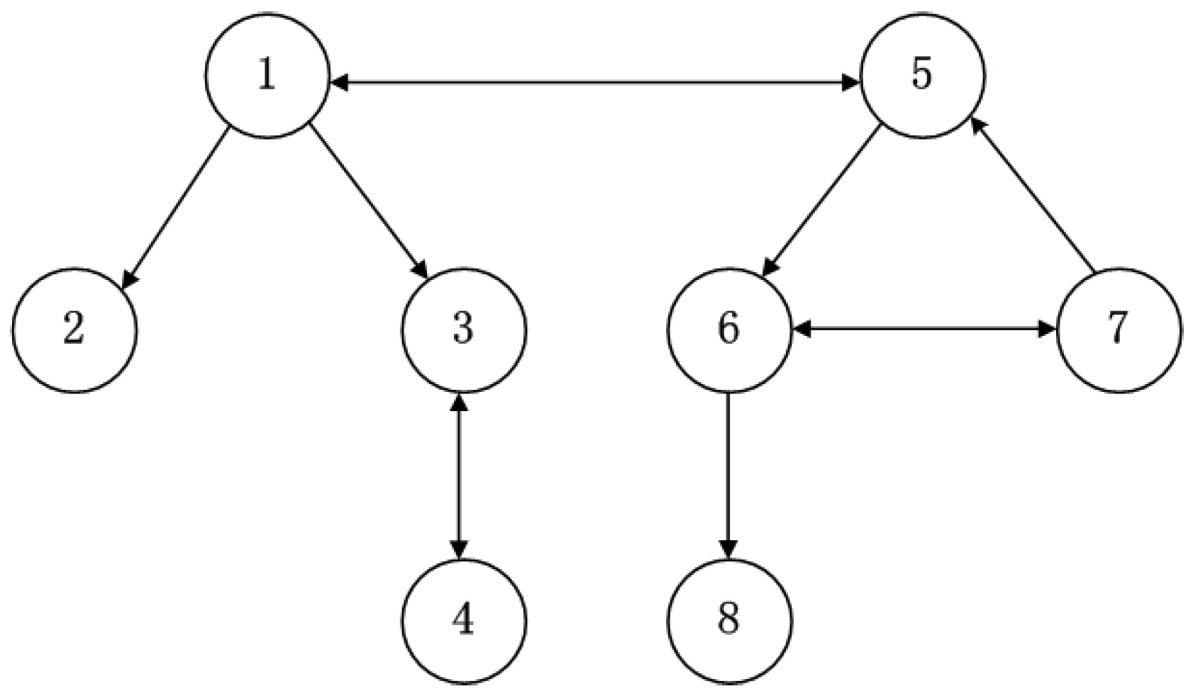
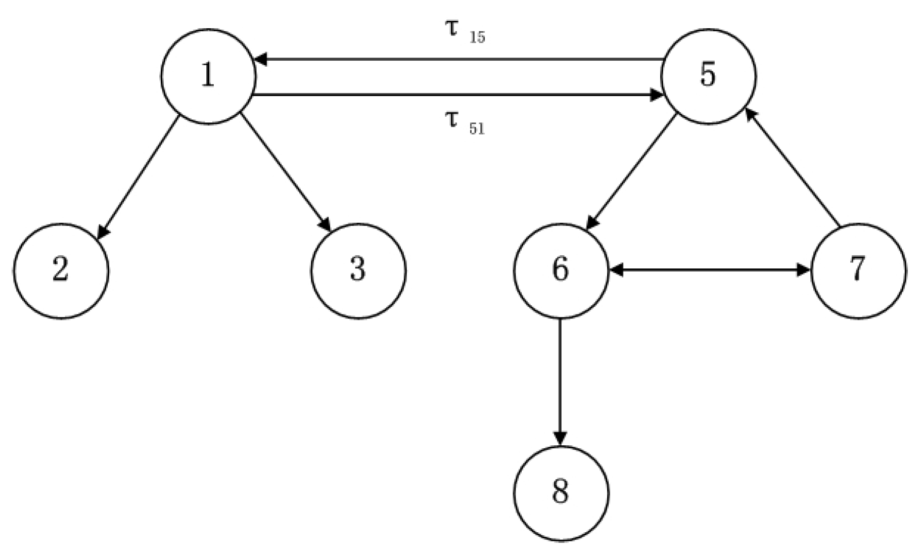
Figure 2 shows the topological structure of two wind farms, where $A_1=\{1,2,3,4\}$ and $A_2=\{5,6,7,8\}$. The value of the output active power is $P_{sA}=40$ MW, and we assume that the key parameters of each unit are those shown in

Table 1. Key parameters of wind turbines in $A_1$.

Parameters	No. 1 WT	No. 2 WT	No. 3 WT	No. 4 WT
$H_{tot}$ (s)	3	5	4	3
$L_m$ (pu)	2.9	2.5	2.8	2.9
$L_s$ (pu)	0.171	0.159	0.181	0.165
$L_r$ (pu)	0.156	0.126	0.149	0.156
$R_r$ (pu)	0.005	0.005	0.004	0.006
$i_{qs}$ (pu)	1.8	1.6	1.5	1.7
$i_{ds}$ (pu)	1.7	1.8	1.6	1.3
$P_e$ (MW)	6.5	7	7.5	6.5

and

Table 2. Key parameters of wind turbines in $A_2$.

Parameters	No. 5 WT	No. 6 WT	No. 7 WT	No. 8 WT
$H_{tot}$ (s)	4	3	5	6
$L_m$ (pu)	2.6	3.0	2.8	2.7
$L_s$ (pu)	0.167	0.172	0.158	0.156
$L_r$ (pu)	0.148	0.151	0.146	0.147
$R_r$ (pu)	0.005	0.008	0.008	0.005
$i_{qs}$ (pu)	1.8	1.9	1.5	1.8
$i_{ds}$ (pu)	1.6	1.7	1.5	1.5
$P_e$ (MW)	6	6	5	5.5

, where WT is the abbreviation of wind turbine.

According to Equation (13), we can take the target value as $T=\left[\begin{array}{c}14\\ 12.6\end{array}\right]$. The initial values are set as $T=T_{10}+T_{20}=\left[\begin{array}{c}5\\ 4.6\end{array}\right]+\left[\begin{array}{c}9\\ 8\end{array}\right]$. On the basis of the complementary control strategy, Equation (19), we have

$$\begin{array}{c}\hfill \left\{\begin{array}{ccc}\hfill {\mu }_1& \hfill =& -y_1-y_5+T+{\overline{\mu }}_1\hfill \\ \hfill {\mu }_2& \hfill =& y_1-y_2+{\overline{\mu }}_2\hfill \\ \hfill {\mu }_3& \hfill =& y_1+y_4-2y_3+{\overline{\mu }}_3\hfill \\ \hfill {\mu }_4& \hfill =& y_3-y_4+{\overline{\mu }}_4\hfill \\ \hfill {\mu }_5& \hfill =& y_7-y_1-2y_5+T+{\overline{\mu }}_5\hfill \\ \hfill {\mu }_6& \hfill =& y_7+y_5-2y_6+{\overline{\mu }}_6\hfill \\ \hfill {\mu }_7& \hfill =& y_6-y_7+{\overline{\mu }}_7\hfill \\ \hfill {\mu }_8& \hfill =& y_6-y_8+{\overline{\mu }}_8\hfill \end{array}\right.\end{array}$$

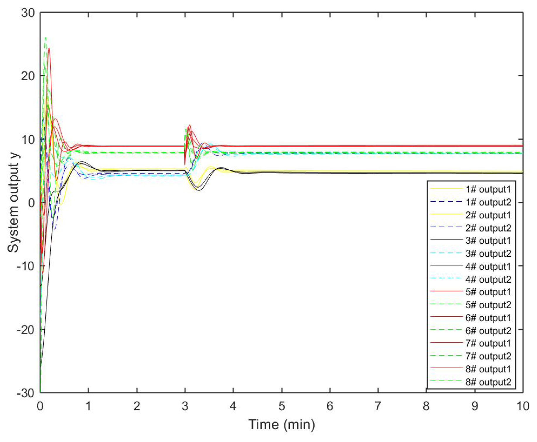
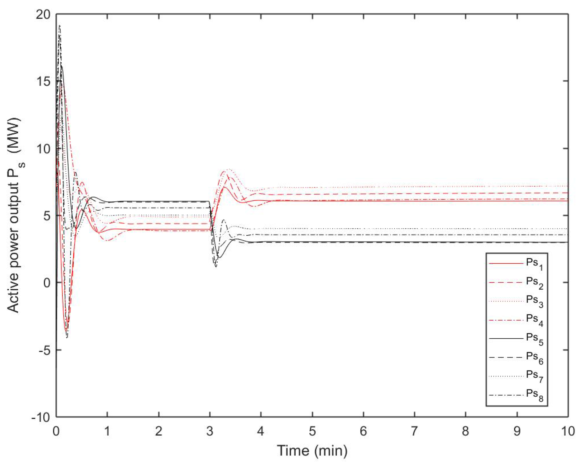
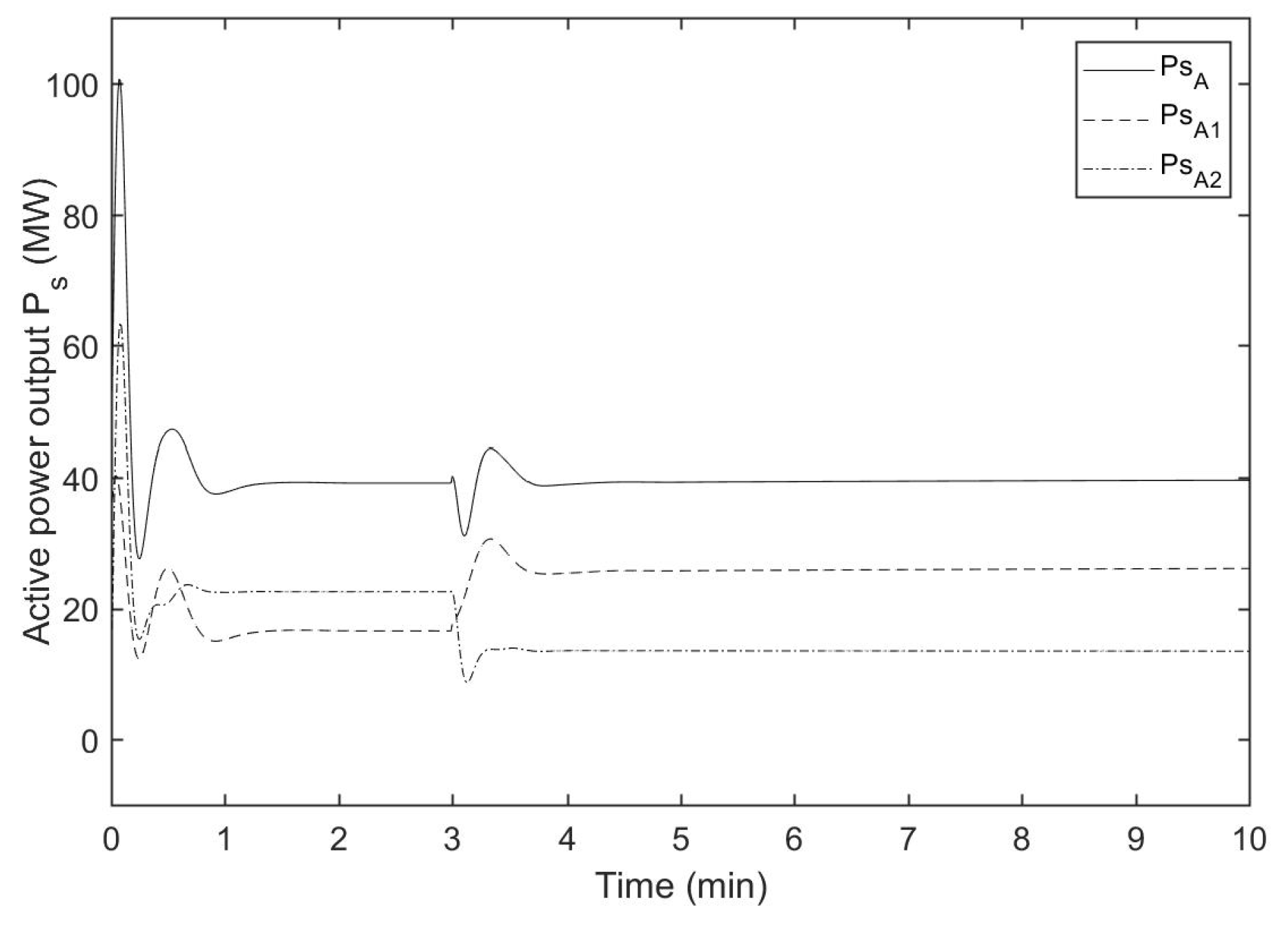
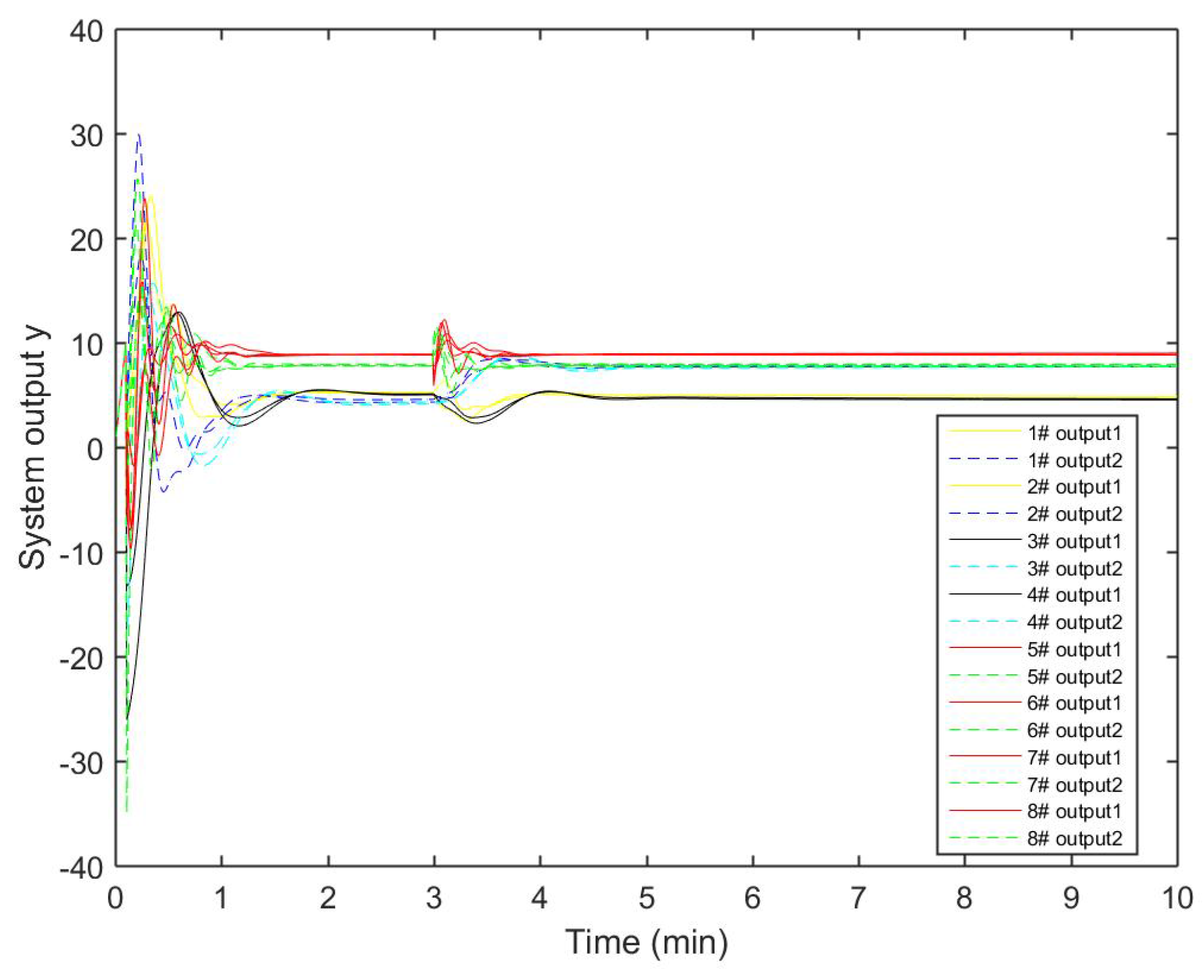
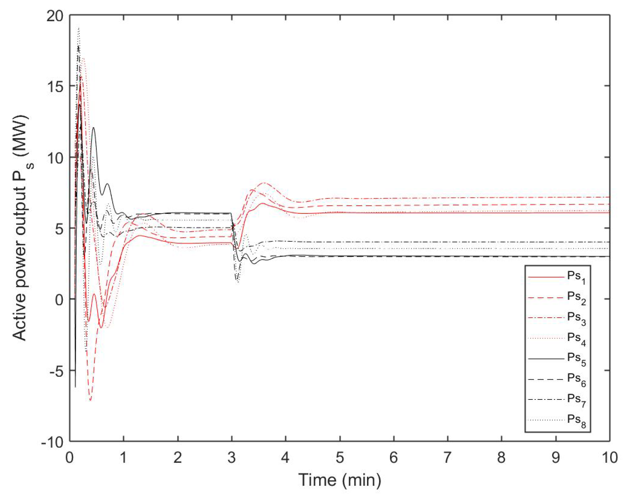
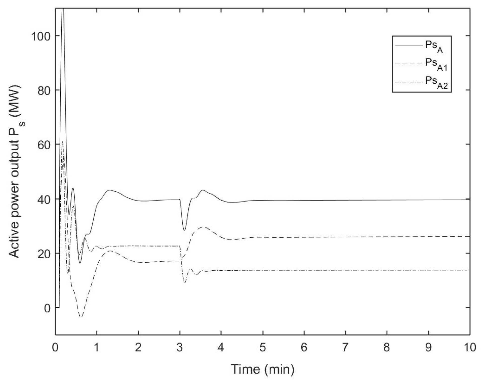
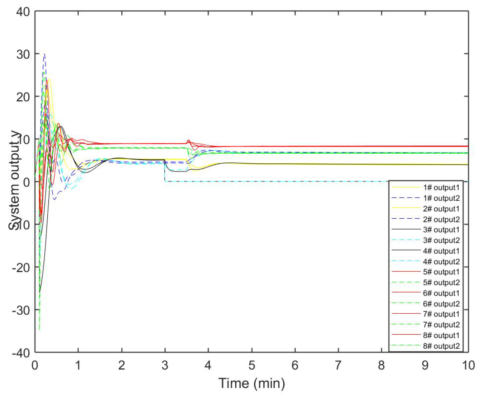
Assuming that, at 3 s, the output $y_k$ and the active power $P_{sk}$ ($k\in A_2$) of the wind turbines in wind farm $A_2$ vary with the wind speed, the response curves are those shown in Figure 3, Figure 4 and Figure 5. Figure 3 shows the system outputs of every wind turbine, Figure 4 shows the active power outputs of every wind turbine, and Figure 5 shows the sums of the active power outputs of the wind farms. Before the 3 s, the wind turbines in the two wind farms are in steady state and the sum of the active power outputs of the two wind farms is 40 MW. Assuming that at 3 s the wind speed is reduced in wind farm $A_2$, the power outputs of wind turbines 5, 6, 7 and 8 are reduced to 3, 3, 4, and 3.5 MW, respectively. According to the complementary control strategy, the active output of each unit in wind farm $A_1$ is regulated as long as there is enough wind energy. The power outputs of wind turbines 1, 2, 3 and 4 are adjusted to 6.1, 6.7, 7.5 and 6.2 MW, respectively. Through the automatic regulation, the total active output of the two wind farms can be maintained at 40 MW.

Figure 3 shows that for $y_j$ ($j\in A_1$), all turbines converge to the same value $y_{A_1}$, and for $y_k$ ($k\in A_2$), all turbines converge to $y_{A_2}$, which means that $y_1=y_2=y_3=y_4=y_{A_1}$, $y_5=y_6=y_7=y_8=y_{A_2}$, and both wind farms achieve output synchronization. In Figure 4 and Figure 5, from 0 to 3 s, the sum of all $P_{si}$ ($i=1,\dots ,8$) can converge to $P_{sA}=40$ MW, which means that $P_{sA}=P_{s{A}_1}+P_{s{A}_2}={\sum }_{j\in A_1}{P}_{sj}+{\sum }_{k\in A_2}{P}_{sk}=40$ MW. At 3 s, because of the reduction in the wind speed, the active power output of every wind turbine in $A_2$ drops. Consequently, $y_{A_1}$ and $P_{s{A}_1}$ are adjusted on the basis of the complementary control. Finally, the total sum of the two wind farms remains unchanged. Therefore, the complementary control target of the active power in the two wind farms is achieved.

5.2. Results of the Complementary Control Considering the Time Delay

Figure 6 shows the topological structure of the wind farms with the communication delay, where $A_1=\{1,2,3,4\}$ and $A_2=\{5,6,7,8\}$. We suppose that a time delay, ${\tau }_{15}$ or ${\tau }_{51}$, exists between the two wind farms. Usually the wind farms are interconnected by the same communication line, and hence, we can take ${\tau }_{15}={\tau }_{51}=0.1$ s. In this subsection, the total power is still $P_{sA}=40$ MW. The key parameters and the initial values are the same as those aforementioned. According to the complementary control strategy given in Equation (26), we have

$$\begin{array}{c}\hfill \left\{\begin{array}{ccc}\hfill {\mu }_1& \hfill =& -y_1\left(t\right)-y_5(t-{\tau }_{15})+T+{\overline{\mu }}_1\hfill \\ \hfill {\mu }_2& \hfill =& y_1\left(t\right)-y_2\left(t\right)+{\overline{\mu }}_2\hfill \\ \hfill {\mu }_3& \hfill =& y_1\left(t\right)+y_4\left(t\right)-2y_3\left(t\right)+{\overline{\mu }}_3\hfill \\ \hfill {\mu }_4& \hfill =& y_3\left(t\right)-y_4\left(t\right)+{\overline{\mu }}_4\hfill \\ \hfill {\mu }_5& \hfill =& y_7\left(t\right)-2y_5\left(t\right)-y_1(t-{\tau }_{51})+T+{\overline{\mu }}_5\hfill \\ \hfill {\mu }_6& \hfill =& y_7\left(t\right)+y_5\left(t\right)-2y_6\left(t\right)+{\overline{\mu }}_6\hfill \\ \hfill {\mu }_7& \hfill =& y_6\left(t\right)-y_7\left(t\right)+{\overline{\mu }}_7\hfill \\ \hfill {\mu }_8& \hfill =& y_6\left(t\right)-y_8\left(t\right)+{\overline{\mu }}_8\hfill \end{array}\right.\end{array}$$

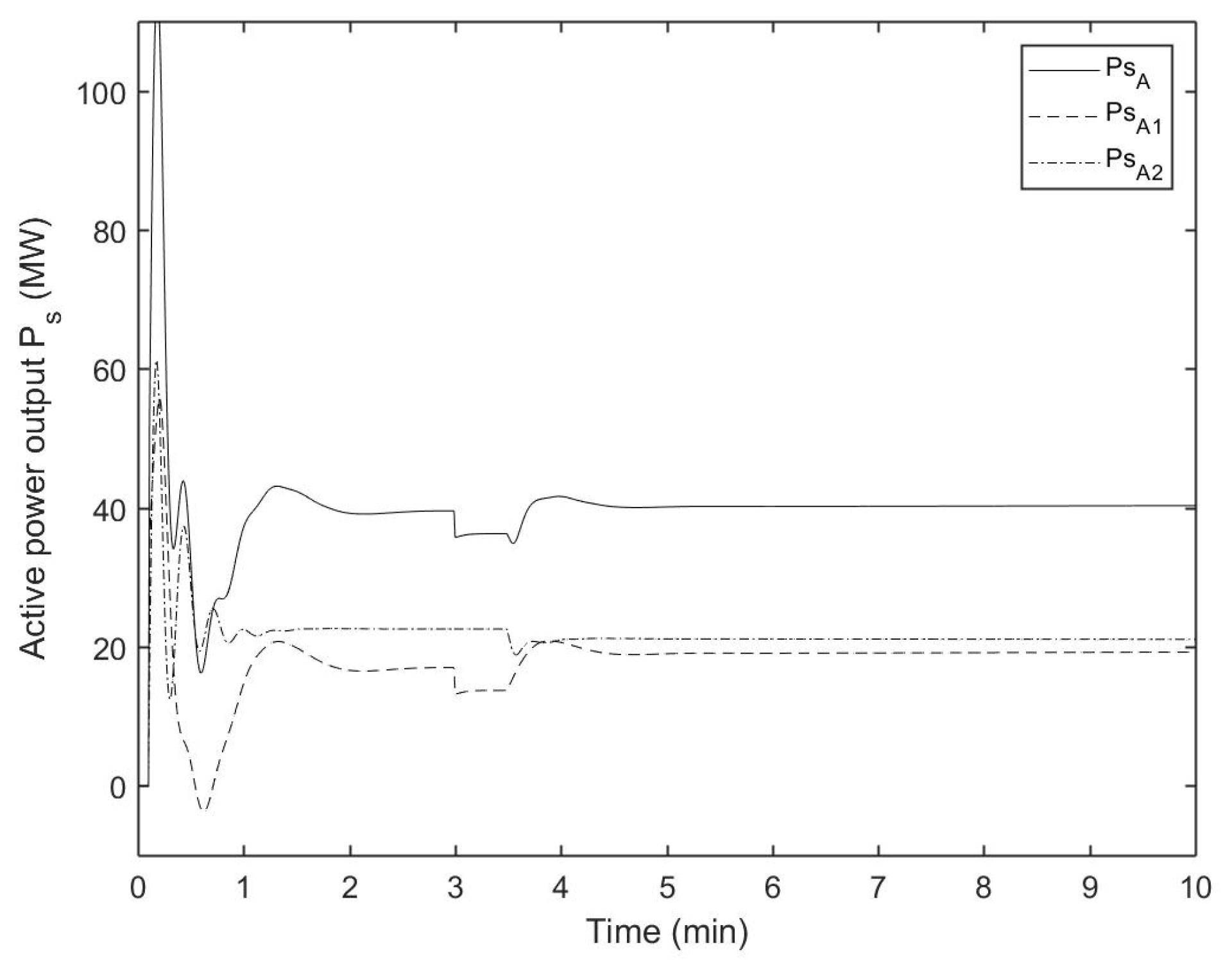
We assume that at 3 s, the output $y_k$ and the power $P_{sk}$ ($k\in A_2$) in wind farm $A_2$ are affected by the wind speed; the response curves are shown in Figure 7, Figure 8 and Figure 9. Figure 7 shows the system outputs of every wind turbine, Figure 8 shows the active power outputs of every wind turbine, and Figure 9 shows the sums of the active power outputs of the wind farms.

It is seen from Figure 7 that the wind turbines in the two wind farms achieve output synchronization, and the outputs $y_{i1}$ and $y_{i2}$ ($i=1,\dots ,8$) can converge to the respective value. In Figure 8 and Figure 9, from 0 to 3s, the sums of $P_{s{A}_1}$ and $P_{s{A}_2}$ can converge to $P_{sA}$ (40 MW). At 3 s, because of the variation in the wind speed, $y_{A_1}$ changes and $P_{sA}$ drops. Then, $y_{A_2}$ and $P_{s{A}_2}$ are adjusted on the basis of the complementary control when a time delay exists. Hence, the sum of all $P_{si}$ can return to $P_{sA}=40$ MW. Therefore, the complementary control target of the two wind farms is achieved when a time delay exists.

5.3. The Results of the Complementary Control after Failure

In this subsection, the failure case is considered. We assume that a failure occurs in wind turbine 4 in $A_1$ at 3 s and that it cannot work thereafter. At 3.5 s, the failure unit is cut off from the network. Figure 10 shows the network topology after the malfunction, and Figure 11, Figure 12 and Figure 13 show the response curves of the outputs.

The simulations show that the whole process can be divided into three stages:

(1) Prior to 3 s, the two wind farms achieve output synchronization, and $y_j$ ($j\in A_1$) and $y_k$ ($k\in A_2$) converge to $y_{A_1}$ and $y_{A_2}$, respectively. The sum of all $P_{si}$ ($i=1,\dots ,8$) converges to the set value $P_{sA}=40$ MW.

(2) At 3 s, wind turbine 4 breaks up, and its output power falls to zero. Between 3 and 3.5 s, the broken machine is still connected to the network. Wind turbine 3 is affected by the failure and falls out of synchronization.

(3) After 3.5 s, wind turbine 4 is cut off. Figure 10 shows that the number of units in the two wind farms is different. Hence, the complementary control strategy needs to be adjusted. According to Equation (25), we have $T^{{}^{\prime }}=\left[\begin{array}{c}8\\ -8.4\end{array}\right]$. Subsequently, the new complementary control is adjusted as

$$\begin{array}{c}\hfill \left\{\begin{array}{ccc}\hfill {\mu }_1& \hfill =& -y_1\left(t\right)-y_5(t-{\tau }_{15})+T^{{}^{\prime }}+{\overline{\mu }}_1\hfill \\ \hfill {\mu }_2& \hfill =& y_1\left(t\right)-y_2\left(t\right)+{\overline{\mu }}_2\hfill \\ \hfill {\mu }_3& \hfill =& y_1\left(t\right)-y_3\left(t\right)+{\overline{\mu }}_3\hfill \\ \hfill {\mu }_5& \hfill =& y_7\left(t\right)-y_1(t-{\tau }_{51})-2y_5\left(t\right)+T^{{}^{\prime }}+{\overline{\mu }}_5\hfill \\ \hfill {\mu }_6& \hfill =& y_7\left(t\right)+y_5\left(t\right)-2y_6\left(t\right)+{\overline{\mu }}_6\hfill \\ \hfill {\mu }_7& \hfill =& y_6\left(t\right)-y_7\left(t\right)+{\overline{\mu }}_7\hfill \\ \hfill {\mu }_8& \hfill =& y_6\left(t\right)-y_8\left(t\right)+{\overline{\mu }}_8\hfill \end{array}\right.\end{array}$$

On the basis of the proposed control strategy, Figure 11 shows that the two wind farms can still obtain a synchronous output. Figure 12 and Figure 13 show that the total active power of the two wind farms can still converge to the set value. Thus, when a single unit fails, the output active power of two wind farms can be complementary to each other by using the complementary control strategy.

The above simulations show that the complementary control strategy with communication delay can achieve the complementary control target for individual output synchronization and overall output complementation. Moreover, the distributed complementary control strategy can effectively reduce the loss caused by fault. Even if a single unit fails, the whole wind farm can still run normally. Therefore, for the complex and changeable environment of offshore wind farms, distributed complementary control can greatly increase the reliability and autonomy of wind farms.

6. Conclusions

On the basis of the Hamiltonian energy method, a distributed control strategy has been proposed to solve the complementary control problem of wind turbines in two offshore wind farms. This control strategy helps the two farms to achieve internal output synchronization and output complementarity between them. In this study, the topological structure of the two offshore wind farms has been considered as a distributed network. First, the distributed complementary control strategy has been developed to achieve the control target of individual output synchronization and overall output complementation, improving the reliability of the offshore wind farms. Second, the energy-shaping method and the newly developed Hamiltonian energy theory for controlling distributed Hamiltonian systems have been applied to the modeling and control of wind turbines. In addition, considering that the two offshore wind farms are far away from each other, the communication delay between them is non-negligible. Therefore, a modified distributed complementary control strategy has been developed to ensure the feasibility of the control strategy in the case of time delay. Finally, the effectiveness of the proposed control strategies has been demonstrated via numerical simulations under three different scenarios. In future work, the distributed complementary control strategy can be further expanded and used for multiple wind farms or wind farm clusters.

References

- Liu, T.Y.; Tavner, P.J.; Feng, Y.; Qiu, Y.N. Review of recent offshore wind power development in China. Wind Energy 2013, 16, 786–803. [Google Scholar] [CrossRef]
- Hou, P.; Hu, W.; Soltani, M.; Chen, Z. Optimized placement of wind turbines in large-scale offshore wind farm using particles swarm optimization algorithm. IEEE Trans. Sustain. Energy 2015, 6, 1272–1282. [Google Scholar] [CrossRef]
- Li, C.H.; Zhan, P.; Wen, J.Y.; Yao, M.Q.; Li, N.H.; Lee, W. Offshore wind farm integration and frequency support control utilizing hybrid multiterminal HVDC transmission. IEEE Trans. Ind. Appl. 2014, 50, 2788–2797. [Google Scholar] [CrossRef]
- Shiau, T.; Chuen-Yu, J. Developing an indicator system for measuring the social sustainability of offshore wind power farms. Sustainability 2016, 8, 470. [Google Scholar] [CrossRef]
- Madariaga, A.; Martin, J.L.; Zamora, I.; Martinez de Alegria, I.; Ceballos, S. Technological trends in electric topologies for offshore wind power plants. Renew. Sustain. Energy Rev. 2013, 24, 32–44. [Google Scholar] [CrossRef]
- Bakka, T.; Karimi, H.R.; Christiansen, S. Linear parameter-varying modelling and control of an offshore wind turbine with constrained information. IET Control Theory Appl. 2014, 8, 22–29. [Google Scholar] [CrossRef]
- Chen, Y.Y.; Dong, Z.Y.; Meng, K.; Luo, F.J.; Xu, Z.; Wong, K.P. Collector system layout optimization framework for large-scale offshore wind farms. IEEE Trans. Sustain. Energy 2016, 7, 1398–1407. [Google Scholar] [CrossRef]
- Khalid, M.; Savkin, A.V. A model predictive control approach to the problem of wind power smoothing with controlled battery storage. Renew. Energy 2010, 35, 1520–1526. [Google Scholar] [CrossRef]
- Zhang, Z.; Xu, H.; Zou, J.; Zheng, G. Sliding mode control-based active power control for wind farm with variable speed wind generation system. Proc. Inst. Mech. Eng. Part C J. Mech. Eng. Sci. 2013, 227, 449–458. [Google Scholar] [CrossRef]
- Prieto-Araujo, E.; Junyent-Ferre, A.; Lavernia-Ferrer, D.; Gomis-Bellmunt, O. Decentralized control of a nine-phase permanent magnet generator for offshore wind turbines. IEEE Trans. Energy Convers. 2015, 30, 1103–1112. [Google Scholar] [CrossRef]
- Wang, B.; Wu, Q.X.; Tian, M.; Hu, Q.Y. Distributed coordinated control of offshore doubly fed wind turbine groups based on the Hamiltonian energy method. Sustainability 2017, 9, 1448. [Google Scholar] [CrossRef]
- Baros, S.; Llic, M.D. A consensus approach to real-time distributed control of energy storage systems in wind farms. IEEE Trans. Smart Grid 2017. [Google Scholar] [CrossRef]
- Wang, L.; Wen, J.; Cai, M.; Zhang, Y. Distributed optimization control schemes applied on offshore wind farm active power regulation. Energy Procedia 2017, 105, 1192–1198. [Google Scholar] [CrossRef]
- Jiang, Q.; Hong, H. Wavelet-based capacity configuration and coordinated control of hybrid energy storage system for smoothing out wind power fluctuations. IEEE Trans. Power Syst. 2013, 28, 1363–1372. [Google Scholar] [CrossRef]
- Li, Y.; Xu, Z.; Østergaard, J.; Hill, D.J. Coordinated Control Strategies for Offshore Wind Farm Integration via VSC-HVDC for System Frequency Support. IEEE Trans. Energy Convers. 2017, 32, 843–856. [Google Scholar] [CrossRef]
- Sakamuri, J.N.; Altin, M.; Hansen, A.D.; Cutululis, N.A. Coordinated frequency control from offshore wind power plants connected to multi terminal DC system considering wind speed variation. IET Renew. Power Gener. 2017, 11, 1226–1236. [Google Scholar]
- Van der Schaft, A.J. L2-Gain and Passivity Techniques in Nonlinear Control; Springer: London, UK, 2000. [Google Scholar]
- Wang, Y.; Cheng, D.; Hong, Y. Stabilization of synchronous generators with Hamiltonian function approach. Int. J. Syst. Sci. 2001, 32, 971–978. [Google Scholar] [CrossRef]
- Xi, Z.; Cheng, D.; Lu, Q.; Mei, S. Nonlinear decentralized controller design for multimachine power systems using Hamiltonian function method. Automatica 2002, 38, 527–534. [Google Scholar] [CrossRef]
- Ortega, R.; van der Schaft, A.J.; Maschke, B.; Escobar, G. Interconnection and damping assignment passivity-based control of port-controlled Hamiltonian systems. Automatica 2002, 38, 585–596. [Google Scholar] [CrossRef]
- Ekanayake, J.B.; Holdsworth, L.; Jenkins, N. Comparison of 5th order and 3rd order machine models for doubly fed induction generator wind turbines. Electr. Power Syst. Res. 2003, 67, 207–215. [Google Scholar] [CrossRef]
- Ledesma, P.; Usaola, J. Doubly fed induction generator model for transient stability analysis. IEEE Trans. Energy Convers. 2005, 20, 388–397. [Google Scholar] [CrossRef]
- Wu, F.; Zhang, X.P.; Ju, P.; Sterling, M.J.H. Decentralized nonlinear control of wind turbine with doubly fed induction generator. IEEE Trans. Power Syst. 2008, 23, 613–621. [Google Scholar]
- Mesbahi, M.; Egerstedt, M. Graph Theoretic Method in Multiagent Networks; Princeton University Press: Princeton, NJ, USA, 2010. [Google Scholar]
- Ren, W.; Beard, R.W. Distributed Consensus in Multi-Vehicle Cooperative Control; Spring-Verlag: London, UK, 2008. [Google Scholar]
- Li, C.S.; Wang, Y.Z. Protocol design for output consensus of port-controlled Hamiltonian multi-agent systems. Acta Autom. Sin. 2014, 40, 415–422. [Google Scholar] [CrossRef]
- Khalil, H.K. Nonlinear Systems, 3rd ed.; Prentice-Hall: Upper Saddle River, NJ, USA, 2002. [Google Scholar]
Figure 1.
Block diagram of the control methodology.
Figure 2.
Topological structure of the two wind farms.
Figure 3.
System outputs of wind turbines in two wind farms.
Figure 4.
Active power outputs of wind turbines in two wind farms.
Figure 5.
Sums of active power outputs of wind farms.
Figure 6.
Topological structure of the two wind farms with communication delay.
Figure 7.
System outputs of wind turbines with communication delay.
Figure 8.
Active power outputs of two wind farms with communication delay.
Figure 9.
Sums of active power outputs of wind farms with communication delay.
Figure 10.
Topological structure of the two wind farms after failure.
Figure 11.
System outputs of wind turbines with communication delay during failure.
Figure 12.
Active power outputs of two wind farms with communication delay during failure.
Figure 13.
Sums of active power outputs of wind farms with communication delay during failure.