Household Energy Expenditures in North Carolina: A Geographically Weighted Regression Approach


Department of Geography, University of North Carolina at Greensboro, Greensboro, NC 27412, USA
*
Author to whom correspondence should be addressed.
†
These authors contributed equally to this work.
Sustainability 2018, 10(5), 1511; https://0-doi-org.brum.beds.ac.uk/10.3390/su10051511
Submission received: 19 April 2018
/
Revised: 6 May 2018
/
Accepted: 8 May 2018
/
Published: 10 May 2018
(This article belongs to the Section Sustainable Urban and Rural Development)
Abstract
:The U.S. household (HH) energy consumption is responsible for approximately 20% of annual global GHG emissions. Identifying the key factors influencing HH energy consumption is a major goal of policy makers to achieve energy sustainability. Although various explanatory factors have been examined, empirical evidence is inconclusive. Most studies are either aspatial in nature or neglect the spatial non-stationarity in data. Our study examines spatial variation of the key factors associated with HH energy expenditures at census tract level by utilizing geographically weighted regression (GWR) for the 14 metropolitan statistical areas (MSAs) in North Carolina (NC). A range of explanatory variables including socioeconomic and demographic characteristics of households, local urban form, housing characteristics, and temperature are analyzed. While GWR model for HH transportation expenditures has a better performance compared to the utility model, the results indicate that the GWR model for both utility and transportation has a slightly better prediction power compared to the traditional ordinary least square (OLS) model. HH median income, median age of householders, urban compactness, and distance from the primary city center explain spatial variability of HH transportation expenditures in the study area. HH median income, median age of householders, and percent of one-unit detached housing are identified as the main influencing factors on HH utility expenditures in the GWR model. This analysis also provides the spatial variability of the relationship between HH energy expenditures and the associated factors suggesting the need for location-specific evaluation and suitable guidelines to reduce the energy consumption.
1. Introduction
Worldwide, energy consumption and its associated greenhouse gas (GHG) emissions has increased over the past few decades [1] and is expected to grow by 28% between 2015 and 2040 [2]. The U.S. households alone are responsible for about 20% of annual global GHG emissions, yet they represent only 4.3% of the global population [3]. High levels of energy consumption take place at the HH level because of electrical appliances, heating and cooling equipment, vehicles, and various goods and services [4]. Electricity, heat, and transportation that are largely dependent on burning fossil fuels are the major sources of greenhouse gas emissions from human activities in the United States [5]. If this trend continues, the Earth’s temperature will rise between 2 and 4.9 degrees Celsius by the end of century [6] resulting in disruptive consequences such as sea level rise [7]. The potential economic cost for the United States is roughly 1.2% of gross domestic product (GDP) for each degree Celsius rise in global temperature with greatest effect in the southeastern part of the country [8]. A better understanding of HH energy expenditure and its key drivers are essential to move forward with more sustainable consumption and reduction of greenhouse gas emissions [9,10].
The influence of various factors such as urban form, socioeconomic, demographic, climate, and housing on energy consumption have been widely studied [11,12,13,14,15,16], yet the empirical evidence is inconclusive [9,17]. The disagreements may exist due to the limitation of datasets, different methodologies, variations in countries, the scale being used, and lack of locational contexts analysis being conducted [18,19]. Most of past energy consumption studies are aspatial in nature neglecting the locational information associated with study areas in the analysis. The importance of understanding the spatial dimension of energy consumption is undeniable [20,21] since local contexts and practices are inherently linked to the energy consumption and sustainability. More differentiated local knowledge (e.g., land-use regulations, policies, and practices) that plays particular role in energy consumption is essential for community-scale urban design [22]. Research addressing spatial aspects thus far has been conducted mostly at the macro scales such as country, region, state or city [1,23,24]. Microscale (e.g., census tract) energy consumption analysis remains under explored [17]. Analytical results drawn from geographically aggregated data are sensitive to the scaler issues such as size of zones (metropolitan statistical area (MSA) versus census tract), which affect the validity and reliability of findings [25]. To minimize this issue, individual level data is recommended. In the absence of such data, however, the smallest geographically aggregated available data is highly preferable [26] especially for policy makers [27].
Conventional ordinary least square (OLS) method utilized in prior studies is incapable of capturing spatial variation of energy consumption in different areas of cities and the location-specific impacts of the driving factors [28]. Tobler’s first law of geography “everything is related to everything else, but near things are more related than distant things” [29] (p. 236) indicates the possible spatial non-stationarity in the geographical data [30]. Therefore, energy consumption in different communities of cities should not be considered as being independent of each other due to spatial autocorrelation [28]. Additionally, the impact of diving factors on energy consumption may vary spatially [28]. Geographically weighted regression (GWR) has been proved to be highly effective in capturing such spatial dimensions, however its potential application in energy consumption has not been utilized [31,32].
This study, thus, seeks to add new understanding to the growing body of literature in identifying the key driving factors for HH energy consumption utilizing geographically weighted regression (GWR) method at the census tracts of 14 metropolitan statistical areas (MSAs) in North Carolina (NC). Our study is different from past studies in at least three ways: First, we use census tract data, the smallest aggregated level data, to examine the relationship between HH energy consumption and various explanatory factors including socioeconomics and demographics, housing characteristics, urban form, and temperature. The utility (electricity and gas) and transportation expenditures are considered as measures of HH energy consumption for our analysis. To our knowledge, no prior study has examined these interactions at finer scale geographic data. Second, we applied geographically weighted regression (GWR) method to capture the spatial variation in HH energy expenditures as well as to identify the spatial factors in energy consumption of different areas of cities. Third, the study area, NC utilized in this analysis has never been examined for energy expenditure context, but warrants attention [33]. The results of this study will provide new understanding about the role of human and spatial context in energy use for planners and policy makers at community level. The paper is organized as follows. Section 2 presents the influencing factors on energy consumption of households and theoretical framework. The modeling methodology is described in Section 3. The results are given in Section 4 followed by a discussion in Section 5. We present conclusions and suggestions for future research in Section 6.
2. Theoretical Framework
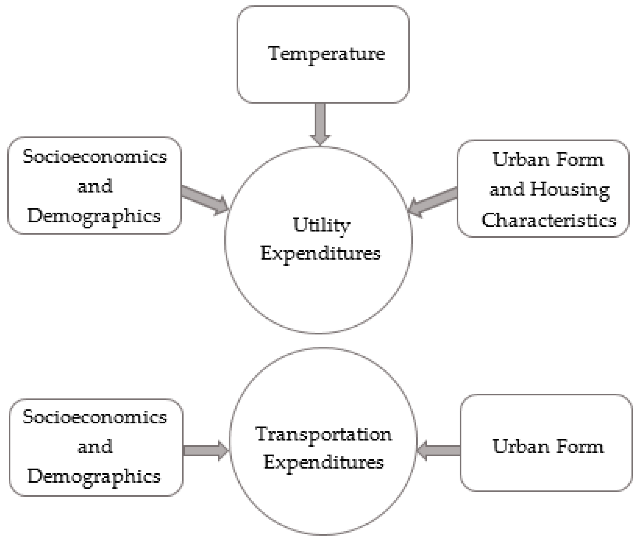
Household (HH) energy consumption has been related to a number of factors including HH characteristics, housing characteristics, urban form, and climate (Figure 1). These factors are reviewed in this section.
2.1. Socioeconomic Characteristics and Demographics
Occupant characteristics have been identified as one of the main factors affecting domestic energy use [11]. Socioeconomic and demographic characteristics of HH such as income, education, size, and age determine households’ social class and their lifestyle [34]. Income is the single largest contributor of HH energy consumption in the U.S. [3]. Higher income groups usually have higher total energy consumption compared to lower income households [35]. Transport and non-transport HH energy use is positively associated with high income in different countries [36,37,38,39]. Education as one of the influencing factors complicates households’ energy use behaviors. On the one hand, higher Educated households tend to adopt more energy efficient technologies and hence have less total energy expenditures [34,40] as well as less transportation related energy consumption [38]. At the same time they may own energy intensive items or commute longer for work [36,41] that will increase their total energy consumption [36,42]. However, Estiri [9] found that socioeconomic status (higher income, education, and better employment status) directly decreases total energy expenditures of U.S. households. The complex relationship between income, education, and energy use behavior may be the result of individuals’ awareness of environmental issues [43].
HH size and age are other significant factors influencing HH energy consumption [11]. A larger number of HH members is associated with higher energy consumption for appliances, larger vehicles, and longer trips [27,41,44,45]. The age of householder is an indication of the life stage [27]. An increase in the age results in higher consumption because the elderly spend more time at home, have a higher income and a higher share of home ownership, and demand higher comfort [43,46]. Older age is also associated with longer non-commuting trips [41,47].
2.2. Urban Form and Housing Characteristics
There is an increasing awareness of the relationship between energy use and urban form/built-environment in existing literature, yet the empirical evidence is inconclusive [17]. Answers vary from cities with higher-density populations consuming lower levels of energy [48] to higher-density populations consuming higher levels of energy [49,50]. Dai et al. [51], however, argue that there are fundamental differences between urban and rural HH expenditure patterns: households living in urban settings with high density and mixed land-uses, and higher connectivity spend less on energy than households living in a geographic setting with lacks in such characteristics. Holden and Norland [52] model residential energy use for heating and travel using a HH survey data of eight areas in Oslo, Norway and suggest compact urban forms can improve energy efficiency and achieve sustainability. Ewing and Rong [16] indicate that an average U.S. HH in compact counties consumes 20% less energy compared to an average HH in low-density leapfrogging development counties. This is mostly due to the higher likelihood of living in a multifamily housing with less floor area in a compact county [16]. In these structures, many surfaces such as walls, floors, and ceilings are shared that may prevent any heat loss or gain.
The significant impact of housing characteristics on energy use has also been identified in the literature. Energy consumption not only increases by size of the house [37], but also based on the type of housing especially for attached or detached units [34]. Living in detached housings results in higher energy consumption due to larger space and more exposed walls [9,16,53,54,55]. Similarly, an increase in the number of rooms in a building results in higher energy used in the building [34,39]. Age of building has been identified as another important factor influencing energy consumption. In recent decades much focus has been targeted on the housing stock for improving energy efficiency of buildings through technologies and policies [9,37,45,56]. Therefore, the modern and new homes are built with more energy efficient features [57]. However, research shows income is the single largest contributor of HH energy consumption [3] and America’s more expensive houses are located in newly built low density suburban areas [58]. With more disposable income, these homeowners may be more frivolous with their energy consumption and long-distance commute.
The opposite seems to be true for older neighborhoods that enjoy the benefit of well-developed infrastructures and are conducive to alternative mode choices such as public transit, walking, and biking [58]. These neighborhoods have less vehicle mile travel (VMT) [41,59], and automobile ownership [60] resulting in less energy consumption [61,62,63]. Though the urban form impacts travel choices and hence energy use, socioeconomic factors are probably more important than built environment characteristics [64]. Despite the significant progress in understanding the relationship between the urban form and energy expenditures, further analysis is needed at microscale for more robust conclusions [17].
2.3. Temperature
The impact of climate change and temperature on residential energy consumption has been well documented [1,27,65,66]. There is a non-linear relationship between temperature and energy use [66,67] as electricity and gas demand increase for both low and high temperatures and decrease for Intermediate temperatures [67]. However, Zhou et al. [68] indicate that the socioeconomic variations in population are of equal or greater importance than climate in the U.S. state-level building energy demand. The mixed results might be due to various climate models, different choices of locations, and spatial and temporal resolutions [68].
2.4. Summary
While the importance of understanding the spatial dimension of energy consumption has been identified [20,21], none of the studies reviewed in Section 2 have examined locational variability of primary drivers of HH energy consumption. Understanding energy consumption of households is a complex issue that requires more comprehensive research at micro-scale with more sophisticated methodology that can capture such spatial variations [18,49,69]. A knowledge gap exists in the use of spatial methods to investigate household energy consumption. Therefore, this study utilizes a geographically weighted regression (GWR) approach to fill this gap.
3. Study Area, Data and Methodology
3.1. Study Area
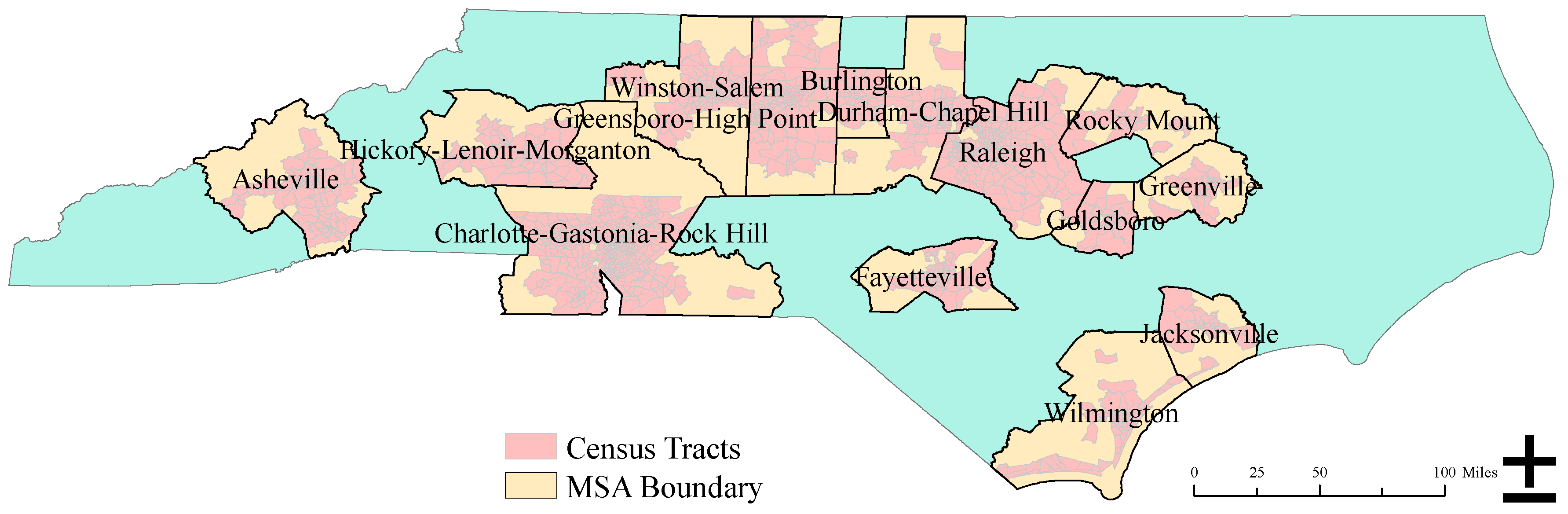
This study uses census tracts of the 14 metropolitan statistical areas (MSAs) in NC (Figure 2). The 2010 MSA boundary is used because sprawl index, which is used as an urban form variable in our analysis, is based on the 2010 census tract boundary. These MSAs include Asheville, Burlington, Charlotte–Gastonia–Rock Hill, Durham–Chapel Hill, Fayetteville, Greensboro–High Point, Goldsboro, Greenville, Hickory–Lenoir–Morganton, Jacksonville, Raleigh–Cary, Rocky Mount, Wilmington, and Winston–Salem. The study area has 1681 tracts, but only 1394 tracts are used for analysis after removing tracts with missing values. The transportation and residential are the largest energy consumption sectors (28.1% and 27.4% of all energy use sectors respectively) in NC [70]. The State’s energy supply is mainly based on petroleum, coal, nuclear power, and natural gas and is depended on imports from other states [71]. NC is one of the fastest growing states [72] and is ranked 13th highest in carbon dioxide emissions in the US in 2010 [33]. A mix of dense and sparse landscapes makes NC a perfect place to study energy issues. Additionally, the researchers’ familiarity with the state provides good working knowledge of the study area.
3.2. Data Collection
A comprehensive consumer survey database from SimplyAnalytics [73]—a web-driven database with supporting data visualization—allows us to understand households’ energy expenditures at census tract geography, the finest geographically scale energy expenditures data available at the time this research is conducted. SimplyAnalytics provides various kinds of data from the top-rated data surveying sites, including: Easy Analytic Software Inc. (EASI), Applied Geographic Solutions (AGS), Mediamark Research (MRI), Dun & Bradstreet (D&B), Nielsen, and Simmons Research [73]. The 2015 average energy expenditures data by households along with census tract geography shapefiles for 14 MSAs of NC are collected from this database. Average HH expenditures are separated into two major groups: utility and transportation and both are given in dollar values. The utility expenditures include households’ average expenditures on both electricity and natural gas for our analysis. Transportation expenditures include vehicle purchase, vehicle leases and rentals, gasoline and oil and other expenses (e.g., maintenance and repair). Expenditure data for census tracts were also added to ArcGIS 10.4 to conduct hot spot analysis. The four factors and their main explanatory variables are presented in Table 1. The socioeconomic and demographic variables including HH median size, householder media age, HH median income, percent of households with education less than high school, and percent of households with bachelor degree are also obtained from SimplyAnalytics. Two housing variables collected from SimplyAnalytics are housing median year and percent of occupied housing with 1 unit detached. Percent of occupied housing units with 4 or more bedrooms is collected from the 2015 American Community Survey (ACS) 5-year estimate data [74].
To evaluate the impact of built environment on households’ energy expenditures, sprawl index at census tract level was collected from National Cancer Institute [75]. The composite metric or sprawl index is developed by combining four multi-dimensional metrics including density, mixed, centering, and street accessibility to capture distinct dimensions of spatial urban form [75]. A set of geographic characteristics (e.g., population density, employment density) is used to calculate each factor. Overall scores are transformed with a mean of 100 and a standard deviation of 25 to create the sprawl index. The higher the number, the more compact the census tract is. The sprawl index is proven to be useful to evaluate travel impacts such as per-capita transportation energy consumption; quality of public transit; and energy efficiency [76]. Therefore, this index is selected for its reliability and validity. Distance from each census tract to the center of primary city of each MSA is used as another variable for assessing the impact of urban form on energy use. The length of the shortest path between each census tract and city center (represented by city hall) within each MSA was measured along the road network by using service area tool of ArcGIS Network Analyst. The road network was developed using 2017 data from North Carolina Department of Transportation (NCDOT) and South Carolina Department of Transportation (SCDOT) [77,78] because both of these organizations make road network data publicly available only for the current year. From our local experience, road network for NC and SC did not change much from 2015 to 2017, so our network distance from each census tract to city center variable should be consistent with our 2015 analysis. Additionally, use of 2017 road network data should not have much influence on the results since we did not focus on specific locations (e.g., homes, facilities). Age of housing is also being used as proxy measure for urban form [17,58,79], as older homes in urban areas are more likely to be in older core areas of cities (near city center) with higher density mix land uses, sidewalks, and interconnected streets networks [80]. Finally, the temperature data for the warmest and coldest months in 2015 for all counties of NC and three counties of SC are collected from Land-Based Station Data of NOAA [81]. ArcGIS 10.4 is used for Kriging interpolation to estimate temperature values across NC. The average temperature values of each census tract are calculated by the mean of raster cells within each census tract using zonal statistics.
3.3. Methodology: ANOVA, Hot Spot Analysis, and GWR
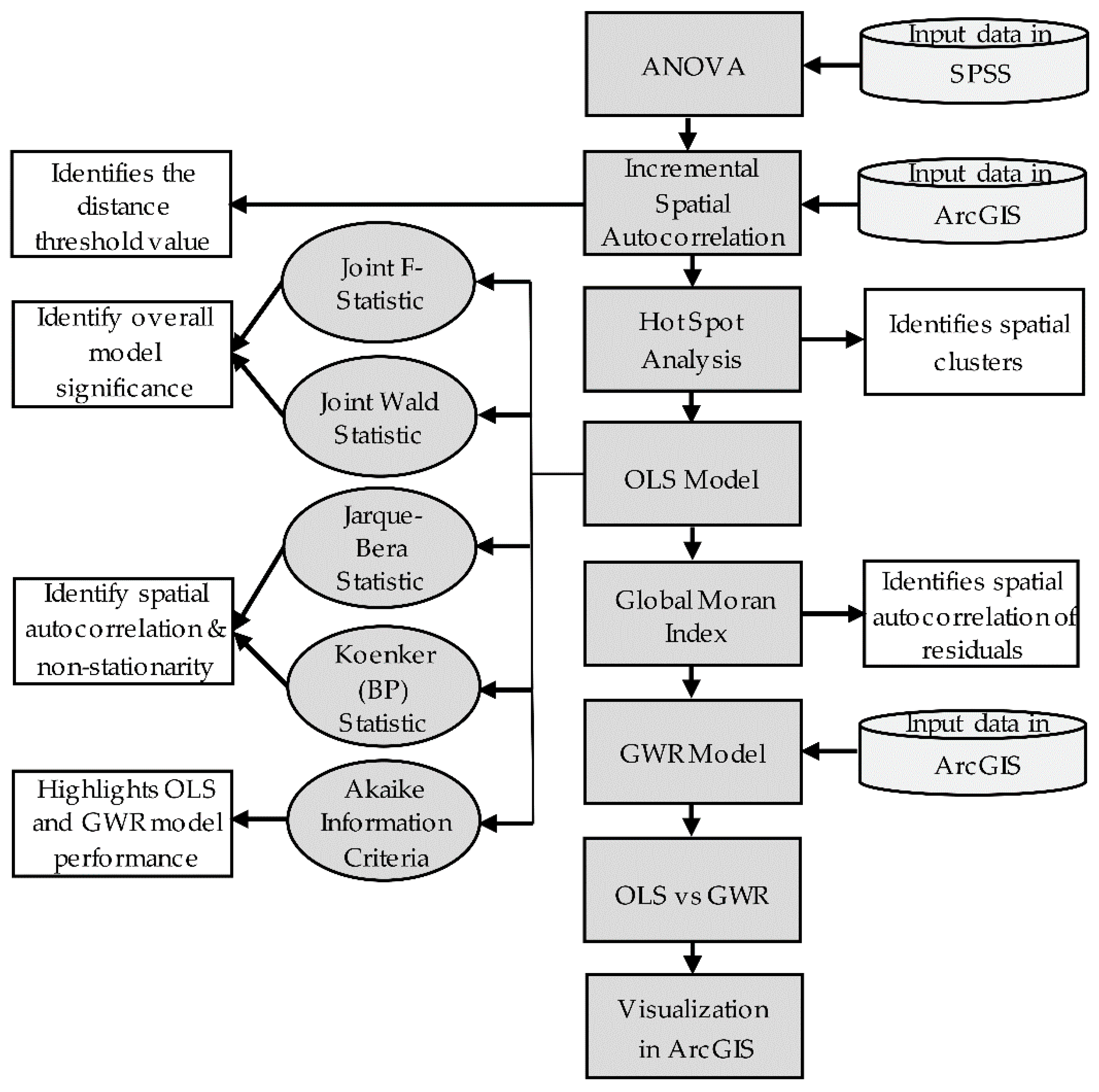
Both spatial and non-spatial analyses are conducted to investigate HH energy expenditures. The methodological procedure is shown in Figure 3. Analysis of variance (ANOVA) is performed using SPSS version 24 to identify whether there is a statistically significant difference in HH energy expenditures among the 14 MSAs. Levene statistic shows that the assumption of homogeneity of variances is violated for both transportation and utility expenditures, therefore Welch ANOVA is utilized. Multiple Comparison table in Games–Howell test is also performed to identify which of the specific groups differ in energy expenditures. The expenditures data for utility and transportation are then added to ArcGIS 10.4 to conduct hot spot analysis. We first perform Incremental Spatial Autocorrelation to identify the appropriate distance threshold values (34,068 m for utility expenditure and 49,294 m for transportation expenditure) for the hot spot analysis [82]. The Hot Spot Analysis (Getis–Ord Gi* statistic) tool is used to calculate the z-score and p-value for each census tract to show where the high or low energy expenditure values cluster. The larger the positive z-score, the more intense the clustering of high values (hot spot), and the smaller the negative z-score, the more intense the clustering of low values (cold spot).
We used geographically weighted regression (GWR) since the OLS method assumes spatial data are stationary and parameter estimations are constant across space [82]. This assumption is hard to meet in many circumstances [31]. Brunsdon et al. [31] developed a geographically weighted regression (GWR) model to account for spatial variations in estimating parameters. GWR extends the OLS model by allowing the coefficients to vary in different locations [31]. We first performed an ordinary regression model to find out the global effects of our explanatory variables on energy expenditures. OLS model also allows us to highlight the performance of the GWR model [31]. Adjusted R-Squared (R2), Akaike Information Criteria (AICc), Joint F and Wald statistics, Jarque–Bera statistic (JB), Koenker (BP) statistic, Variance Inflation Factor (VIF), and Global Moran Index (Moran’s I) are performed in ArcGIS 10.4 to get a properly specified OLS model [82].
Using GWR4 software, we first test the geographical variability of our explanatory variables with the GWR calibrated F-test and Akaike Information Criterion (AICc), where a positive AICc (DIFF of Criterion) suggests no spatial variability in terms of model selection criteria [83]. Therefore, the variable is better to be considered as global rather than local in the model [83]. Two out of seven explanatory variables (percent of households with education less than high school and percent of households with bachelor degree) in transportation model and three out of twelve variables (Sprawl, percent of households with education less than high school and mean January temperature) in utility model showed no spatial variability. Hence, a semiparametric GWR is performed applying an adaptive Gaussian kernel type and the Golden selection search function to select the optimal bandwidth size based on the AICc value [82]. The semiparametric model combines both geographically local and global fixed terms to improve its performance [82]. The adaptive kernel function is selected here due to the various sizes of census tracts [79]. The Gaussian model is selected to ensure there is sufficient local information to calibrate a local regression model [84]. AICc is a useful diagnostic to compare the goodness-of-fit for OLS and GWR models [85]. The overall fit performance and the possible improvements of GWR over OLS model are examined with an analysis of variance (ANOVA) in GWR4 software [86]. The spatial autocorrelation of residuals for both models are finally tested and compared using global Moran’s I in ArcGIS 10.4 [82,87].
4. Results
4.1. Average Household Energy Expenditures in the MSAs
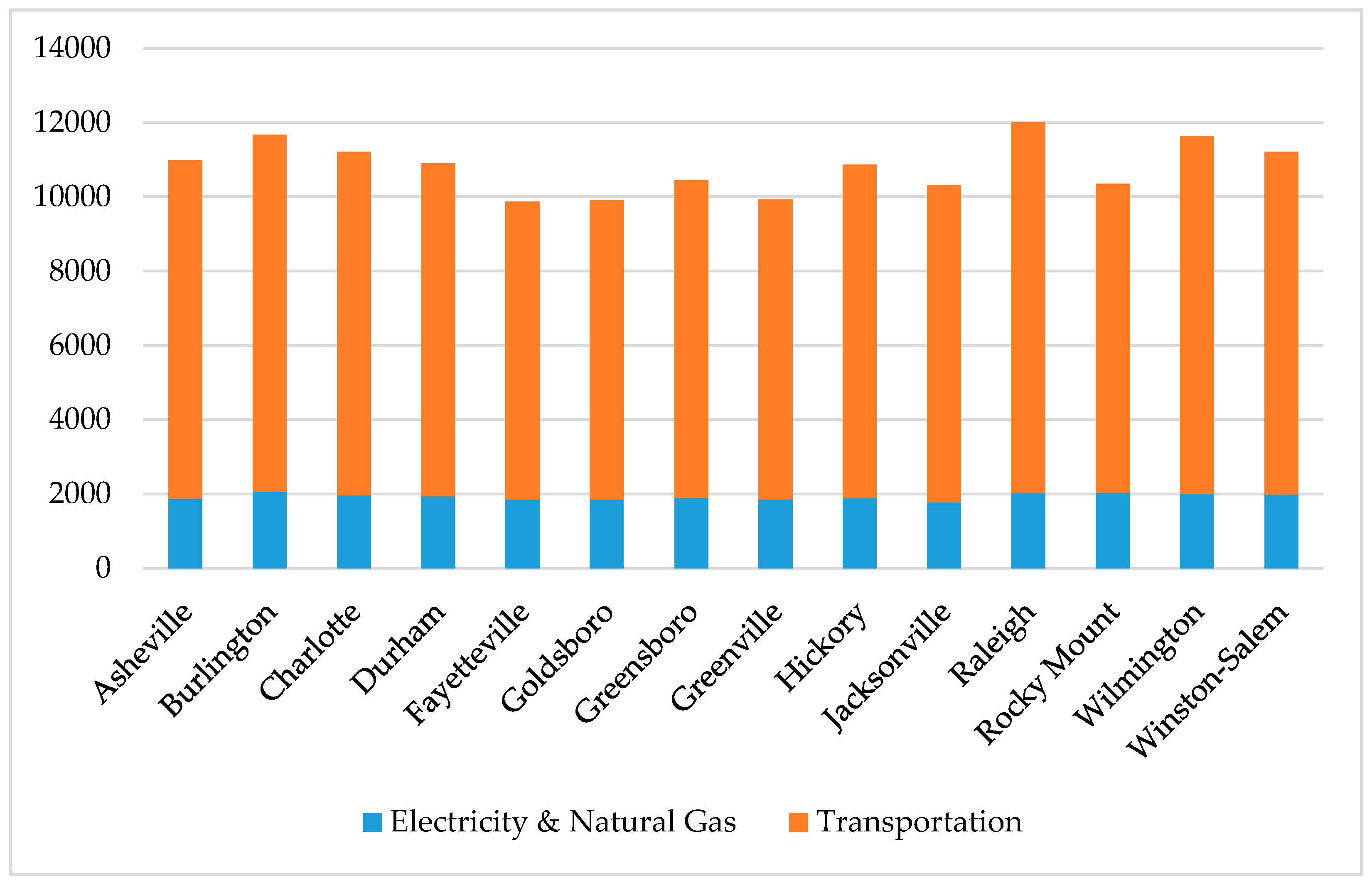
The average HH energy expenditures both in utility (electricity and natural gas) and transportation (excluding public transportation) in NC are nearly $2000 and $9000 per year respectively, which are more like that of U.S. HH average spending [88]. Transportation accounts for almost 80% of HH energy expenditures in all MSAs in NC (Figure 4). The combined average HH energy expenditures of utility and transportation in Raleigh, Burlington, and Asheville MSAs are the highest, while households in Fayetteville, Goldsboro, and Greenville MSAs have the lowest (Figure 4). ANOVA results show significant (p < 0.05) differences in average energy expenditures for both transportation and utility among 14 MSAs. A post hoc Games–Howell test indicates only Raleigh MSA differs significantly from Jacksonville and Fayetteville MSAs in utility expenditures. Fayetteville MSA differs significantly from Asheville, Charlotte–Gastonia–Rock Hill, and Wilmington MSAs in transportation expenditures. Other significant differences (p < 0.05) in transportation expenditures are observed between Wilmington and Greensboro–High Point MSAs; and Raleigh and all other MSAs except Asheville, Burlington, Durham–Chapel Hill, Wilmington, and Winston–Salem.
Nationwide, households spend almost 15% to 19% of their income on transportation [89]. However, only 30% of households in NC falls into this range. Households in our study area spent 4–40% of their income on transportation. We also identified top 10 census tracts with highest and lowest energy expenditures (not shown in table). Most of the census tracts with highest energy expenditures are in Raleigh and Charlotte, the two largest cities in NC. Wake County in Raleigh and Mecklenburg County in Charlotte MSAs are home of some of the wealthiest neighborhoods. However, two census tracts with lowest HH expenditures are also in these two counties. Other census tracts with lowest energy expenditures are located in Durham–Chapel Hill, Greensboro–High Point, and Winston–Salem MSAs.
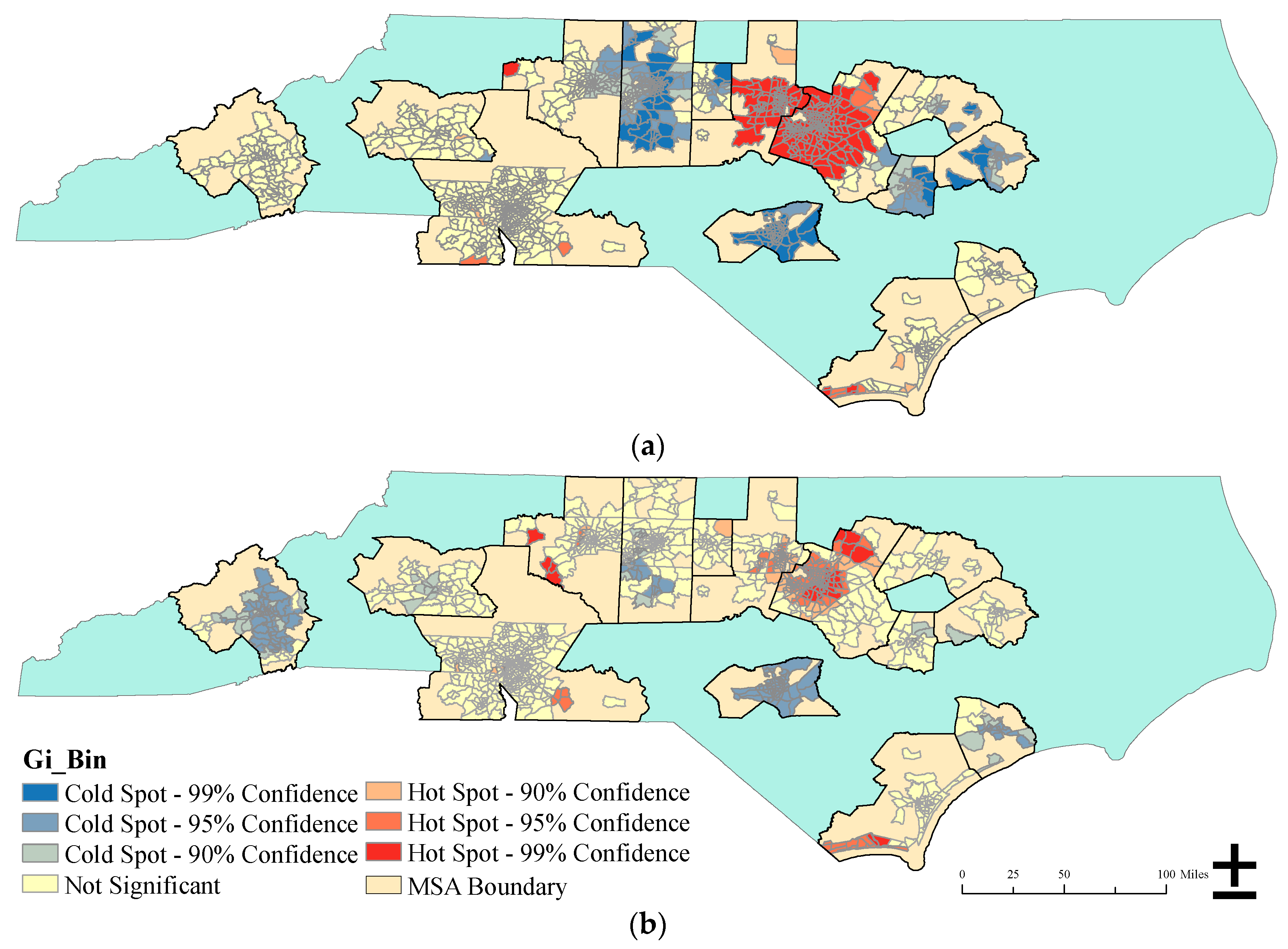
4.2. Hot and Cold Spots
The hot spot analysis shows the cluster of census tracts with high and low energy expenditures (Figure 5). Significant hot spots for HH transportation expenditures are found in Raleigh and Durham–Chapel Hill MSAs (Figure 5a). Significant cold spots for HH transportation expenditures are observed in Greensboro–High Point MSA, eastern parts of Alamance County in Burlington MSA, Fayetteville, Goldsboro, and Greenville MSAs. The significant hot spots for utility expenditures are found in Wake and Franklin counties in Raleigh MSA, areas close to Durham downtown in Durham–Chapel Hill MSA, and Brunswick County in Wilmington MSA (Figure 5b). Significant cold spots for utility expenditure are located in Fayetteville, Jacksonville, and Asheville MSAs.
4.3. OLS Model
The model estimates for transportation and utility are presented in Table 2 and Table 3. The models explain approximately 41% (Adj. R2 = 0.41) variation for transportation (Table 2) and 12% (Adj. R2 = 0.12) variation for utility expenditures (Table 3) in the explanatory variables. The adjusted R2 is a recalibration of the R2 to prevent the artificial increase of R2 when more variables are added in a model [90]. The Joint F-statistic and Joint Wald statistic are used to assess the model significance [90]. The Joint F-statistic is only used when the Koenker (BP) test is not significant [90]. Here, the Koenker (BP) statistic is significant, therefore the Joint Wald statistic shows an overall model significance. In addition, the statistically significant Koenker (BP) test highlights the presence of heteroscedasticity and/or non-stationarity making the transportation and utility models good candidates for GWR analysis [82]. The statistically significant Jarque–Bera statistic indicates that the residuals are not normally distributed [82]. This is additionally confirmed by Moran’s I test.
The transportation OLS model includes all the socioeconomic–demographic and urban form variables listed in Table 1. All of selected variables except HH median size are significant at the 0.01 level (Table 2). HH median income is identified as the most significant variable contributing to the model. With every $100 increase in HH median income in a census tract, there is $3 increase in the HH transport expenditures. Transportation expenditures are also increased with an increase in householder median age and college education. Percent of households with less than high school education in a census tract is associated with lower transportation expenditures. The relationship between both urban form variables and transportation expenditures is statistically significant suggesting that households living in more compact areas and closer to city center of primary city spend less on transportation (Table 2). While all identified variables in Table 1 are entered in the utility model, the low adjusted R2 (0.14) (Table 3) shows that none of the independent variables are strong predictors of utility expenditures. HH median income, HH median age, and percentage of occupied housing with one unit detached are the only significant explanatory variables in the OLS model. Any increase in these variables will increase HH utility expenditures. The VIF values of explanatory variables for both transportation and utility model are less than the critical value of 7.5 indicating that there are no multicollinearity problems between the predictors [82,90].
4.4. OLS Model vs. Semiparametric GWR Model
Significant Moran’s I test (MI = 0.005 p = 0.04) for transportation expenditures highlights the existence of spatial autocorrelation in residuals (Table 2). Although Moran’s I test is not significant for utility expenditures (Table 3), we perform the GWR analysis for both transportation and utility to examine the spatial variability of explanatory variables. The GWR results are shown in Table 4.
A positive DIFF of Criterion in the GWR results, mainly greater than or equal to two, suggests that the local variable is better to be considered as global. The GWR calibrated F-test and the AICc values in the GWR4 software for both transportation and utility confirm that four variables (sprawl, distance from city center, HH median income, householder median age) in transportation model and three variables (percent of housings with one unit detached, HH median income, householder median age) in utility model exhibit statistically significant geographic variability representing by negative DIFF of Criterion and t-values greater than two (p < 0.05) (Table 5). Although there is no change in the signs of the regression coefficients in both the OLS and the semiparametric GWR models, adjusted R2 is one percent better compared to OLS model for both transportation and utility (Table 4). AICc value of the semiparametric GWR decreased by 5.34 and 6.21 in transportation and utility models respectively (Table 4). The simulated residual of the GWR models are also less than that of the global models for transportation and utility. Accordingly, Moran’s I test of GWR model shows a smaller value for transportation (MI = 0.002; p = 0.3) suggesting more random patterns in returned residuals [82] (Table 4). The mean values of the local regression coefficients of explanatory variables for both transportation and utility models have the same signs observed in the OLS models (Table 6). ANOVA tests for transportation (F = 2.67) (Table 7) and utility (F = 2.2) (Table 8) reveal that the predictions improve by applying the semiparametric GWR model.
4.5. GWR Local Estimates
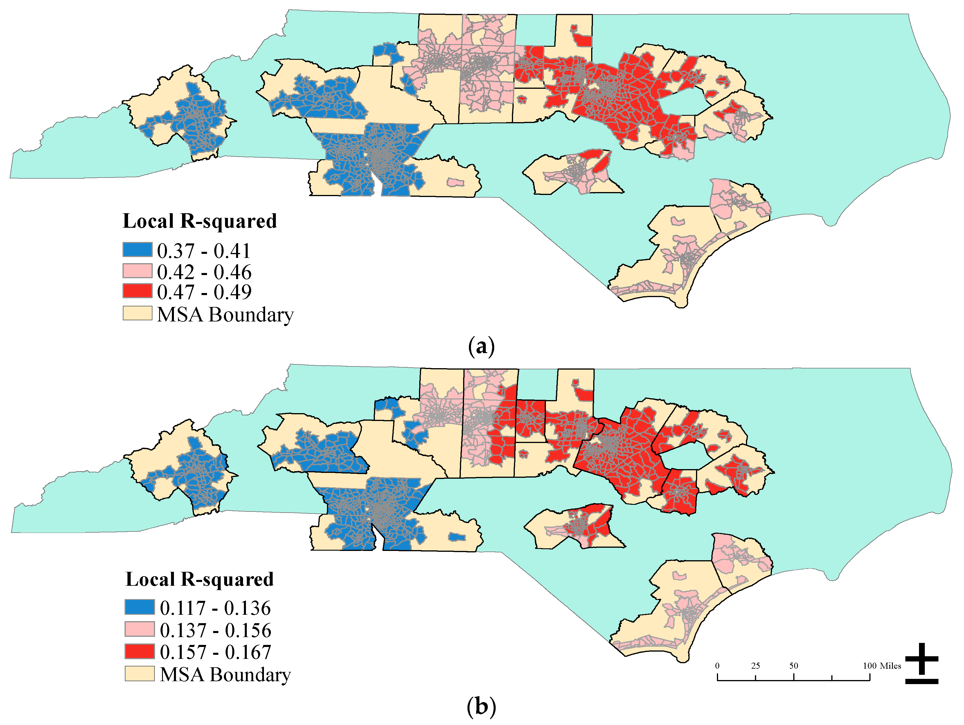
GWR modeling allows for visualizing the spatial patterns of explanatory variables and the goodness of fit [84]. The local estimated coefficients and the local R2s are mapped and shown in Figure 6. The t-values are mapped only when the variables’ coefficients are not significant (t < 2) in some parts of the study area. The local goodness of fit shows spatial differentiation, with values from 0.37 to 0.49 for transportation and 0.12 to 0.17 for utility (Figure 6). Higher values are observed in the east part of study area for both models reflecting that GWR can successfully characterize spatial non-stationarity [82].
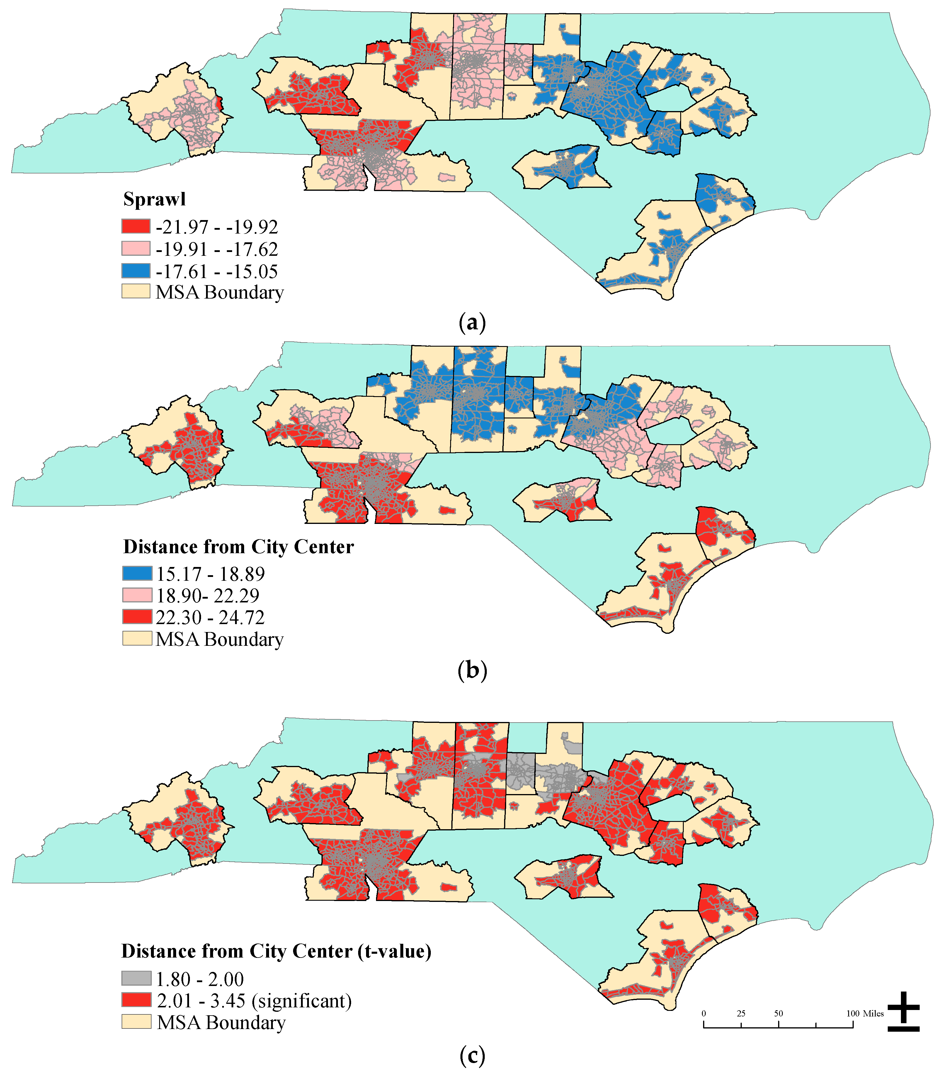
Sprawl local estimates have a higher significant influence on transportation expenditures in the west part of study area particularly in Winston–Salem, Hickory–Lenoir–Morganton, and northern part of Charlotte MSAs suggesting that with every increase in the sprawl score (higher compactness), transportation expenditures decrease in larger values ($19.92–$21.97) compared to the rest of the study area (Figure 7a). Distance from city center has the highest effect on transportation expenditures in Hickory–Lenoir–Morganton, Charlotte–Gastonia–Rock Hill, Asheville, Fayetteville, and Wilmington MSAs. The lowest influence of this variable is observed in Winston–Salem, Greensboro–High Point, and west of Raleigh MSAs (Figure 7b).
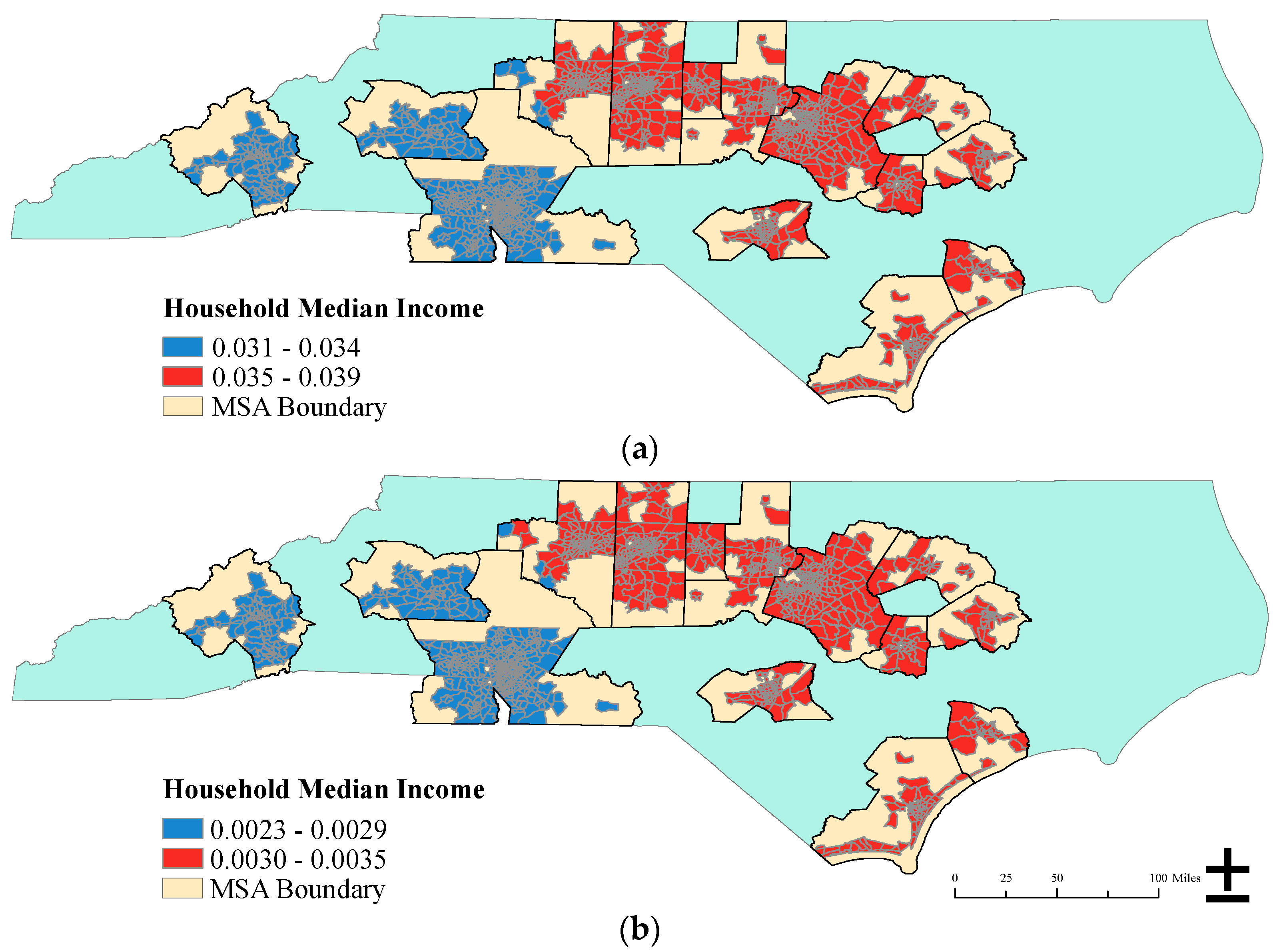
Although there is not a large difference among the local estimates of HH median income, an east–west pattern can be seen for the positive impact of HH median income on both transportation and utility expenditures (Figure 8).
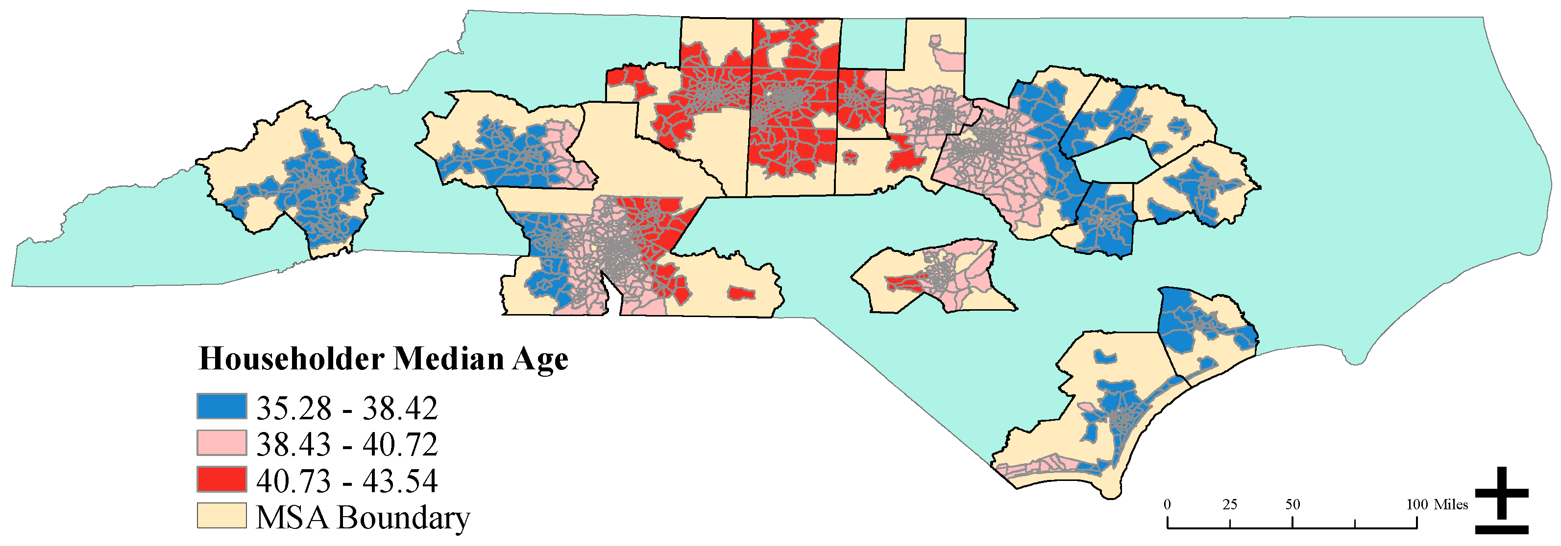
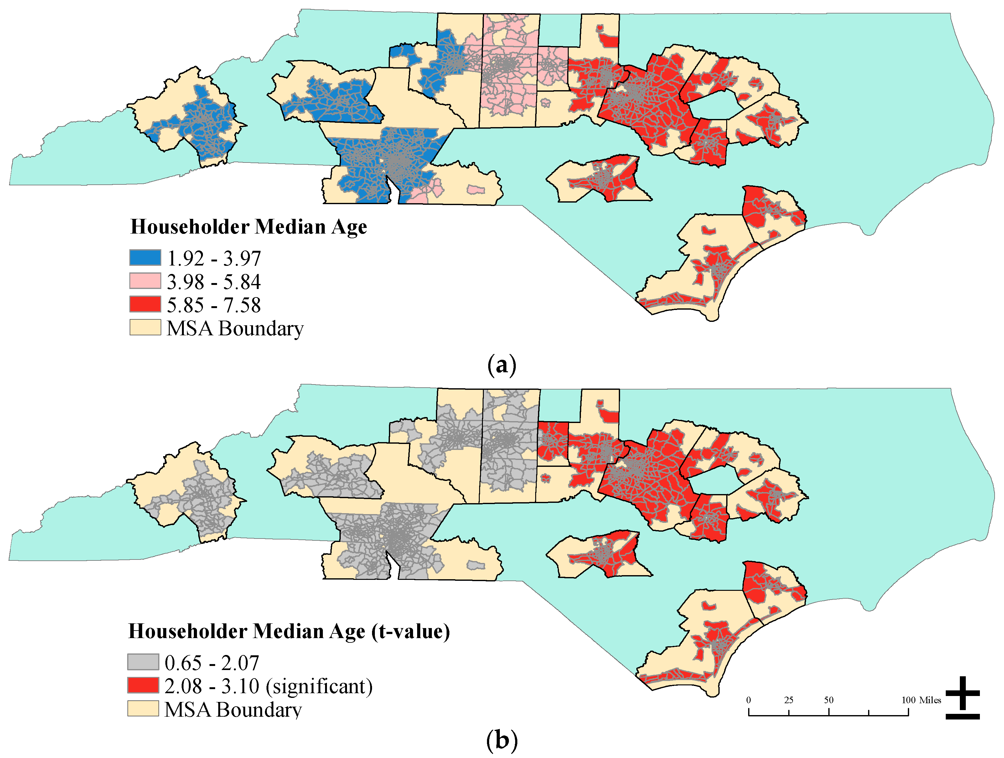
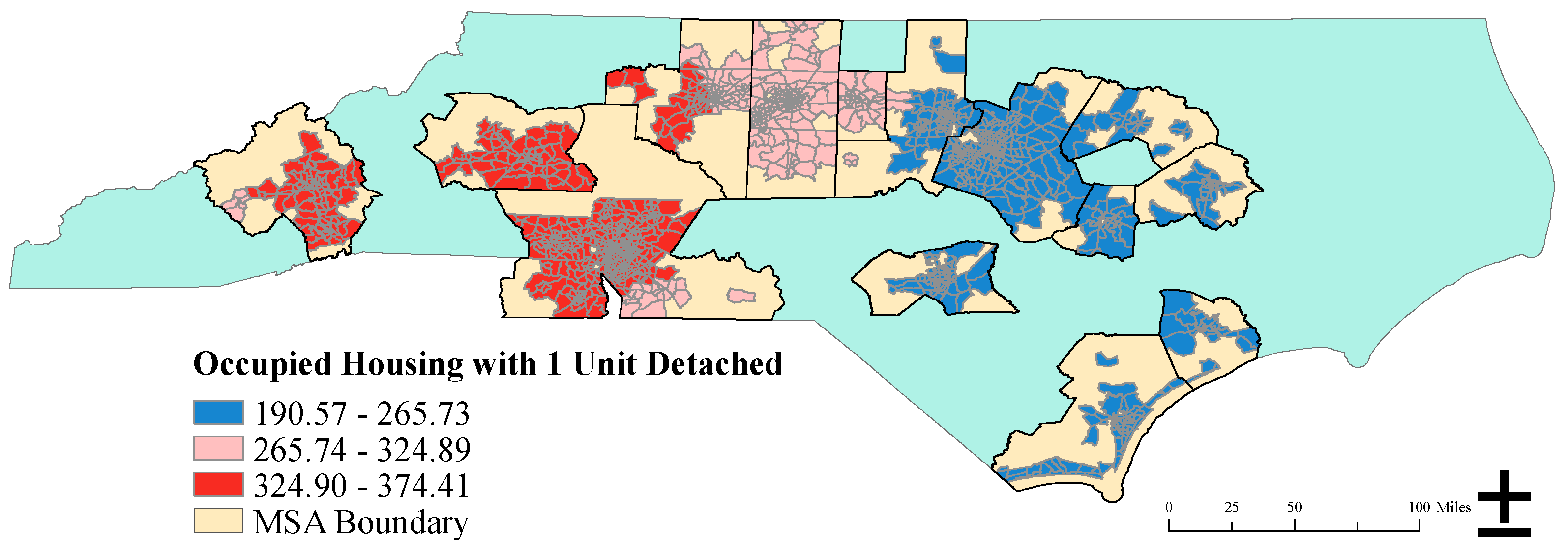
With an increase in householder median age, transportation expenditures increase in a larger amount ($40.73–$43.54) in Winston–Salem, Greensboro–High Point, Burlington, and east of Charlotte–Gastonia–Rock Hill MSAs (Figure 9). Householder median age has a lower positive influence on utility expenditures compared to transportation expenditures. However, its increase will result in households spending more on utility in the east part of study area (Figure 10a). While the lowest impacts of householder median age on utility are observed in Charlotte–Gastonia–Rock Hill, Hickory–Lenoir–Morganton, and Asheville MSAs, the results are not statistically significant (Figure 10b). The impact of percentage of housing with one unit detached on utility expenditures also varies spatially with the highest influence observed in Winston–Salem, Hickory–Lenoir–Morganton, and Charlotte–Gastonia–Rock Hill, and Asheville MSAs. With every percent increase of housings with one unit detached in these MSAs, average HH utility expenditures increase from $324.90 to $347.41 (Figure 11).
5. Discussion
Various factors have been examined in the literature to understand energy consumption using different regression analyses [44,91]. We used geographically weighted regression (GWR) method to study spatial heterogeneity in energy expenditures of households in NC. In global models, non-complete dataset with missing information might result in spatial heterogeneity [92]. Since complete datasets are difficult to obtain in many studies, applying local models to include spatial information can significantly improve the prediction results [90]. However, the problem of multicollinearity should be taken into consideration when interpreting the results. Although the explanatory variables are not collinear in this study, it should be noted that the lack of this problem in the global model does not guarantee coefficient independency in the GWR model [93].
Socioeconomic and demographic characteristics of households, urban form, housing characteristics, and local temperature are used to understand the complexity of energy consumption. As expected, OLS models show that higher income households spend more on both transportation and utilities, as richer households are interested to purchase larger houses, more goods and services, luxurious vehicles, comfortable indoor environments and recreational activities, which all result in higher energy consumption [69]. Higher education is associated with higher transportation expenditures that might be due to higher income, higher car ownership, and longer drive for commuting purpose [36,41]. Sprawl and distance from the primary city center are significant factors influencing transportation expenditures in the OLS model. This is in line with the literature suggesting the positive impact of compact development on reducing transportation consumption through transportation choice (public vs. private), automobile dependency, and vehicle miles travel (VMT) [48,52,94,95,96]. Contrary to expectations, the urban form variables were not significant predictors of HH utility expenditures in NC. Although none of the urban form factors are significant, the negative sign of sprawl indicates the lower utility expenditures spent by households living in compact areas. Housing age is also not a statistically significant factor related to utility expenditures. However, the positive correlation between housing age and energy expenditures, showing that new houses consume more energy, is in contrast with previous findings [34,97]. These results might be due to the larger size of new houses that are usually located in the less compact census tracts outside the city center.
Furthermore, the percent of detached housing has a positive impact on HH utility expenditures as it has been found in the past studies [9,53,54,55]. In addition to loosing or gaining heat in a detached home for more exposed walls, higher income households are also more likely to live in detached houses with large spaces and more rooms, all of which may suggest their higher utility consumption [9]. Higher percentage of detached housings in our study area are located outside the city center and in the areas that are representative of less compact urban forms. However, the measurement of urban form, in our case sprawl index, has remained a challenging issue for studying utility consumption. The attributes such as accessibility to green spaces, shading effects from the trees, and water bodies that may affect utility consumption [14,17] are not considered in this index. Additionally, the benefits of density on utility or transportation expenditures can be superseded by other factors such as lifestyle choices of individuals [50,95,98].
The GWR models in this research have a slightly better performance than the OLS models and provide local variations in relationships between our explanatory variables and HH energy expenditures. HH median income, householder median age, sprawl index, and distance from the primary city center explain spatial variability of HH transportation expenditures. HH median income, householder median age, and percent of housing with one unit detached are the main factors in the GWR model of utility expenditures. While the OLS results show a global trend of the impact of explanatory variables on energy expenditures, the GWR model indicates the spatial variation of the influence. For example, the OLS model shows that a census tract would have higher transportation expenditures if it is either far away from the city center or in more sprawl areas. The GWR results show where the influence of sprawl and distance from city center are higher in specific MSAs and census tracts. Identifying these local variations can be the most effective way of suggesting to urban planners where to allocate future land uses and changes in urban form to minimize HH transportation expenditures. Urban planners and policy makers can also target housing stock to reduce residential energy consumption with a transition from detached housing to attached or multifamily housing [16]. The reduction in energy consumption would be higher in the areas where GWR shows a greater relationship between housing type and HH utility expenditures illustrating by larger local coefficients. The GWR model can also offer an opportunity to see if the insignificant global parameters will show locally significant influence [84] though this was not the case for our analysis.
Both OLS and GWR modeling for HH transportation expenditures have a better fit compared to the utility model suggesting additional data requirements for the future analysis. The influence of non-economic factors such as information, attention, individual attitudes, social norms, and lifestyle on HH energy expenditures has been identified in different countries [10,99,100,101]. These variables are not included in our models because these types of data are not publicly available and are needed to be collected. The homogenous nature of NC might be the other reason that the GWR models did not provide strong results. A big advantage of the semiparametric GWR model is that it does not assume the spatial non-stationarity for all variables and allows for both global and local variables to be included in the model. However, GWR results cannot easily be transferred to other places. This is a disadvantage of GWR compared to OLS model that can be applied in similar physical settings [82]. Our aim here, however, was to capture the spatial variation of energy consumption in NC and location-specific impacts of contributing factors. The GWR model, therefore, can be a useful tool for urban planners and decision makers to develop local plans and policies to reduce and manage HH energy consumption. Socioeconomic–demographic, housing and urban form characteristics do not generally change in a short period of time and are easily available through different data sources in the U.S., thus providing adequate information for local decision makers to implement the GWR approach for other areas. Though the results may vary in different locations, the GWR modeling has been proved to be an effective method in past studies and our research for prioritizing the suitable strategies. The GWR model can be improved and extended into an optimization-modeling framework [84] that would help to solve spatial–social problems related to energy consumption. The outputs of the GWR model could serve as inputs to the optimization model [84]. For instance, an optimization model could be developed to allocate future land-use and buildings in a way to minimize energy consumption.
From a policy perspective, the general assumptions that certain policies are applicable in all parts of a country or a state need to be revisited. The results of this study show that the effects of socioeconomics and demographics, urban form, and housing characteristics on household energy consumption are different across the region. This suggests the importance of developing location-specific guidelines for decision makers in order to evaluate the consumption patterns in local areas and prioritize the suitable strategies for different areas. In addition, much focus in the U.S. has been targeted on the housing stock for improving energy efficiency of buildings through technologies. The results of this study, however, show the significant impact of socioeconomic and demographic factors and housing type on electricity and gas consumption that need to be addressed in the future policies. Local policies also need to address more compact developments in their approach to reduce transport-related energy consumption.
6. Conclusions
A spatial analytical approach was developed to study HH energy consumption in 14 MSAs of NC using geographically weighted regression (GWR) modeling at census tract geography. The estimations of the OLS and GWR models were presented to investigate the global and local effects of various explanatory factors on HH transportation and utility expenditures. The findings reveal the spatial variation of the relationship between energy expenditures and the influencing factors. To the best of our knowledge, this research is the first to have applied the GWR modeling in HH energy expenditures at census tract level in the U.S. Although there are no changes in the signs of the regression coefficients in both the OLS and the semiparametric GWR models, the explanatory power of the GWR had a slight increase characterized by higher adjusted R2, reduction of AICc, and smaller residual values.
The main contribution of this research is evaluating the influence of a range of factors in HH energy expenditures at census tract level using a spatial approach. For designing intervention aimed at changing the future land use plans for the cities across the world, the micro scale analysis is crucial. The global energy demand has raised many concerns across the world particularly for the U.S. that has the highest demand among countries [1]. A complete assessment of households’ energy consumption and its relationships to spatial urban structure need to be provided to help engineers and planners in their approach toward sustainability. The major limitation in this research is difficulty in collecting individual data that might be one of the reasons our models did not have a strong explanatory power particularly for the utility expenditures. Similarly, sprawl index does not have additional attributes (e.g., green area and tree shading) of urban form. Our housing characteristics data also have limitations such as missing information on housing shape, materials being used and ratio of window–wall. There is no complete set of data that represent such housing characteristics in census tract geography. Impact of individuals’ attitude and life style choice on energy consumption should be evaluated through detailed HH surveys. Although obtaining such data for a state such as NC is practically impossible, it should be noted that technology or planning alone might not encourage people to decrease their consumptions. Another limitation is the homogenous nature of NC. Applying our GWR model to other states might provide stronger and more reliable results. Developing policies to address these issues, improving the goodness of fit of GWR model, and extending the model to optimization frameworks remain some areas for future research.
Author Contributions
S.S. originally came up with the idea and designed the conceptual framework of the research with N.P. and H.K.; N.P. primarily collected and analyzed the data and wrote the original draft; H.K. contributed to the data acquisition and analysis; S.S. provided advices on results and modified the manuscript.
Acknowledgments
The authors acknowledge financial support from the University of North Carolina at Greensboro. We are thankful to Dominique Haller, an undergraduate research assistant, for doing some preliminary data analysis. We also wish to thank three anonymous reviewers for their valuable feedback that improved this paper. All shortcomings are nonetheless ours.
Conflicts of Interest
The authors declare no conflict of interest.
References
- Salari, M.; Javid, R.J. Residential energy demand in the United States: Analysis using static and dynamic approaches. Energy Policy 2016, 98, 637–649. [Google Scholar] [CrossRef]
- U.S. Energy Information Administration. International Energy Outlook 2017. Available online: https://www.eia.gov/outlooks/ieo/ (accessed on 24 March 2018).
- Jones, C.; Kammen, D.M. Spatial Distribution of U.S. Household Carbon Footprints Reveals Suburbanization Undermines Greenhouse Gas Benefits of Urban Population Density. Environ. Sci. Technol. 2014, 48, 895–902. [Google Scholar] [CrossRef] [PubMed]
- Liu, L.C.; Wu, G.; Wang, J.N.; Wei, Y.M. China’s carbon emissions from urban and rural households during 1992–2007. J. Clean. Prod. 2011, 19, 1754–1762. [Google Scholar] [CrossRef]
- U.S. Environmental Protection Agency. DRAFT Inventory of U.S. Greenhouse Gas Emissions and Sinks: 1990–2016. Available online: https://www.epa.gov/ghgemissions/draft-inventory-us-greenhouse-gas-emissions-and-sinks-1990-2016 (accessed on 24 March 2018).
- Raftery, A.E.; Zimmer, A.; Frierson, D.M.W.; Startz, R.; Liu, P. Less than 2 °C warming by 2100 unlikely. Nat. Clim. Chang. 2017, 7, 637–641. [Google Scholar] [CrossRef]
- Kopp, R.E.; Kemp, A.C.; Bittermann, K.; Horton, B.P.; Donnelly, J.P.; Gehrels, W.R.; Hay, C.C.; Mitrovica, J.X.; Morrow, E.D.; Rahmstorf, S. Temperature-driven global sea-level variability in the Common Era. Proc. Natl. Acad. Sci. USA 2016, 113, E1434–E1441. [Google Scholar] [CrossRef] [PubMed]
- Hsiang, S.; Kopp, R.; Jina, A.; Rising, J.; Delgado, M.; Mohan, S.; Rasmussen, D.J.; Muir-Wood, R.; Wilson, P.; Oppenheimer, M.; et al. Estimating economic damage from climate change in the United States. Science 2017, 356, 1362–1369. [Google Scholar] [CrossRef] [PubMed]
- Estiri, H. Household Energy Consumption and Housing Choice in the U.S. Residential Sector. Hous. Policy Debate 2016, 26, 231–250. [Google Scholar] [CrossRef]
- Chitnis, M.; Hunt, L.C. What drives the change in UK household energy expenditure and associated CO2 emissions? Implication and forecast to 2020. Appl. Energy 2012, 94, 202–214. [Google Scholar] [CrossRef]
- Lévy, J.-P.; Belaïd, F. The determinants of domestic energy consumption in France: Energy modes, habitat, households and life cycles. Renew. Sustain. Energy Rev. 2018, 81, 2104–2114. [Google Scholar] [CrossRef]
- Van den Brom, P.; Meijer, A.; Visscher, H. Performance gaps in energy consumption: Household groups and building characteristics. Build. Res. Inf. 2018, 46, 54–70. [Google Scholar] [CrossRef]
- Véliz, K.D.; Kaufmann, R.K.; Cleveland, C.J.; Stoner, A.M.K. The effect of climate change on electricity expenditures in Massachusetts. Energy Policy 2017, 106, 1–11. [Google Scholar] [CrossRef]
- Ye, H.; He, X.; Song, Y.; Li, X.; Zhang, G.; Lin, T.; Xiao, L. A sustainable urban form: The challenges of compactness from the viewpoint of energy consumption and carbon emission. Energy Build. 2015, 93, 90–98. [Google Scholar] [CrossRef]
- Shammin, M.R.; Herendeen, R.A.; Hanson, M.J.; Wilson, E.J.H. A multivariate analysis of the energy intensity of sprawl versus compact living in the U.S. for 2003. Ecol. Econ. 2010, 69, 2363–2373. [Google Scholar] [CrossRef]
- Ewing, R.; Rong, F. The impact of urban form on U.S. residential energy use. Hous. Policy Debate 2008, 19, 1–30. [Google Scholar] [CrossRef]
- Silva, M.; Oliveira, V.; Leal, V. Urban Form and Energy Demand. J. Plan. Lit. 2017, 32, 346–365. [Google Scholar] [CrossRef]
- Wang, M.; Madden, M.; Liu, X. Exploring the Relationship between Urban Forms and CO2 Emissions in 104 Chinese Cities. J. Urban Plan. Dev. 2017, 143, 4017014. [Google Scholar] [CrossRef]
- Parshall, L.; Gurney, K.; Hammer, S.A.; Mendoza, D.; Zhou, Y.; Geethakumar, S. Modeling energy consumption and CO2 emissions at the urban scale: Methodological challenges and insights from the United States. Energy Policy 2010, 38, 4765–4782. [Google Scholar] [CrossRef]
- Faller, F. A practice approach to study the spatial dimensions of the energy transition. Environ. Innov. Soc. Transit. 2016, 19, 85–95. [Google Scholar] [CrossRef]
- Stoeglehner, G.; Niemetz, N.; Kettl, K.-H. Spatial dimensions of sustainable energy systems: New visions for integrated spatial and energy planning. Energy Sustain. Soc. 2011, 1, 2. [Google Scholar] [CrossRef]
- Heath, G.W.; Brownson, R.C.; Kruger, J.; Miles, R.; Powell, K.E.; Ramsey, L.T. The Effectiveness of Urban Design and Land Use and Transport Policies and Practices to Increase Physical Activity: A Systematic Review. J. Phys. Act. Health 2006, 3, S55–S76. [Google Scholar] [CrossRef] [PubMed]
- Guo, W.; Zhao, T.; Dai, H. Calculation and decomposition of regional household energy consumption in China: Based on perspectives of urbanization and residents’ consumption. Chin. J. Popul. Resour. Environ. 2017, 15, 132–141. [Google Scholar] [CrossRef]
- Ding, Y.; Qu, W.; Niu, S.; Liang, M.; Qiang, W.; Hong, Z. Factors Influencing the Spatial Difference in Household Energy Consumption in China. Sustainability 2016, 8, 1285. [Google Scholar] [CrossRef]
- Nelson, J.K.; Brewer, C.A. Evaluating data stability in aggregation structures across spatial scales: Revisiting the modifiable areal unit problem. Cartogr. Geogr. Inf. Sci. 2017, 44, 35–50. [Google Scholar] [CrossRef]
- Weir-Smith, G. Changing boundaries: Overcoming modifiable areal unit problems related to unemployment data in South Africa. S. Afr. J. Sci. 2016, 112. [Google Scholar] [CrossRef]
- Valenzuela, C.; Valencia, A.; White, S.; Jordan, J.A.; Cano, S.; Keating, J.; Nagorski, J.; Potter, L.B. An analysis of monthly household energy consumption among single-family residences in Texas, 2010. Energy Policy 2014, 69, 263–272. [Google Scholar] [CrossRef]
- Tian, W.; Song, J.; Li, Z. Spatial regression analysis of domestic energy in urban areas. Energy 2014, 76, 629–640. [Google Scholar] [CrossRef]
- Tobler, W.R. A Computer Movie Simulating Urban Growth in the Detroit Region. Econ. Geogr. 1970, 46, 234–240. [Google Scholar] [CrossRef]
- Wu, R.; Zhang, J.; Bao, Y.; Tong, S. Using a Geographically Weighted Regression Model to Explore the Influencing Factors of CO2 Emissions from Energy Consumption in the Industrial Sector. Pol. J. Environ. Stud. 2016, 25, 2641–2651. [Google Scholar] [CrossRef]
- Brunsdon, C.; Fotheringham, S.; Charlton, M. Geographically Weighted Regression. J. R. Stat. Soc. Ser. D 1998, 47, 431–443. [Google Scholar] [CrossRef]
- Oshan, T.M.; Fotheringham, A.S. A Comparison of Spatially Varying Regression Coefficient Estimates Using Geographically Weighted and Spatial-Filter-Based Techniques. Geogr. Anal. 2018, 50, 53–75. [Google Scholar] [CrossRef]
- Institute for Energy Research. North Carolina: An Energy and Economic Analysis; Institute for Energy Research: Washington, DC, USA. Available online: https://instituteforenergyresearch.org/analysis/north-carolina-an-energy-and-economic-analysis/ (accessed on 24 March 2018).
- Salari, M.; Javid, R.J. Modeling household energy expenditure in the United States. Renew. Sustain. Energy Rev. 2017, 69, 822–832. [Google Scholar] [CrossRef]
- Gatersleben, B.; Steg, L.; Vlek, C. Measurement and Determinants of Environmentally Significant Consumer Behavior. Environ. Behav. 2002, 34, 335–362. [Google Scholar] [CrossRef]
- Hasan, S.A.; Mozumder, P. Income and energy use in Bangladesh: A household level analysis. Energy Econ. 2017, 65, 115–126. [Google Scholar] [CrossRef]
- Han, S.S.; Karuppannan, S. Non-transport household energy consumption in Adelaide and Melbourne. Local Environ. 2016, 21, 290–309. [Google Scholar] [CrossRef]
- Wei, T.; Zhu, Q.; Glomsrød, S. Energy spending and household characteristics of floating population: Evidence from Shanghai. Energy Sustain. Dev. 2014, 23, 141–149. [Google Scholar] [CrossRef]
- Druckman, A.; Jackson, T. Household energy consumption in the UK: A highly geographically and socio-economically disaggregated model. Energy Policy 2008, 36, 3167–3182. [Google Scholar] [CrossRef] [Green Version]
- Pothitou, M.; Hanna, R.F.; Chalvatzis, K.J. Environmental knowledge, pro-environmental behaviour and energy savings in households: An empirical study. Appl. Energy 2016, 184, 1217–1229. [Google Scholar] [CrossRef]
- Ding, C.; Liu, C.; Zhang, Y.; Yang, J.; Wang, Y. Investigating the impacts of built environment on vehicle miles traveled and energy consumption: Differences between commuting and non-commuting trips. Cities 2017, 68, 25–36. [Google Scholar] [CrossRef]
- Miah, M.D.; Kabir, R.R.M.S.; Koike, M.; Akther, S.; Yong Shin, M. Rural household energy consumption pattern in the disregarded villages of Bangladesh. Energy Policy 2010, 38, 997–1003. [Google Scholar] [CrossRef]
- Yohanis, Y.G. Domestic energy use and householders’ energy behaviour. Energy Policy 2012, 41, 654–665. [Google Scholar] [CrossRef]
- Chen, J.; Wang, X.; Steemers, K. A statistical analysis of a residential energy consumption survey study in Hangzhou, China. Energy Build. 2013, 66, 193–202. [Google Scholar] [CrossRef]
- Brounen, D.; Kok, N.; Quigley, J.M. Residential energy use and conservation: Economics and demographics. Eur. Econ. Rev. 2012, 56, 931–945. [Google Scholar] [CrossRef]
- Cashin, D.; McGranahan, L. Household Energy Expenditures, 1982–2005. Federal Reserve Bank of Chicago: Chicago, IL, USA. Available online: https://www.chicagofed.org/publications/chicago-fed-letter/2006/june-227 (accessed on 9 May 2018).
- Dillon, H.S.; Saphores, J.D.; Boarnet, M.G. The impact of urban form and gasoline prices on vehicle usage: Evidence from the 2009 National Household Travel Survey. Res. Transp. Econ. 2015, 52, 23–33. [Google Scholar] [CrossRef]
- Glaeser, E.L.; Kahn, M.E. The greenness of cities: Carbon dioxide emissions and urban development. J. Urban Econ. 2010, 67, 404–418. [Google Scholar] [CrossRef]
- Baur, A.H.; Förster, M.; Kleinschmit, B. The spatial dimension of urban greenhouse gas emissions: Analyzing the influence of spatial structures and LULC patterns in European cities. Landsc. Ecol. 2015, 30, 1195–1205. [Google Scholar] [CrossRef]
- Heinonen, J.; Junnila, S. Case study on the carbon consumption of two metropolitan cities. Int. J. Life Cycle Assess. 2011, 16, 569–579. [Google Scholar] [CrossRef]
- Dai, H.; Masui, T.; Matsuoka, Y.; Fujimori, S. The impacts of China’s household consumption expenditure patterns on energy demand and carbon emissions towards 2050. Energy Policy 2012, 50, 736–750. [Google Scholar] [CrossRef]
- Holden, E.; Norland, I.T. Three challenges for the compact city as a sustainable urban form: Household consumption of energy and transport in eight residential areas in the Greater. Urban Stud. 2005, 42, 2145–2166. [Google Scholar] [CrossRef]
- Longhi, S. Residential energy expenditures and the relevance of changes in household circumstances. Energy Econ. 2015, 49, 440–450. [Google Scholar] [CrossRef]
- Curtis, J.; Pentecost, A. Household fuel expenditure and residential building energy efficiency ratings in Ireland. Energy Policy 2015, 76, 57–65. [Google Scholar] [CrossRef]
- Tso, G.K.F.; Guan, J. A multilevel regression approach to understand effects of environment indicators and household features on residential energy consumption. Energy 2014, 66, 722–731. [Google Scholar] [CrossRef]
- Zakaria, R.; Amirazar, A.; Mustaffar, M.; Mohammad Zin, R.; Abd Majid, M.Z. Daylight Factor for Energy Saving in Retrofitting Institutional Building. Adv. Mater. Res. 2013, 724–725, 1630–1635. [Google Scholar] [CrossRef]
- U.S. Energy Information Administration. 2015 Residential Energy Consumption Survey (RECS). Available online: https://www.eia.gov/consumption/residential/ (accessed on 24 March 2018).
- Sultana, S.; Weber, J. The Nature of Urban Growth and the Commuting Transition: Endless Sprawl or a Growth Wave? Urban Stud. 2014, 51, 544–576. [Google Scholar] [CrossRef]
- Ewing, R.; Cervero, R. Travel and the built environment. J. Am. Plan. Assoc. 2010, 76, 265–294. [Google Scholar] [CrossRef]
- Haas, P.; Morse, S.; Becker, S.; Young, L.; Esling, P. The influence of spatial and household characteristics on household transportation costs. Res. Transp. Bus. Manag. 2013, 7, 14–26. [Google Scholar] [CrossRef]
- Wang, X.; Liu, C.; Kostyniuk, L.; Shen, Q.; Bao, S. The influence of street environments on fuel efficiency: Insights from naturalistic driving. Int. J. Environ. Sci. Technol. 2014, 11, 2291–2306. [Google Scholar] [CrossRef]
- Brownstone, D.; Golob, T.F. The impact of residential density on vehicle usage and energy consumption. J. Urban Econ. 2009, 65, 91–98. [Google Scholar] [CrossRef]
- Susilo, Y.; Stead, D. Individual Carbon Dioxide Emissions and Potential for Reduction in the Netherlands and the United Kingdom. Transp. Res. Rec. J. Transp. Res. Board 2009, 2139, 142–152. [Google Scholar] [CrossRef]
- Sultana, S.; Salon, D.; Kuby, M. Transportation sustainability in the urban context: A comprehensive review. Urban Geogr. 2017, 1–30. [Google Scholar] [CrossRef]
- Bessec, M.; Fouquau, J. The non-linear link between electricity consumption and temperature in Europe: A threshold panel approach. Energy Econ. 2008, 30, 2705–2721. [Google Scholar] [CrossRef]
- Franco, G.; Sanstad, A.H. Climate change and electricity demand in California. Clim. Chang. 2007, 87, 139–151. [Google Scholar] [CrossRef]
- Hekkenberg, M.; Moll, H.C.; Uiterkamp, A.J.M.S. Dynamic temperature dependence patterns in future energy demand models in the context of climate change. Energy 2009, 34, 1797–1806. [Google Scholar] [CrossRef]
- Zhou, Y.; Clarke, L.; Eom, J.; Kyle, P.; Patel, P.; Kim, S.H.; Dirks, J.; Jensen, E.; Liu, Y.; Rice, J.; et al. Modeling the effect of climate change on U.S. state-level buildings energy demands in an integrated assessment framework. Appl. Energy 2014, 113, 1077–1088. [Google Scholar] [CrossRef]
- Zhang, X.; Luo, L.; Skitmore, M. Household carbon emission research: An analytical review of measurement, influencing factors and mitigation prospects. J. Clean. Prod. 2015, 103, 873–883. [Google Scholar] [CrossRef] [Green Version]
- U.S. Energy Information Administration. 2015 State Energy Data System (SEDS). Available online: https://www.eia.gov/state/?sid=NC#tabs-2 (accessed on 24 March 2018).
- U.S. Energy Information Administration. North Carolina State Energy Profile. Available online: https://www.eia.gov/state/?sid=NC (accessed on 24 March 2018).
- United States Census Bureau. Census Bureau Reports. Available online: https://www.census.gov/newsroom/press-releases/2017/estimates-idaho.html (accessed on 24 March 2018).
- SymplyAnalytics. Available online: https://simplyanalytics.com/ (accessed on 24 March 2018).
- United States census Bureau. American Community Survey. Available online: https://factfinder.census.gov/faces/nav/jsf/pages/index.xhtml (accessed on 24 March 2018).
- Ewing, R.; Hamidi, S. Measuring Urban Sprawl and Validating Sprawl Measures. Available online: https://gis.cancer.gov/tools/urban-sprawl/ (accessed on 24 March 2018).
- Van Wee, B.; Handy, S. Key research themes on urban space, scale, and sustainable urban mobility. Int. J. Sustain. Transp. 2016, 10, 18–24. [Google Scholar] [CrossRef]
- North Carolina Department of Transportation. GIS Data Layers, Road Data. Available online: https://connect.ncdot.gov/resources/gis/pages/gis-data-layers.aspx (accessed on 24 March 2018).
- South Carolina Department of Transportation. GIS/Mapping. Available online: http://info2.scdot.org/sites/GIS/SitePages/default.aspx# (accessed on 24 March 2018).
- Berrigan, D.; Troiano, R.P. The association between urban form and physical activity in U.S. adults. Am. J. Prev. Med. 2002, 23, 74–79. [Google Scholar] [CrossRef]
- Voulgaris, C.T.; Taylor, B.D.; Blumenberg, E.; Brown, A.; Ralph, K. Synergistic neighborhood relationships with travel behavior: An analysis of travel in 30,000 US neighborhoods. J. Transp. Land Use 2016, 10, 437–461. [Google Scholar] [CrossRef]
- National Centers for Environmental Information. Land-Based Station Data. Available online: https://www.ncdc.noaa.gov/data-access/land-based-station-data (accessed on 24 March 2018).
- Ivajnšič, D.; Kaligarič, M.; Žiberna, I. Geographically weighted regression of the urban heat island of a small city. Appl. Geogr. 2014, 53, 341–353. [Google Scholar] [CrossRef]
- Nakaya, T. GWR4.09 User Manual. Available online: http://gwr.maynoothuniversity.ie/gwr4-software/ (accessed on 24 March 2018).
- Wang, C.; Chen, N. A geographically weighted regression approach to investigating the spatially varied built-environment effects on community opportunity. J. Transp. Geogr. 2017, 62, 136–147. [Google Scholar] [CrossRef]
- Slagle, M. A Comparison of Spatial Statistical Methods in a School Finance Policy Context. J. Educ. Financ. 2010, 35, 199–216. [Google Scholar] [CrossRef]
- Brunsdon, C.; Fotheringham, A.S.; Charlton, M. Some Notes on Parametric Significance Tests for Geographically Weighted Regression. J. Reg. Sci. 1999, 39, 497–524. [Google Scholar] [CrossRef]
- Chiou, Y.-C.; Jou, R.-C.; Yang, C.-H. Factors affecting public transportation usage rate: Geographically weighted regression. Transp. Res. Part A Policy Pract. 2015, 78, 161–177. [Google Scholar] [CrossRef]
- U.S. Bureau of Labor Statistics. TED: The Economics Daily. Available online: https://www.bls.gov/opub/ted/2016/household-spending-increased-4-point-6-percent-from-2014-to-2015.htm (accessed on 24 March 2018).
- U.S. Department of Transportation. Transportation Economic Trends. Available online: https://www.bts.gov/content/transportation-economic-trends (accessed on 24 March 2018).
- Ciotoli, G.; Voltaggio, M.; Tuccimei, P.; Soligo, M.; Pasculli, A.; Beaubien, S.E.; Bigi, S. Geographically weighted regression and geostatistical techniques to construct the geogenic radon potential map of the Lazio region: A methodological proposal for the European Atlas of Natural Radiation. J. Environ. Radioact. 2017, 166, 355–375. [Google Scholar] [CrossRef] [PubMed]
- Min, J.; Hausfather, Z.; Lin, Q.F. A high-resolution statistical model of residential energy end use characteristics for the United States. J. Ind. Ecol. 2010, 14, 791–807. [Google Scholar] [CrossRef]
- Fotheringham, A.S.; Charlton, M.; Brunsdon, C. Two techniques for exploring non-stationarity in geographical data. Geogr. Syst. 1997, 4, 59–82. [Google Scholar]
- Wheeler, D.; Tiefelsdorf, M. Multicollinearity and correlation among local regression coefficients in geographically weighted regression. J. Geogr. Syst. 2005, 7, 161–187. [Google Scholar] [CrossRef]
- Delmelle, E.; Zhou, Y.; Thill, J.-C. Densification without Growth Management? Evidence from Local Land Development and Housing Trends in Charlotte, North Carolina, USA. Sustainability 2014, 6, 3975–3990. [Google Scholar] [CrossRef]
- Muratori, M.; Moran, M.J.; Serra, E.; Rizzoni, G. Highly-resolved modeling of personal transportation energy consumption in the United States. Energy 2013, 58, 168–177. [Google Scholar] [CrossRef]
- Jensen, J.O.; Christensen, T.H.; Gram-hanssen, K. Sustainable urban development—Compact cities or consumer practices? Dan. J. Geoinform. Land Manag. 2011, 46, 1–14. [Google Scholar]
- Droutsa, K.G.; Kontoyiannidis, S.; Dascalaki, E.G.; Balaras, C.A. Ranking cost effective energy conservation measures for heating in Hellenic residential buildings. Energy Build. 2014, 70, 318–332. [Google Scholar] [CrossRef]
- Ala-Mantila, S.; Heinonen, J.; Junnila, S. Relationship between urbanization, direct and indirect greenhouse gas emissions, and expenditures: A multivariate analysis. Ecol. Econ. 2014, 104, 129–139. [Google Scholar] [CrossRef]
- Chitnis, M.; Druckman, A.; Hunt, L.C.; Jackson, T.; Milne, S. Forecasting scenarios for UK household expenditure and associated GHG emissions: Outlook to 2030. Ecol. Econ. 2012, 84, 129–141. [Google Scholar] [CrossRef] [Green Version]
- Allcott, H. Social norms and energy conservation. J. Public Econ. 2011, 95, 1082–1095. [Google Scholar] [CrossRef]
- Weber, C.; Perrels, A. Modelling lifestyle effects on energy demand and related emissions. Energy Policy 2000, 28, 549–566. [Google Scholar] [CrossRef]
Figure 1.
Theoretical framework for household energy expenditures.

Figure 2.
Study area. MSA: Metropolitan statistical area.

Figure 3.
Methodological process. ANOVA: analysis of variance; OLS: ordinary least squares; GWR: geographically weighted regression.
Figure 3.
Methodological process. ANOVA: analysis of variance; OLS: ordinary least squares; GWR: geographically weighted regression.

Figure 4.
Average household expenditures (in $) in 14 MSAs of North Carolina.

Figure 5.
Hot and cold spots of transportation (a) and utility (b) expenditures.

Figure 6.
Geographical variability of local R2 for transportation (a) and utility (b) models.

Figure 7.
Local coefficients of sprawl (a) and distance from city center (b) with its corresponding local t-values (c) for transportation model.
Figure 7.
Local coefficients of sprawl (a) and distance from city center (b) with its corresponding local t-values (c) for transportation model.

Figure 8.
Local coefficients of household median income for transportation (a) and utility (b) models.
Figure 8.
Local coefficients of household median income for transportation (a) and utility (b) models.

Figure 9.
Local coefficients of household median age for transportation model.

Figure 10.
Local coefficients of household median age utility model (a) with the corresponding local t-values (b).
Figure 10.
Local coefficients of household median age utility model (a) with the corresponding local t-values (b).

Figure 11.
Local coefficients of percent of occupied housing with one unit detached for utility model.
Figure 11.
Local coefficients of percent of occupied housing with one unit detached for utility model.


Table 1.
The four factors and their main explanatory variables.
| Factor | Variable |
|---|---|
| Socioeconomics and demographics |
|
| Urban form |
|
| Housing characteristics |
|
| Temperature |
|
Table 2.
Ordinary least squares (OLS) results for transportation model.
| Multiple R-Squared | 0.42 | Adjusted R-Squared | 0.41 |
| Akaike Information Criterion (AICc) | 24,971.48 | ||
| Joint F-Statistic | 141 | Probability | 0.000000 ** |
| Joint Wald Statistic | 784.99 | Probability | 0.000000 ** |
| Koenker (BP) Statistic | 113.43 | Probability | 0.000000 ** |
| Jarque–Bera Statistic | 34.52 | Probability | 0.000000 ** |
| Moran Index | 0.005 | Probability | 0.04 * |
| Variable 1 | Coefficient | p-Value | VIF |
| Household median income | 0.03 | 0.000000 * | 4.62 |
| Education_bachelor | 2847.93 | 0.001985 * | 4.63 |
| Education_less than high school | −2389.26 | 0.006947 * | 2.76 |
| Householder median age | 37.68 | 0.000067 * | 1.42 |
| Sprawl | −16.10 | 0.000001 * | 1.67 |
| Distance from city center | 23.15 | 0.000800 * | 1.37 |
1 Only Significant variables are reported. ** Statistically significant p value (p < 0.01); * Statistically significant p value (p < 0.05).
Table 3.
OLS results for utility model.
| Multiple R-Squared | 0.13 | Adjusted R-Squared | 0.12 |
| Akaike Information Criterion (AICc) | 20,490.24 | ||
| Joint F-Statistic | 17.18 | Probability | 0.000000 ** |
| Joint Wald Statistic | 176.68 | Probability | 0.000000 ** |
| Koenker (BP) Statistic | 52.20 | Probability | 0.000001 ** |
| Jarque–Bera Statistic | 38.31 | Probability | 0.000000 ** |
| Moran Index | 0.0002 | Probability | 0.8 |
| Variable 1 | Coefficient | p-Value | VIF |
| Household median income | 0.003 | 0.000760 * | 6.26 |
| Householder median age | 6.31 | 0.007251 * | 2.23 |
| Percent of occupied housings with one unit detached | 232.52 | 0.002995 * | 2.63 |
1 Only significant variables are reported. ** Statistically significant p value (p < 0.01); * Statistically significant p value (p < 0.05).
Table 4.
Summary of results from the semiparametric GWR model analysis.
| Transportation Model | Utility Model | |
|---|---|---|
| Bandwidth | 624 | 767 |
| Maximum likelihood (ML) based sigma estimate | 1855.70 | 370.40 |
| Unbiased sigma estimate | 1864.77 | 373.12 |
| AICc | 24,966.14 | 20,484.03 |
| R square | 0.42 | 0.14 |
| Adjusted R square | 0.42 | 0.13 |
| Residual sum of squares | 4,800,456,560 | 191,249,118 |
Table 5.
Geographical variability tests of significant local coefficients.
| Transportation | |||
| Variable | F-Value | DIFF of Criterion | t-Value |
| Household median income | 17.06 | −9.87 | 9.04 |
| Householder median age | 6.38 | −3.44 | 4.03 |
| Sprawl | 4.96 | −2.39 | −5.13 |
| Distance from city center | 4.98 | −2.50 | 3.37 |
| Utility | |||
| Variable | F-Value | DIFF of Criterion | t-Value |
| Household median income | 13.09 | −5.13 | 3.39 |
| Householder median age | 6.00 | −2.36 | 2.69 |
| Percent of occupied housings with one unit detached | 4.73 | −1.51 | 2.97 |
Table 6.
Summary statistics for statistically significant varying coefficients.
| Transportation | ||||||
| Variable | Mean | Median | STD | Min | Max | Range |
| Intercept | 5746.69 | 5653.38 | 463.99 | 5140.24 | 6547.30 | 1407.06 |
| Household median income | 0.035 | 0.035 | 0.003 | 0.031 | 0.039 | 0.008 |
| Householder median age | 39.60 | 39.63 | 1.87 | 35.28 | 43.54 | 8.26 |
| Sprawl | −18.30 | −19.21 | 2.05 | −21.97 | −15.05 | 6.92 |
| Distance from city center | 20.39 | 21.76 | 3.24 | 15.17 | 24.72 | 9.54 |
| Utility | ||||||
| Variable | Mean | Median | STD | Min | Max | Range |
| Intercept | −1395.53 | −1847.77 | 1184.05 | −2952.68 | 480.68 | 3433.36 |
| Household median income | 0.0029 | 0.0032 | 0.0004 | 0.0023 | 0.0035 | 0.0012 |
| Householder median age | 4.94 | 4.41 | 1.81 | 1.92 | 7.58 | 5.67 |
| Percent of occupied housings with one unit detached | 290.69 | 310.61 | 55.46 | 190.57 | 374.41 | 183.831 |
Table 7.
GWR ANOVA results for transportation model.
| Source | Sum of Squares | Degree of Freedom | Mean Square | F-Value |
|---|---|---|---|---|
| Global Residuals | 4,851,701,377.946 | 1386 | ||
| GWR Improvement | 51,244,817.623 | 5.509 | 9,301,488.211 | |
| GWR Residuals | 4,800,456,560.323 | 1380.491 | 3,477,355.268 | 2.674874 |
Table 8.
GWR ANOVA results for utility model.
| Source | Sum of Squares | Degree of Freedom | Mean Square | F-Value |
|---|---|---|---|---|
| Global Residuals | 193,469,117.859 | 1381 | ||
| GWR Improvement | 2,219,999.078 | 7.243 | 306,484.814 | |
| GWR Residuals | 191,249,118.780 | 1373.757 | 139,216.162 | 2.201503 |
© 2018 by the authors. Licensee MDPI, Basel, Switzerland. This article is an open access article distributed under the terms and conditions of the Creative Commons Attribution (CC BY) license (http://creativecommons.org/licenses/by/4.0/).
Share and Cite
MDPI and ACS Style
Sultana, S.; Pourebrahim, N.; Kim, H. Household Energy Expenditures in North Carolina: A Geographically Weighted Regression Approach. Sustainability 2018, 10, 1511. https://0-doi-org.brum.beds.ac.uk/10.3390/su10051511
AMA Style
Sultana S, Pourebrahim N, Kim H. Household Energy Expenditures in North Carolina: A Geographically Weighted Regression Approach. Sustainability. 2018; 10(5):1511. https://0-doi-org.brum.beds.ac.uk/10.3390/su10051511
Chicago/Turabian StyleSultana, Selima, Nastaran Pourebrahim, and Hyojin Kim. 2018. "Household Energy Expenditures in North Carolina: A Geographically Weighted Regression Approach" Sustainability 10, no. 5: 1511. https://0-doi-org.brum.beds.ac.uk/10.3390/su10051511
Note that from the first issue of 2016, this journal uses article numbers instead of page numbers. See further details here.